Abstract
Submesoscale eddies play an important role in the energy transfer from the mesoscale down to the dissipative range, as well as in tracer transport. They carry inorganic matter, nutrients and biomass; in addition, they may act as pollutant conveyors. However, synoptic observations of these features need high resolution sampling, in both time and space, making their identification challenging. Therefore, HF coastal radar were and are successfully used to accurately identify, track and describe them. In this paper we tested two already existing algorithms for the automated detection of submesoscale eddies. We applied these algorithms to HF radar velocity fields measured by a network of three radar systems operating in the Gulf of Naples. Both methods showed shortcomings, due to the high non-geostrophy of the observed currents. For this reason we developed a third, novel algorithm that proved to be able to detect highly asymmetrical eddies, often not properly identified by the previous ones. We used the results of the application of this algorithm to estimate the eddy boundary profiles and the eddy spatial distribution.
1. Introduction
Transport in the ocean develops over an extremely wide range of scales, from the basin to the dissipation scale (e.g., [1]). Our ability to observe and/or to model processes at smaller and smaller scales has greatly increased over the last few decades. Phenomena that in the very recent past could not be detected or described, and thus needed to be parametrized in terms of larger scales (e.g., [2,3]), are now subjects of consolidated research, as is the case of mesoscale features. Now, our focus has shifted to smaller dynamics, such as submesoscale motions. In the wide range of turbulent processes in the ocean, submesoscale eddies are the most volatile ones, due to their short lifetime (few hours) and length scale (below 10 km).
Submesoscale eddies principally act as energy conveyors from the mesoscale to the microscale, and play a crucial ecological role: they may influence the state of health of ocean regions through their ability to carry heat, inorganic matter, nutrients and biomass ([4,5]), ensuring the connectivity between different ecosystems ([6]). They are particularly important for phytoplankton, as they develop over timescales similar to those of phytoplankton growth ([7]), moreover, they may act as carriers of pollutants (see, e.g., [8]). Consequently the detection of eddies, behind its inherent interest, is crucial also for environmental applications.
As more and more synoptic, high resolution data on mesoscale and submesoscale eddies has become available, thanks to remote sensing techniques at different resolutions, automatic eddy detection methods have gained importance and interest. In the recent past, several eddy detection algorithms ([9,10,11,12,13]) have been developed and applied to velocity fields derived from altimeter data, numerical model outputs and HF radar observations. They can be divided into three families: geometrical, dynamical and hybrid ones. The definition depends on the flow characteristics extrapolated by the algorithm itself, that can be geometrical, dynamical or both (e.g., [9,10,11] and respectively). However, the existing methods have been mainly conceived for meso and larger scale recirculations, which display different kinematic characteristics than submesoscale eddies, in particular in terms of divergence and (a)symmetry of the flow field.
Mesoscale eddies scale with the first internal Rossby radius ([14,15]), which is of the order of 10 km in the Mediterranean (5 to 12 km according to [16]) and four to ten times as large in the north Atlantic ([17]). Differently, submesoscale surface eddies have characteristic lengths starting from km up to the mesoscale ([8,18]). They are completely confined in the surface mixed layer, within depths going from tens to hundreds of meters. Therefore, since their relative Rossby and Froude numbers, and , are not small, these structures show highly non-geostrophic behavior, high divergent flow patterns and strong asymmetries. As a consequence, the aforementioned algorithms, typically designed to capture the features of vortices in geostrophic balance, may fail in detecting submesoscale eddies as they are often unable to characterize highly deformed, divergent or convergent motions. For this reason, we have designed a novel algorithm, presented in this paper, that has proved to be able to capture the noncircular symmetry and the divergent character of submesoscale recirculations.
High resolution data is needed in order to identify submesoscale motions. In this framework, HF radars are proving to be an almost irreplaceable tool: They are land-based remote sensing instruments which allow to observe surface currents at very high spatial and temporal resolution, thus suitable to monitor such small scale phenomena ([19,20]). Other remote sensing techniques are available, even with much higher spatial resolution, and are thus able to detect submesoscale flow features ([21,22,23], but they have very long revisit periods with respect to the hourly sampling provided by coastal radars, thus allowing for detecting but not for tracking such features.
In this study we have utilized HF radar observations of surface currents in the Gulf of Naples (GoN), a semi-enclosed area of the Tyrrhenian, a sub-basin of the western Mediterranean Sea. The GoN is surrounded by a coast characterized by a quite uneven orography, dominated by the presence of the Vesuvius volcano and of Mount Faito in the East, both exceeding 1000 m altitude, and of a number of lower hills very close to the northern coastline. It has a complex bathymetry, with an average depth of 170 m which reaches down to more than 800 m in correspondence of two major canyons, the Magnaghi and the Dohrn, which carve the shelf across the threshold connecting the Gulf with the open Tyrrhenian Sea. Its surface circulation is mainly wind driven, with a strong seasonal regime ([24,25]), even though the offshore circulation of the Southern Tyrrhenian may occasionally affect the current pattern in the interior of the GoN ([25] and references therein). The Gulf represents a very complex system: It hosts a heavily anthropized coastline, with industrial settlements in the immediate vicinity of the coast, side by side with four marine/natural protected areas. Moreover, oligotrophic and eutrophic characteristics coexist in the Gulf. Its outer portion is dominated by Tyrrhenian, oligotrophic waters, while the coastal part is typically eutrophic, as can be expected ([26,27]). Water exchange inside the Gulf is ruled by mechanisms acting at different spatial and temporal scales, triggered by external (local and remote) driving as well as by bottom topography and coastal constraints ([25,28,29,30,31]). Fixed-point long term investigations of the local plankton community composition have shown a strong variability of species, alternatively coming from the coast or from offshore ([32]). Recent investigations have pointed out the different roles of physical transport and biological processes, demonstrating in particular the effect of transient current patterns (e.g., [33]). For the above reasons we believe that the Gulf may well represent a universal example of a coastal area facing and intensively interacting with the open sea, but more importantly characterized by the coexistence of different subsystems. In such a framework, submesoscale eddies may act as an extremely powerful exchange mechanism among those subsystems for water and its biogeochemical content, and are therefore worthy of the maximum consideration.
The article is structured as follows. In Section 2 we describe our dataset and the dynamical fields that allow us to identify recirculating structures. Then in Section 3 we accurately describe the chosen detection algorithms, and in Section 4 we describe the algorithm tuning procedure and we provide a method for estimating eddy boundaries and radii. In Section 5 we discuss the results obtained by two algorithms and we analyze the spatial distribution of the detected eddies. Finally, in Section 6, we summarize our results and highlight some possible research directions.
2. Materials
2.1. Dataset
For this study we used the HF radar observations of surface currents in the GoN collected by a CODAR (Coastal Ocean Dynamics Application Radar) SeaSonde system. The product consists of a two-dimensional velocity field with a spatial resolution of 1 km over an area of approximately 20–30 km alongshore by 15–20 km offshore, and with an hourly frequency. The specifics of the radar network operating in the GoN can be found in [30]; see [20] for a review on HF radar theory and its applications to coastal current observations; [34] for a recent utilization of HF radar-detected transport to fisheries. Specific applications to the GoN in terms of description of the dynamics, data validation, as well as their use in conjunction with numerical models, can be found in [24,25,33,35,36,37,38]. The data utilized in this study refers to the late fall period 24 November through 8 December 2008. Since the number of eddies was clearly detectable in radar observations, we selected this period among many others, as a sort of training dataset for our algorithm, necessarily limited to a relatively short timespan for validation issues.
Since the observed GoN eddies have radii in a range between 0.5 and 5 km (we found a mean equivalent radius of approximately km, with extrema reaching 4 km) we decided (following [10]) to refine the grid to approximately 0.5 km, by means of a cubic interpolation, as illustrated in Figure 1.
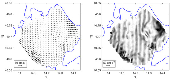
Figure 1.
Surface currents data provided by the HF radar system in the Gulf of Naples (on the left) and the interpolated data (on the right). Black arrows denote the velocity field whereas the blue line represents the coastline.
With a reference velocity scale U of , a length scale L of and a Coriolis parameter , the Rossby number is . It is thus evident that the quasi-geostrophic equations are not accurate for describing the GoN dynamics.
2.2. Dynamical Parameters Characterizing Recirculations
At a first glance, eddies of two-dimensional turbulent flows can be described as flow regions characterized by a rigid-body rotation. In this approximation, many local and semi-local parameters can be adopted to decide whether vortices exist or are likely to develop. As eddies are extensive structures, it is natural to consider integral quantities, rather than pointwise ones, to identify them. Nevertheless, the choice of the appropriate computational regions, specifically their shape and area, is completely arbitrary. For this reason these parameters naturally depend on a scale coefficient.
2.2.1. Okubo–Weiss and Local Okubo–Weiss Parameters
The Okubo–Weiss parameter () is a local dynamical field which, loosely speaking, measures the relative dominance of the rate-of-strain tensor s over the vorticity of the velocity field (here denotes the euclidean module)
It was independently introduced by [39,40]. For a two-dimensional flow it turns out that
By definition whenever the rotation tendency exceeds the strain one.
The local version of the parameter, called the local Okubo–Weiss parameter (see [10]), depends on a positive distance and is defined as the integral of over the disk of radius a:
2.2.2. Local Normalized Angular Momentum and Momentum Flux Fields
In the rotating rigid-body analogy the angular momentum of a fluid particle has to be maximized about the eddy center, as pointed out by [41]. This consideration suggested to define the local normalized angular momentum field :
which assumes extreme values at the centers of circular symmetric eddies: for cyclonic rotations and for anticyclonic ones (in [41] the term appears with its sign; we added the modulus to get .)
Analogously, the local normalized momentum flux field can be defined as follows:
It is clear that identically vanishes on centers of rotating eddies, while it assumes extreme values at the symmetric sources and sinks; so it can be adopted to distinguish these various types of recirculating structures.
3. Methods
3.1. Eddy Detection Algorithms
We implemented two versions of two different existing detection algorithms for our study. The first method, the angular momentum eddy detection and tracking algorithm (AMEDA), developed by [10], was tested on several products such as altimeter data, numerical simulations and laboratory experiment. The second, proposed by [11], the ’Nencioli et al. algorithm’ (NEAL), was specifically designed for certain HF radar derived datasets.
It is worth noting that in both cases above the velocity fields utilized for testing and application were geostrophic or quasi-geostrophic. On the other hand the surface flow observed in the GoN is highly non-geostrophic and significant variations of the divergence field frequently occur, often associated to recirculating sources or sinks. So, to distinguish similar structures in our study area, it was necessary to modify those algorithms, and yet, as discussed in the following, our proposed refinements led to just moderate improvements. Therefore, in order to specifically address the aforementioned classification problems, we defined a third method, yet another eddy detection algorithm (YADA), inspired by [10,12].
3.2. Ameda
The AMEDA algorithm ([10]) determines the eddy centers accordingly with the following procedure:
- 1.
- Identifies grid points which are local extrema of satisfying and , for a chosen threshold ;
- 2.
- Verifies the existence of at least one closed streamline around each extremum.
However, as already pointed out, GoN eddies may have hyperbolic orbits, in contrast with the geostrophic flows found in [10,11]. In such cases the second assumption is never verified, so we decided to adopt the following alternative criterion (described in [11]):
- 2’.
- Confirms that the velocity field constantly rotates along the perimeter of the square domain of edge and centered at the extremum, for a chosen distance b.
The modified version of AMEDA, obtained by substituting 2 with 2’, is here denoted by AMEDAmod.
3.3. Neal
The eddy detection algorithm developed in [11], and here denoted by NEAL, identifies the eddy centers in several steps, namely:
- 1.
- Identifies couples of adjacent grid points such that the meridional component of the velocity field changes sign going westward along the zonal segment of length , centered at , and increases its magnitude away from this point. This computation also provides the expected sign of rotation;
- 2.
- Verifies that, at any such grid point , the zonal component of the velocity field changes sign going northward along the meridional segment of length , centered at , and increases its magnitude away from this point. This change must be compatible with the expected rotation;
- 3.
- Identifies the (kinetic energy) local minima inside a square domain of edge , centered at , which are global minima in a square neighborhood of the same size;
- 4.
- Confirms that the velocity field constantly rotates along the perimeter .
3.4. Yada
The YADA algorithm searches for potential eddy centers in two steps:
- 1.
- Identifies the local extrema of a dynamical field like , or ;
- 2.
- Analyzes the streamline geometry within some neighborhood of each extremum, ensuring the existence of either bounded hyperbolic orbits (characterizing eddies with sink-like cores) or elliptic orbits (in presence of eddies having stable orbits).
Note that the second step is precisely designed to distinguish different eddy geometries. During this classification procedure, as we will see in the next section, the YADA algorithm computes quantities that are strongly related to the eddy shape, and therefore provide useful information about its character, which may be either hyperbolic or elliptic, depending on the streamline behavior.
3.5. Tuning Strategy
Each algorithm depends on some parameters, specifically the threshold and the neighborhood radii a and b, which have to be tuned in order to maximize the probability of detection. In principle, such a training phase should be carried out with a set of completely characterized observations, for which the real eddy population and its spatio-temporal distribution is perfectly known. This is never the case for eddy detection studies. In [10] the authors, in order to cross-validate their parametric algorithm, considered the number of detected eddies as a score function depending on the algorithm parameters. The best model was then chosen by looking for parameters stabilizing the score function. The reasoning behind this approach can be heuristically described as follows. One starts with an inaccurate model which predicts too few (or too many) eddies. However, by randomly exploring different parameter values, one may observe an increase (decrease) of the score function until reaching a stable region in the parameter space. Then, elements within the stable region can be considered optimal assuming that the observed local fluctuations are caused by the existence of eddies, that randomly fall in (or escape from) the detection range as parameters vary. In our study we chose to adopt the same tuning strategy, better described in the next section.
4. Results
In this section we first describe the tuning procedure for each chosen algorithm and then we discuss the results. Before doing this, some observations about the algorithm definitions are needed. Firstly, for numerical convenience, we substituted the disk in the definition of and with the square domain centered at of edge , which we denote by . Secondly, we note that in both algorithms AMEDA and NEAL the final step concerns the rotation of the velocity vector along a boundary profile. This was explicitly done by following the path counter-clockwise and verifying that any velocity vector at a given grid point was rotated to the left of the previous by an angle less than radians; note that this criterion does not depend on the sense of rotation of the velocity field along the path.
4.1. Ameda Tuning and Results
Three parameters have to be determined to run this algorithm: a, from the definition of and , and b. To obtain all dimensionless parameters we divided a and b by the length scale l of one pixel ( km): and .
The optimal choice of these parameters depends on the scale analysis of the investigated dynamics: if is too large then may sum up the contribution of many eddies inside , leading to a wrong estimate of the angular momentum. Similarly a large is not recommended, nor is a small one since the velocity vector may abruptly rotate with an angular velocity greater than radians per pixel in proximity of the eddy center. The parameter , in turn, once is coherently chosen, represents a lower bound for the detected eddy intensity.
We ran the algorithm on the 10-day dataset described in Section 2.1 for different values of the parameters and , and analyzed the number of detected eddies as a function of , varying from to 1 with step . The results are shown in Figure 2.
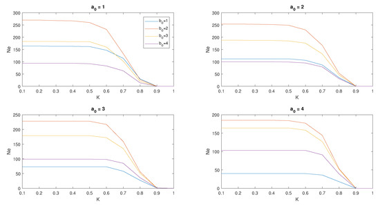
Figure 2.
Number of eddies detected in the observation period , obtained with the angular momentum eddy detection and tracking algorithm (AMEDA) for different values of the parameters , and . In each figure, corresponding to a value of , the colored curves denote the graphs of as a function of for different values of (labeled as in the legend).
For any choice of and the values of turned out to be approximately constant for , so we set . On the other hand for a fixed the maximum of was achieved at ; so we chose this value for . Finally we noted that weakly decreased as increased, as expected, suggesting to take . In summary, our optimal choice of the parameters turned out be .
Since we were interested in discriminating diverging structures from converging ones we added a third control to AMEDA (see above, Section 3.4):
- 3.
- Discards those extrema satisfying .
In this way we allowed only a little divergence near the eddy core (see the contour line in Figure 3 for instance). This correction reduced the number of detected eddies by about 16% for , and by 0.4% for ; this behavior was expected since strong rotations often imply weak divergences.
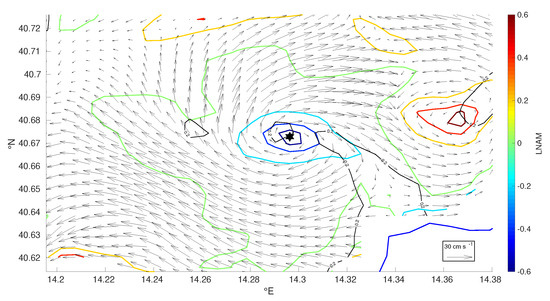
Figure 3.
Source-like eddy core detected by the algorithm AMEDA (black star), velocity field (black arrows), local normalized angular momentum field contour lines (colored), local normalized momentum flux = contour (black lines) and coastline (blue line).
Unfortunately this criterion is not optimal: It is a pure dynamical control depending on the local behavior of the flow, but eddies are extensive structures which may admit internal divergences. In such a case the eddy center and its real extension is difficult to estimate since it would be necessary to understand the streamline geometry.
4.2. Neal Tuning and Results
By definition NEAL is a purely geometrical method, which is not required to compute any differential quantity: Eddy centers are simply defined as energy minima. Of course this reduces the computation time, making the algorithm fast and efficient. Moreover we note that, as in the previous case, there are two parameters, a and b, to be determined; as before we considered the dimensionless parameters and .
We ran the algorithm on the dataset for and . In Figure 4 the number of eddies , discarding the unlikely results obtained for (), is shown. We observed that for there was a weak dependence on , but the values of turned out to be much less than those obtained by AMEDA. For the number of detected eddies highly depended on , but the results did not converge anywhere; for we obtained values depending weakly on but much less than those for . These discrepancies were likely caused by asymmetrical eddies lacking radially increasing velocity components. In conclusion, we were not able to tune NEAL, as no stable regions in the parameter space were identified.
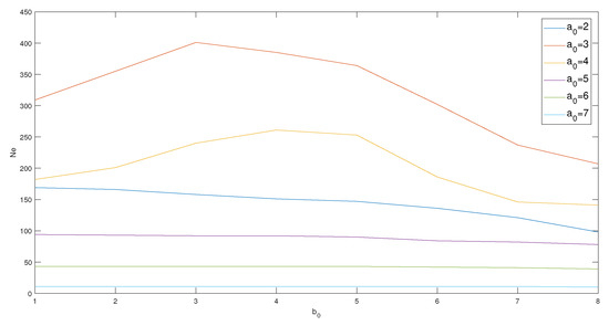
Figure 4.
Number of eddies detected in the observation period, , obtained by the ’Nencioli et al. algorithm’ (NEAL) for different choices of the parameters and . Colored lines denote the graphs of as a function of for different values of (labeled as in the legend).
4.3. Yada Tuning and Results
The first step of the algorithm coincides with that of AMEDA: it identifies any local extremum of satisfying for (having tested this values in tuning AMEDA).
The second step concerns the study of the streamline geometry in a neighborhood of the extremum. It proceeds as follows: in a square neighborhood centered at with edge , where the length b has to be intended as an upper limit for the eddy radius (which, in this study, has been overestimated to be ), it draws a circle of radius , centered at and composed by 8 points (as many as the grid points on the tangent square perimeter). It then computes the streamlines originated from these points (each streamline is built by means of a fourth order Runge–Kutta method, with a step of 5 points per pixel. It is composed by up to 1000 points), collecting their mean points (geometric means) and end points.
Then the algorithm performs a selection of all the streamlines such that:
- (1)
- The end points belong to the square domain (that is: they stay away from the boundary of the reference domain);
- (2)
- Each streamline completes at least one revolution.
The second control consists in looking at the cumulative winding-angle (given an oriented piece-wise linear curve, its cumulative winding-angle is the sum, over all the angular points, of the angle, with positive sign going counter-clockwise and negative going clockwise, between the two intersecting segments, considered as vectors) of the streamline, as defined in [12]: it has to be, in modulus, equal to or grater than . If no such streamline exists we increase the radius of by l until at least one streamline satisfying (1) and (2) is found; the maximum allowed r will be (at any step we increase the number of points in the circle to match the amount of grid points in the tangent square perimeter).
Note that if one such streamline exists it means that either it converges to some point inside the domain or it definitely stays inside the domain without converging anywhere (at least for the first 1000 points). Of course some diverging streamline, which rotates without reaching the boundary of the domain, could exist and be identified by the algorithm. However, a path starting from and which rotates around it at least three times before reaching the boundary, and having the same step-size of the drawn streamlines, counts approximately 300–400 points. Then, if a spiral-like streamline diverging from the center stays inside the domain without reaching the boundary, it has to complete at least eight revolutions; even in this case we can safely affirm that an eddy exists.
Once the algorithm has selected all the streamlines satisfying (1) and (2) for the first allowable r, it compares the distributions of the mean points with that of the end points. If the eddy core behaves as a sink all the end points will accumulate near it. On the other hand if the orbits around the eddy are elliptic the mean points will be close to the orbits’ common center of mass. So the algorithm chooses the distribution with less variance and choose its mean point as eddy center of mass, or eddy symmetry center (ESC); by contrast the extremum will be called the eddy extreme point (EEP). However, to ensure it is not selecting another eddy in the square domain relative to a different extremum, it is required that the expected ESC must belong to the disk bounded by , otherwise the point is discarded and the algorithm moves toward the next extremum; some examples of this procedure can be found in Figure 5 and Figure 6.
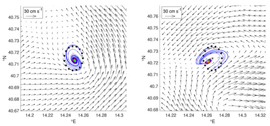
Figure 5.
Maps showing the functioning of ’yet another eddy detection algorithm’ (YADA) for two eddies with sink-like cores. Once the eddy extreme point (EEP) (black crosses) is detected, YADA identifies a circle (black stars), centered at the extremum, which emanates streamlines (blue lines) with the following property: The streamline has to complete up to a revolution without reaching the domain boundary. Then it evaluates the mean points (yellow stars) and end points (red stars) of such streamlines, choosing the mean point of the second distribution as eddy symmetry center (ESC) (green stars). Black arrows denote the velocity field. In both panels the mean point and the ESC coincide.
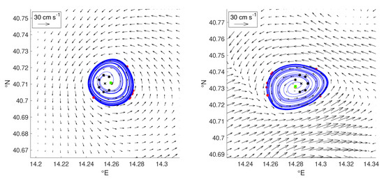
Figure 6.
Maps showing the functioning of YADA for two eddies having elliptic orbits. Once the eddy extreme point EEP (black crosses) is detected, YADA identifies a circle (black stars) emanating streamlines (blue lines) with the following property: Each streamline has to complete up to a revolution without reaching the domain boundary. Then it evaluates the mean points (yellow stars) and end points (red stars) of such streamlines, choosing the mean point of the first distribution as eddy symmetry center ESC (green stars). Black arrows denote the velocity field. In both panels the mean point and the ESC coincide.
Generally the does not coincide with the eddy center even though it provides a better approximation of the true eddy core than the ; e.g., Figure 5, Figure 6, Figure 7 and Figure 8. As a consequence the distance between the ESC and the EEP can be considered as a measure of the eddy asymmetry.
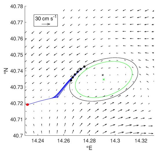
Figure 7.
Map showing the YADA boundary computation of an eddy having a sink-like core. Once the eddy extreme point EEP (black cross) and the eddy symmetry center ESC (green cross) are detected the algorithm draws the ellipses centered at the ESC with increasing radii. The cycle breaks when the black ellipse is drawn due to the existence of inadmissible streamlines (blue lines) leaving the domain. The last computed ellipse (green line) will be considered as boundary. Black arrows denote the velocity field.
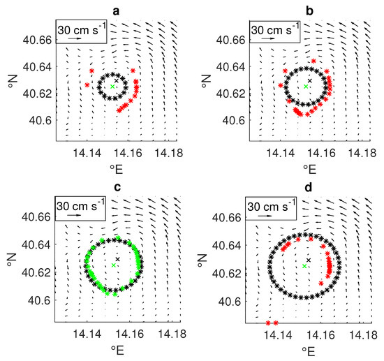
Figure 8.
Maps showing the YADA boundary computation of an eddy having stable orbits. From panel (a–d) ellipses of increasing semi-major axes are drawn; the temporal frame is unchanged. Once the EEP (black crosses) and the ESC (green crosses) are detected the algorithm draws the ellipses centered at the ESC with increasing semi-major axis d (black stars); from panels (a–d) the semi-major axis increases from 2 to 5 pixel lengths. It then evaluates the end points (red stars in panels (a,b,d), and green stars in (c)) of the streamlines emanated by these ellipses. The algorithm selects the semi-major axis for which the relative end points (green stars in (c)) form the closest deformation of the associated ellipse. Black arrows denote the velocity field.
Following the procedure just described, the algorithm detected eddies, about 30% more than the value obtained with AMEDA. Eddies such as those in Figure 5, for instance, were missed by AMEDA due to their small extension and asymmetry, whereas they were detected by YADA. However there were still structures detected by AMEDA and missed by YADA, see for instance Figure 9. In some of these cases we noted that the divergence around the extremum was so weak () that some orbits complete up to three revolutions before leaving the region.
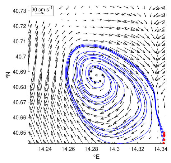
Figure 9.
Eddy detected by AMEDA and missed by YADA. The local normalized angular momentum field extremum x (black cross) corresponds to an eddy core, but any circle centered at x (black stars) emanates streamlines (blue lines) which complete up to 3 revolutions before reaching the domain boundary (contact points in red). Black arrows denote the velocity field.
In conclusion we can affirm that YADA was able to detect and distinguish multiple kinds of eddies and, as it will be shown in the next part, it can be refined to estimate their boundaries.
4.4. Eddy Boundaries
There is no universal definition of eddy boundary: many authors adopted or contour lines, as well as closed streamlines or closed stream-function contours (not equivalent at all) to locate them.
Based on YADA architecture, we propose a different definition, which aims to distinguish eddies with sink-like cores from those having elliptic orbits. Of course we can not expect to identify the true boundary profile, so we assume it to be in general elliptic (rather than circular).
4.4.1. Sink-Like Cores
We considered the set of all the streamlines originated from and satisfying conditions (1) and (2) as explained in the definition of YADA. We then evaluated the variance ellipse of this distribution of points; let e be its eccentricity. Then we drew the ellipse of eccentricity e, centered at the , with major semi-axis . As we did for we consider the streamlines emanated by and if all such streamlines belong to the ellipse interior we increment d by l, repeating the step up to reach . Further, in analogy with [10], we also control that the circulation along does not decrease by increasing d. The largest ellipse satisfying this criterion will define the eddy boundary, as shown in Figure 7.
4.4.2. Eddies Having Elliptic Orbits
For such eddies we also started by building the variance ellipse of the admissible streamlines . Then we drew the ellipses with eccentricity e, centered at the ESC and having semi-major axis , where was the maximum distance for which the circulation around was a non-decreasing function of d, and we moved each following the flow, thus collecting all the end points of the streamlines emanated by . We denoted this set by .
We expected that, if approximated the eddy boundary, it had to be close to an elliptic orbit, and therefore had to be a small deformation of . However, in order to ignore the effects of translating motions, which could occur, we centered the two sets on the same reference point. Then we evaluated the Hausdorff distance between them (see the Appendix A for details).
Finally we took satisfying , and as eddy boundary; we chose to keep the elliptic symmetric, though would provide a better approximation. In Figure 8 we plotted the various steps just described; in each panel the ellipse of semi-major axis is drawn.
5. Discussion
5.1. Detected Eddies
In Section 4 we tried to tune the three chosen algorithms by following a stability criterion. We succeeded for AMEDA, but failed for NEAL. Indeed, in the latter case, no stable parameter regions were identified. The algorithm YADA, instead, was indirectly tuned by using the AMEDA common parameters, namely K and a; in fact both these parameters served to set a lower bound to the eddy rotational energy, which was independent on the algorithm itself.
We then compared the tuned version of the two algorithms, AMEDA and YADA. It turns out that AMEDA detected 195 eddies within the time period, whereas YADA detected 255 eddies. However, among these, 157 eddies have been identified by both, leaving 38 eddies detected by AMEDA but missed by YADA and 98 seen by YADA but lost by AMEDA. Mismatches between AMEDA and YADA detections were expected, as already observed: eddies like that in Figure 9 were missed by YADA due to their large extension and weak, but still positive, divergence. On the other hand, deformed recirculations, as in Figure 5, were easily hidden to AMEDA but not to YADA.
Finally we checked by visual inspection all the available time frames, in order to determine the existence of false positive detections. Interestingly, no such detections were found, testifying the reliability of both the algorithms, at least in terms of false alarms. The same inspection showed that volatile and higly asymmetrical structures were still missed by both. However, our algorithm was able to detect long-lived eddies for longer time periods, as shown in Figure 10.
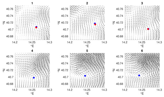
Figure 10.
Sequence of time frames (from panel 1 to 6) showing the evolution of a detected eddy. Red stars denote eddy centers identified by AMEDA, whereas blue stars indicate ESCs computed by YADA. As the eddy changes shape and becomes less centrosymmetric AMEDA misses it (panel 3 to 4). Black arrows denote the velocity field (not in scale).
5.2. Equivalent Radii
Following [10] we computed the equivalent radius for each detected eddy. It is defined as the radius of the circle bounding an area equivalent to that delimited by the eddy boundary. For elliptic contours it equals . The mean radius turned out to be km, with a standard deviation of km and values of and km for the 95th and 99th percentile respectively. Similarly we computed a mean eccentricity of with standard deviation of . It turned out that the mean equivalent radius was merely 1–2 times the pixel length scale of the dataset, and therefore we could expect that our method would not accurately describe some kinematic and dynamic features of eddies having close to . It may have been possible to obtain a more accurate description by increasing the spatial resolution up to reach km; however this would have implied performing interpolations at a much higher resolution.
5.3. Spatial Distribution
The hourly sampling frequency of the HF radar allowed to track eddies having longer lifetime. We identified such long-lived structures by looking for eddies encircling an EEP, coming from the previous temporal frame, within their own boundary. The spatial distribution of all the detected long-lived eddies, counted without repetitions, can be found in Figure 11.
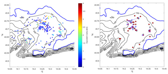
Figure 11.
Left panel: Spatial distribution of the detected eddies by means of YADA (colored circles); different colors denote different sizes. Right panel: Detected long-lived eddies (circles) with lifetime h. Initial, mid and final EEPs (black circles, blue circles and red stars respectively) with their relative eddy trajectories (blue dashed lines) and eddy lifetimes h (blue numbers). Shoreline (blue contour) and bathymetric contour lines (black lines) between 100 m and 800 m of depth.
A larger density can be noted in correspondence of a relatively flat plateau located in N, E, between 120 and 160 m of depth, excluding topographic wakes, that need steep bathymetric slopes, as primary instability causes (for a comprehensive analysis of several submesoscale eddy generation mechanisms see [5]). To understand the instability sources generating the GoN eddies, therefore, it would be necessary to investigate the flow behavior within the SBL (surface boundary layer). Unfortunately there are neither wind observations nor density profiles relative to the GoN SBL. However, there is a work in progress, funded by the Science and Technology department of the Parthenope University of Naples, aiming to investigate the vertical water profile through numerical simulation. Such a study could provide more information to understand the instability sources within the GoN.
Finally we observed that the detected long-lived eddies, namely those with lifetimes greater than 1 h, were 36, distributed as shown in Figure 11. They usually persisted for few hours, 5 or 7 h in some cases, distributed in agreement with the entire density population. We also noted that, except for few examples, they were almost stationary.
6. Conclusions
Submesoscale motions play an important role in the transfer of energy from the mesoscale down to the dissipative range ([5,42]) as well as in the transport of pollutants, of biomass, of organic and inorganic matter ([43,44]). At present, they represent one of the frontiers of the study of transport in the ocean. On the other hand, as recently pointed out by several authors (see, e.g., [5,8,45]), the observation of submesoscale eddies in a synoptic way is challenging, feasible with remote sensing techniques which are typicaly limited by available resolution. HF radars are land-based remote sensing tools that can be very suitable for such investigations, given their temporal and spatial sampling characteristics. In this paper we have tackled the issue of devising an algorithm for submesoscale eddy detection in a high resolution surface velocity field provided by a network of 25 Mhz coastal radar antennas active in the Gulf of Naples. We started by applying two different eddy detection algorithms, here denoted by AMEDA and NEAL, based on the studies of [10,11] respectively, but they both displayed some weaknesses. The application of AMEDA to the selected surface current dataset demonstrated to be unable to distinguish submesoscale eddies entrapping fluid masses from the others. So we refined the algorithm by measuring the divergence occurring in the eddy core. The number of detected eddies then decreased. Differently, we did not succeed to tune the algorithm NEAL.
To obtain a more efficient detection method, able to distinguish asymmetric eddies entrapping fluid masses, we developed a novel, modified algorithm, named YADA, which detected 255 eddies (about 30% more than the refined AMEDA value). Then we used YADA to estimate the eddy boundaries, assuming an elliptical symmetry, and we found a mean equivalent radius of km and a mean eccentricity of .
YADA’s results were validated comparison with the results of the algorithm AMEDA, as well as by visual inspection of all time frames. Having developed a more robust algorithm, this also allowed us to look at the spatial distribution of the detected eddies, and to observe a larger density at the plateau located at 160 m of depth, and led us to exclude topographic wakes as main instability sources. Moreover, we obtained estimates for their spatial scales taking into account the noncircular geometry of the vortices.
As mentioned above, submesoscale eddies represent a relevant transport mechanism for waters and their biogeochemical characteristics; their influence is particularly important in those coastal areas, such as the Gulf of Naples, characterized by the coexistence of different subsystems, whose mutual exchanges may strongly affect the whole functioning of the area. For this reason an accurate identification of such structures is a necessary first step for the quantitative assessment of their role, which we plan to further investigate in terms of their specific transport properties both in the horizontal and in the vertical.
Author Contributions
Conceptualization L.B., P.F. and E.Z.; methodology L.B., P.F. and E.Z.; formal analysis L.B., P.F. and E.Z.; writing–review and editing L.B., P.F. and E.Z.; data curation L.B.; funding acquisition E.Z. and P.F. All authors have read and agreed to the published version of the manuscript.
Funding
E.Z. acknowledges support from the Parthenope University of Naples internal research fund; this work was partially supported by “DORA - Deployable Optics for Remote sensing Applications DORA” (ARS01_00653), a project funded by MIUR - PON “Research & Innovation”/PNR 2015-2020.
Acknowledgments
The Department of Sciences and Technologies (formerly the Department of Environmental Sciences) of the Parthenope University of Naples operates the HFR system on behalf of the AMRA consortium (formerly CRdC AMRA), a regional competence center for the analysis and monitoring of environmental risks. Our radar remote sites are hosted by the ENEA Centre of Portici, the ‘Villa Angelina Village of High Education and Professional Training’, ‘La Villanella’ resort in Massa Lubrense and the Fincantieri shipyard in Castellammare di Stabia, whose hospitality is gratefully acknowledged. The authors would like to thank Angelo Perilli for useful conversations and Teresa Hann for her help in reviewing the manuscript.
Conflicts of Interest
The authors declare no conflict of interest.
Appendix A. the Hausdorff Distance
The Hausdorff distance between two compact subsets A and B of the euclidean plane is defined by the formula
where and are the usual point-set distances:
The Hausdorff distance makes the set of all compact subsets a metric space; in particular if and only if .
References
- Cushman-Roisin, B.; Gualtieri, C.; Mihailovic, D.T. Environmental Fluid Mechanics: Current issues and future outlook. In Fluid Mechanics of Environmental Interfaces; Taylor & Francis: Abingdon UK, 2008; pp. 17–30. [Google Scholar]
- Zambianchi, E.; Griffa, A. Effects of finite scales of turbulence on dispersion estimates. J. Mar. Res. 1994, 52, 129–148. [Google Scholar] [CrossRef]
- Haza, A.C.; Özgökmen, T.M.; Griffa, A.; Garraffo, Z.D.; Piterbarg, L. Parameterization of particle transport at submesoscales in the Gulf Stream region using Lagrangian subgridscale models. Ocean. Model. 2012, 42, 31–49. [Google Scholar] [CrossRef]
- McWilliams, J.C. Submesoscale, coherent vortices in the ocean. Rev. Geophys. 1985, 23, 165–182. [Google Scholar] [CrossRef]
- McWilliams, J.C. Submesoscale currents in the ocean. Proc. R. Soc. A 2016. [Google Scholar] [CrossRef] [PubMed]
- Lévy, M.; Franks, P.J.; Smith, K.S. The role of submesoscale currents in structuring marine ecosystems. Nat. Commun. 2018, 9, 1–16. [Google Scholar] [CrossRef] [PubMed]
- Mahadevan, A. The impact of submesoscale physics on primary productivity of plankton. Annu. Rev. Mar. Sci. 2016, 8, 161–184. [Google Scholar] [CrossRef]
- Poje, A.C.; Özgökmen, T.M.; Lipphardt, B.L.; Haus, B.K.; Ryan, E.H.; Haza, A.C.; Jacobs, G.A.; Reniers, A.; Olascoaga, M.J.; Novelli, G.; et al. Submesoscale dispersion in the vicinity of the Deepwater Horizon spill. Proc. Natl. Acad. Sci. USA 2014, 111, 12693–12698. [Google Scholar] [CrossRef]
- Doglioli, A.M.; Blanke, B.; Speich, S.; Lapeyre, G. Tracking coherent structures in a regional ocean model with wavelet analysis: Application to Cape Basin eddies. J. Geophys. Res. Ocean. 2007, 112, C5. [Google Scholar] [CrossRef]
- Le Vu, B.; Stegner, A.; Arsouzea, T. Angular Momentum Eddy Detection and tracking Algorithm (AMEDA) and its application to coastal eddy formation. Atmos. Ocean. Technol. 2017, 35, 739–762. [Google Scholar] [CrossRef]
- Nencioli, F.; Dong, C.; Duckey, T.; Washburn, L.; McWilliams, J.C. A Vector Geometry Based Eddy Detection Algorithm and Its Application to a High-Resolution Numerical Model Product and High-Frequency Radar Surface Velocities in the Southern California Bight. Atmos. Ocean. Technol. 2008, 27, 564–579. [Google Scholar] [CrossRef]
- Post, F.H.; Sadarjoen, I.A. Detection, quantification, and tracking of vortices using streamline geometry. Comput. Graph. 2000, 24, 333–341. [Google Scholar]
- Pessini, F.; Olita, A.; Cotroneo, Y.; Perilli, A. Mesoscale eddies in the Algerian Basin: do they differ as a function of their formation site? Ocean. Sci. 2018, 14, 5. [Google Scholar] [CrossRef]
- Chelton, D.B.; DeSzoeke, R.A.; Schlax, M.G.; El Naggar, K.; Siwertz, N. Geographical variability of the first baroclinic Rossby radius of deformation. J. Phys. Oceanogr. 1998, 28, 433–460. [Google Scholar] [CrossRef]
- Lévy, M.; Klein, P.; Treguier, A.M. Impact of sub-mesoscale physics on production and subduction of phytoplankton in an oligotrophic regime. J. Mar. Res. 2001, 59, 535–565. [Google Scholar] [CrossRef]
- Grilli, F.; Pinardi, N. The computation of Rossby radii of deformation for the Mediterranean Sea. MTP News 1998, 6, 4–5. [Google Scholar]
- Pinardi, N.; Masetti, E. Variability of the large scale general circulation of the Mediterranean Sea from observations and modelling: a review. Palaeogeogr. Palaeoclimatol. Palaeoecol. 2000, 158, 153–173. [Google Scholar] [CrossRef]
- Corrado, R.; Lacorata, G.; Palatella, L.; Santoleri, R.; Zambianchi, E. General characteristics of relative dispersion in the ocean. Sci. Rep. 2017, 7, 46291. [Google Scholar] [CrossRef]
- Rubio, A.; Mader, J.; Corgnati, L.; Mantovani, C.; Griffa, A.; Novellino, A.; Quentin, C.; Wyatt, L.; Schulz-Stellenfleth, J.; Horstmann, J.; et al. HF radar activity in European coastal seas: next steps toward a pan-European HF radar network. Front. Mar. Sci. 2017, 4, 8. [Google Scholar] [CrossRef]
- Paduan, J.D.; Washburn, L. High-Frequency Radar Observations of Ocean Surface Currents. Annu. Rev. Mar. Sci. 2013, 5, 115–136. [Google Scholar] [CrossRef]
- Karimova, S.; Gade, M. Eddies in the Western Mediterranean seen by spaceborne radar. In Proceedings of the 2016 IEEE International Geoscience and Remote Sensing Symposium (IGARSS), Beijing, China, 10–15 July 2016; pp. 3997–4000. [Google Scholar]
- Karimova, S.; Gade, M. Improved statistics of sub-mesoscale eddies in the Baltic Sea retrieved from SAR imagery. Int. J. Remote. Sens. 2016, 37, 2394–2414. [Google Scholar] [CrossRef]
- Karimova, S.S.; Gade, M. Eddies in the Red Sea as seen by satellite SAR imagery. In Remote Sensing of the African Seas; Springer: Berlin/Heidelberg, Germany, 2014; pp. 357–378. [Google Scholar]
- Menna, M.; Mercatini, A.; Uttieri, M.; Buonocore, B.; Zambianchi, E. Wintertime transport processes in the Gulf of Naples investigated by HF radar measurements of surface currents. Nuovo Cimento C 2007, 30, 605–622. [Google Scholar]
- Cianelli, D.; Falco, P.; Iermano, I.; Mozzillo, P.; Uttieri, M.; Buonocore, B.; Zambardino, G.; Zambianchi, E. Inshore/offshore water exchange in the Gulf of Naples. J. Mar. Syst. 2015, 145, 37–52. [Google Scholar] [CrossRef]
- Carrada, G.C.; Hopkins, T.S.; Bonaduce, G.; Ianora, A.; Marino, D.; Modigh, M.; Ribera D’Alcalà, M.; di Scotto, C.B. Variability in the hydrographic and biological features of the Gulf of Naples. Mar. Ecol. 1980, 1, 105–120. [Google Scholar] [CrossRef]
- Cianelli, D.; Uttieri, M.; Buonocore, B.; Falco, P.; Zambardino, G.; Zambianchi, E. Dynamics of a very special Mediterranean coastal area: the Gulf of Naples. In Mediterranean Ecosystems: Dynamics, Management and Conservation; Nova Science: Hauppauge, NY, USA, 2012; pp. 129–150. [Google Scholar]
- Moretti, M.; Sansone, E.; Spezie, G.; Vultaggio, M.; De Maio, A. Alcuni aspetti del movimento delle acque del Golfo di Napoli. Annali Ist Univ Nav XLV-XLVI 1976, 207–217. [Google Scholar]
- De Maio, A.; Moretti, M.; Sansone, E.; Spezie, G.; Vultaggio, M. Outline of marine currents in the Bay of Naples and some considerations on pollutant transport. Il Nuovo Cimento C 1985, 8, 955–969. [Google Scholar] [CrossRef]
- Uttieri, M.; Cianelli, D.; Nardelli, B.B.; Buonocore, B.; Falco, P.; Colella, S.; Zambianchi, E. Multiplatform observation of the surface circulation in the Gulf of Naples (Southern Tyrrhenian Sea). Ocean. Dyn. 2011, 61, 779–796. [Google Scholar] [CrossRef]
- De Ruggiero, P.; Esposito, G.; Napolitano, E.; Iacono, R.; Pierini, S.; Zambianchi, E. Modelling the marine circulation of the Campania Coastal System (Tyrrhenian Sea) for the year 2016: Analysis of the dynamics. J. Mar. Syst. 2019. Submitted. [Google Scholar]
- D’Alelio, D.; Mazzocchi, M.G.; Montresor, M.; Sarno, D.; Zingone, A.; Di Capua, I.; Franzè, G.; Margiotta, F.; Saggiomo, V.; Ribera d’Alcalà, M. The green-blue swing: plasticity of plankton food-webs in response to coastal oceanographic dynamics. Mar. Ecol. 2015, 36, 1155–1170. [Google Scholar] [CrossRef]
- Cianelli, D.; D’Alelio, D.; Uttieri, M.; Sarno, D.; Zingone, A.; Zambianchi, E.; d’Alcalà, M.R. Disentangling physical and biological drivers of phytoplankton dynamics in a coastal system. Sci. Rep. 2017, 7, 15868. [Google Scholar] [CrossRef]
- Sciascia, R.; Berta, M.; Carlson, D.F.; Griffa, A.; Panfili, M.; Mesa, M.L.; Corgnati, L.; Mantovani, C.; Domenella, E.; Fredj, E.; et al. Linking sardine recruitment in coastal areas to ocean currents using surface drifters and HF radar: A case study in the Gulf of Manfredonia, Adriatic Sea. Ocean. Sci. 2018, 14, 1461–1482. [Google Scholar] [CrossRef]
- Iermano, I.; Moore, A.; Zambianchi, E. Impacts of a 4-dimensional variational data assimilation in a coastal ocean model of southern Tyrrhenian Sea. J. Mar. Syst. 2016, 154, 157–171. [Google Scholar] [CrossRef]
- Kalampokis, A.; Uttieri, M.; Poulain, P.M.; Zambianchi, E. Validation of HF radar-derived currents in the Gulf of Naples with Lagrangian data. IEEE Geosci. Remote Sens. Lett. 2016, 13, 1452–1456. [Google Scholar] [CrossRef]
- Ranalli, M.; Lagona, F.; Picone, M.; Zambianchi, E. Segmentation of sea current fields by cylindrical hidden Markov models: a composite likelihood approach. J. R. Stat. Soc. Ser. Appl. Stat. 2018, 67, 575–598. [Google Scholar] [CrossRef]
- Saviano, S.; Kalampokis, A.; Zambianchi, E.; Uttieri, M. A year-long assessment of wave measurements retrieved from an HF radar network in the Gulf of Naples (Tyrrhenian Sea, Western Mediterranean Sea). J. Oper. Oceanogr. 2019, 12, 1–15. [Google Scholar] [CrossRef]
- Okubo, A. Horizontal dispersion of floatable trajectories in the vicinity of velocity singularities such as convergencies. Deep-Sea Res. 1970, 17, 445–454. [Google Scholar]
- Weiss, J. The dynamics of enstrophy transfer in 2-dimensional hydrodynamics. Phys. D 1991, 48, 273–294. [Google Scholar] [CrossRef]
- Mkhinini, N.; Coimbra, A.L.S.; Stegner, A.; Arsouze, T.; Taupier-Letage, I.; Béranger, K. Long-lived mesoscale eddies in the eastern Mediterranean Sea: Analysis of 20 years of AVISO geostrophic velocities. J. Geophys. Res. Oceans 2014, 119, 8603–8626. [Google Scholar] [CrossRef]
- Ferrari, R.; Wunsch, C. Ocean circulation kinetic energy: Reservoirs, sources, and sinks. Annu. Rev. Fluid Mech. 2009, 41, 253–282. [Google Scholar] [CrossRef]
- Lévy, M.; Ferrari, R.; Franks, P.J.; Martin, A.P.; Rivière, P. Bringing physics to life at the submesoscale. Geophys. Res. Lett. 2012, 39, 14. [Google Scholar] [CrossRef]
- Smith, K.M.; Hamlington, P.E.; Fox-Kemper, B. Effects of submesoscale turbulence on ocean tracers. J. Geophys. Res. Ocean. 2016, 121, 908–933. [Google Scholar] [CrossRef]
- Schroeder, K.; Chiggiato, J.; Haza, A.; Griffa, A.; Özgökmen, T.; Zanasca, P.; Molcard, A.; Borghini, M.; Poulain, P.M.; Gerin, R.; et al. Targeted Lagrangian sampling of submesoscale dispersion at a coastal frontal zone. Geophys. Res. Lett. 2012, 39, 11. [Google Scholar] [CrossRef]


© 2019 by the authors. Licensee MDPI, Basel, Switzerland. This article is an open access article distributed under the terms and conditions of the Creative Commons Attribution (CC BY) license (http://creativecommons.org/licenses/by/4.0/).