Abstract
Great Barrier Reef catchments are under pressure from the effects of climate change, landscape modifications, and hydrology alterations. With the use of remote sensing datasets covering large areas, conventional methods of change detection can expose broad transitions, whereas workflows that excerpt data for time-series trends divulge more subtle transformations of land cover modification. Here, we combine both these approaches to investigate change and trends in a large estuarine region of Central Queensland, Australia, that encompasses a national park and is adjacent to the Great Barrier Reef World Heritage site. Nine information classes were compiled in a maximum likelihood post classification change analysis in 2004–2017. Mangroves decreased (1146 hectares), as was the case with estuarine wetland (1495 hectares), and saltmarsh grass (1546 hectares). The overall classification accuracies and Kappa coefficient for 2004, 2006, 2009, 2013, 2015, and 2017 land cover maps were 85%, 88%, 88%, 89%, 81%, and 92%, respectively. The cumulative area of open forest, estuarine wetland, and saltmarsh grass (1628 hectares) was converted to pasture in a thematic change analysis showing the “from–to” change. We generated linear regression relationships to examine trends in pixel values across the time series. Our findings from a trend analysis showed a decreasing trend (p value range = 0.001–0.099) in the vegetation extent of open forest, fringing mangroves, estuarine wetlands, saltmarsh grass, and grazing areas, but this was inconsistent across the study site. Similar to reports from tropical regions elsewhere, saltmarsh grass is poorly represented in the national park. A severe tropical cyclone preceding the capture of the 2017 Landsat 8 Operational Land Imager (OLI) image was likely the main driver for reduced areas of shoreline and stream vegetation. Our research contributes to the body of knowledge on coastal ecosystem dynamics to enable planning to achieve more effective conservation outcomes.
Keywords:
Landsat; estuary; protected area; land use; land cover; change detection; time series; Great Barrier Reef 1. Introduction
Coastal marine ecosystems are among the most diverse and productive in the world, and they provide critical habitats for a wide variety of plants, fish, shellfish, and other wildlife [1,2,3]. Coastal and near-shore marine ecosystems are facing unprecedented pressures from land use modification. Many studies have analysed change dynamics in wetland ecosystems due to the utilisation of remote sensing techniques [4,5,6] resulting from a combination of two factors: (1) greater open access to longer time series of image archives and their derived products and (2) more easily accessed tools for using remote sensing data and their products to monitor change from local to global scales. The Landsat satellite archive has provided new opportunities for assessing historical changes in landscapes [7], including coastal ecosystems.
Estuarine wetlands are located at the interface of land and sea and are essential support mechanisms in the marine and terrestrial systems. The inter-realm connectivity of coastal wetlands features strongly in integrated conservation planning approaches [8]. An improved understanding of land–sea connectivity dynamics is crucial to the health of coastal fisheries species’ populations [9]. However, connected ecosystems are traditionally studied as separate entities, despite the potential for interactions between them to have consequences for their health and functioning [10]. Estuary-dependent fisheries species are important because they contribute 75% of the total value of Australia’s commercial fisheries catches and 90% by numbers of Australia’s recreational fish catch [11]. Coastal wetlands that support fisheries are a diverse assemblage of marshes, mangroves, forested wetlands, and estuaries. Mangroves are coastal forests with unique adaptations to saline conditions, and they form a characteristic vegetation zone along sheltered bays, tidal inlets and estuaries in the tropics and subtropics, globally [12,13]. These wetland types fulfil critical roles in ecosystem functions, and they provide many highly valued ecosystem services: raw materials and food, coastal protection, erosion control, water purification, the maintenance of fisheries, carbon sequestration, tourism, recreation, education, and research [14]. Now evident is a drastic decline in ecosystem services on which human society depends from changes in land use and land cover within coastal wetlands [15]. Coastal land use and land cover (LULC) change is illustrated by clearing and modifying coastal habitats and artificial barriers to flow. For example, one of the highest risks to the Great Barrier Reef that has been identified by the Australian Government is the degradation to coastal habitats and connectivity impairment as a result of land use changes affecting the region’s ecosystems [16].
The major threats to coastal wetlands are climate change, clearing (through urban areas, ports, and industry development), dieback, changes in hydrology (e.g., the restriction or alteration of flows), and pollution [17,18,19]. Additionally, overfishing, cattle grazing, pest animals, the use of recreational vehicles, and fire have had impacts on some components of wetland systems [20]. Pressures can be subtle but may result in considerable changes in ecosystem functioning. These threats are often related to, for example, hydrological change (including the development of ponded pasture) may significantly alter water quality, and heavy and sustained grazing pressure of marine grasslands can dramatically alter ground cover. Thus, the modification of ecosystems affects both habitat value and the filtration and retention capacity of those areas [21]. On Queensland’s east coast, agriculture and the urban development of infrastructure with berms, ponded pasture, dams, seawalls, and roads on coastal plains impose threats to the resilience of mangroves and associated wetlands [22]. For example, in the Mackay region of Queensland, Pioneer River mangroves have been reclaimed on average by 5 ha each year over the last 50 years [23], with a total loss of 26% since European settlement [24]. Mangrove–fishery links are well-recognised [25], but, to expedite conservation efforts, it is necessary to quantify the spatio–temporal scales of change in mangrove habitats (e.g., disturbance, loss, and regrowth) [26,27]. Indeed, the array of benefits that are offered by wetlands makes it critical that they are monitored, maintained, and restored where and whenever possible [28]. Paradoxically, within Great Barrier Reef coastal provinces, ecosystem effects and cumulative impacts on fishery resources are poorly understood [29]. Moreover, disparate jurisdictional responsibilities hinder assessment efforts. With the ongoing loss of these systems, Australia’s commercial and recreational fisheries are becoming depleted nation-wide [30].
Quantifying LULC changes is not only crucial for the evaluation of services but also the protection of coastal wetland ecosystems, and remote sensing technology provides one of the most useful ways to monitor wetland dynamics [6]. Protected areas such as national parks often depend on the landscapes surrounding them and their hydrologic connections to maintain flows of organisms, water, nutrients, and energy. Park managers have little authority over the surrounding landscape, although land use changes and hydrology alterations can have major impacts on the integrity of a protected area [31,32]. In Queensland, public and private lands are surveyed by the Statewide Landcover and Trees Study (SLATS), which uses satellite imagery to monitor woody vegetation clearing in native vegetation including mangroves and estuarine regions [33], but no studies have focused on using remote sensing to map biome variability and change dynamics in Great Barrier Reef catchments on a landscape scale.
The fundamental broad objectives of this research are to assess the regional drivers of wetland degradation in order to assist in maintaining the values that underpin estuarine ecosystem integrity within and outside the boundary of a protected area. The research presented here can aid the prediction of responses under future change scenarios (e.g., climate shifts/disturbance). The change detection process identifies differences in the state of an object or phenomenon by observation at different times [34]. Possible classification inaccuracies and a lack of consensus in regional-scale LULC approaches necessitates the employment of more than one method for comparative purposes and to aid validation, particularly for change detection in complex landscapes such as coastal wetlands [35].
Our study focuses on change dynamics by using four methods of change analysis: post-classification change analysis with a supervised classification technique, visual interpretation, thematic change dynamics, and trend analysis. There has been an increased use of supervised classification techniques in comparison with unsupervised techniques in the last decade [36]. The supervised pixel-based maximum likelihood ML classification is the most common method in remote sensing image data analysis, and it is often applied as a benchmarking algorithm [37,38,39]. Supervised change analyses for wetland mapping in remote sensing studies have previously focused on coast line dynamics or reclamation activities [40,41]; few studies have examined wetland change dynamics within and surrounding the border of a protected area and adjacent to a World Heritage Site. We provide a description of observed changes through maps generated for a fourteen-year time period (2004–2017) on a two/three-yearly basis. The research contributes to the fields of land cover characterisation, landscape dynamics, and conservation planning.
The objectives of this study are: (1) to quantify how the coastal landscape (mangroves and associated communities) has spatially and temporally changed in a period of 14 years (2004–2017) within a region that is subjected to intense commercial and recreational fishing; (2) to assess the implications of landscape change to biodiversity within and outside the boundary of a national park; (3) to inform regional land planning, conservation efforts, and policy-makers. In summary, the study addresses the important question: has significant, human-induced change occurred in the coastal landscape, resulting in altered ecosystem function that could have possible repercussions for the fishery resource?
2. Materials and Methods
2.1. Study Area and Data Sources
Our study area is located within the northeast coast drainage division of the Central Queensland coast, specifically the Plane Creek Basin catchment of the Mackay Whitsunday Natural Resource Region, Central Queensland, Australia. Rocky Dam Creek and Cape Palmerston National park are positioned in the Ince Bay Receiving Waters adjacent to the World Heritage listed Great Barrier Reef. The primary intensive land use is the cultivation of sugar cane, making up 18% of the catchment area, with Mackay being the largest sugar-producing region in Australia [42]. Grazing is also an important land use, accounting for 42% [21]. The region’s estuaries directly support several commercial fisheries, e.g., East Coast Inshore Fin Fish Fishery, East Coast Otter Trawl Fishery, and Coral Reef Fin Fish Fishery [43]. Additionally, recreational fishing is a considerable activity in the region, with 24.8% of the population participating in fishing for recreation, far greater than the state average of 15.1% [44]. The Mackay Whitsunday Natural Resource Region supports extensive areas of estuarine and mangrove wetlands, these being dominant features of the coastal landscape [45]. Mangroves and associated communities cover 62,094 ha of tidal land in the region, with nine wetland areas recognised as nationally important [46]. The total area of the Rocky Dam Creek sub-catchment is 53,697.5 hectares. Cape Palmerston National Park is listed as a category II protected area on the International Union for Conservation of Nature (IUCN) World Database on Protected Areas [47] and covers 7200 hectares (Figure 1). Ten ecosystem types listed as endangered in the IUCN Red List are present (Table 1 and Figure 2). The areal extent of the sub-catchment and coastal zone used for land cover classification has 53,302.05 hectares of a variety of land cover types. The study area is located between latitude 21°27′–21°37′ S and longitude 149°17′–149°26′ E.
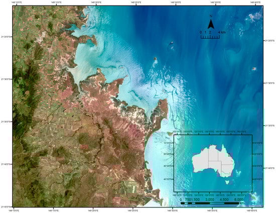
Figure 1.
Study site—Rocky Dam Creek and Cape Palmerston National Park Central Queensland—Sentinel-2B composite image visualised by using the red, green, and blue wavelength bands, captured 31 January 2018 at 00:22:57 provided by United States Geological Survey (USGS).

Table 1.
(IUCN)-listed endangered ecosystems occurring at the study site [20]—Rocky Dam Creek/Cape Palmerston National Park.
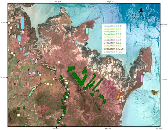
Figure 2.
Sentinel-2B image captured 31 January 2018 with IUCN-endangered ecosystems [20]—Rocky Dam Creek/Cape Palmerston National Park.
Seven broadly recognised mangrove communities occur throughout the region. Within the high rainfall areas of the Central Queensland coast bioregion, estuarine wetlands are about equally dominated by saltpan and samphire flats along the high intertidal area; yellow and orange mangroves (Ceriops tagal and Bruguiera spp.) dominate along the mid-intertidal area; and the stilted mangrove (Rhizophora stylosa) dominates in the lower intertidal area [45]. Twenty-three tree and shrub species of mangroves are present [48]. Landscape elevation ranges from 238 m to sea level; therefore, the study site is not solely within the legislative constraints of the defined coastal area of the Queensland Government (i.e., 5 km from the coastline or where land reaches the height of 10 m; Australian Height Datum [29]).
We used the Sentinel-2B image captured on 31 January 2018 (spatial resolution of 10 m) to overlay the major surface water features of the Plane Creek Basin catchment from the Australian Hydrological Geospatial Fabric (Geofabric) [49] (Figure 3). The map provides a hydrological visualisation of topographically consistent spatial surface water features and stream connectivity. Geospatial stream data are useful for natural resource managers, as streams can be traced upstream and downstream to identify drainage networks and water movement within the catchment area. Here, the map is included to provide information on water connections and hydrology throughout the sub-catchment.
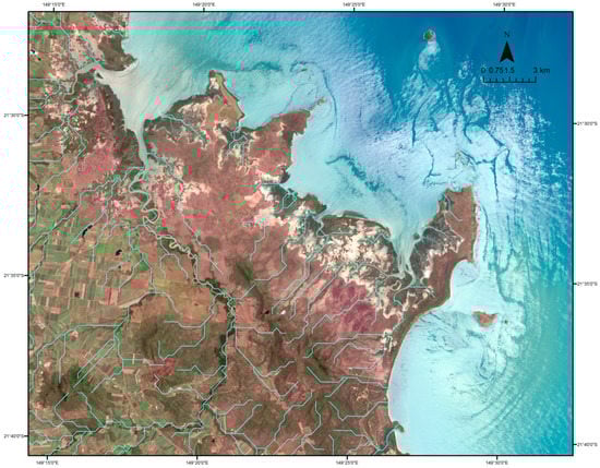
Figure 3.
Sentinel-2B image captured 31 January 2018 overlaid with the Australian Hydrological Geospatial Fabric (Geofabric) [49] showing the drainage networks and hydrological connections of Rocky Dam Creek/Cape Palmerston National Park.
For change detection, we used the Landsat satellite archive images captured in April, August, and September for the years 2004, 2006, 2009, 2013, 2015 and 2017 (Table 2). We acquired images from the United States Geological Survey (USGS) Earth Explorer Landsat Archive at level 1T, (except for 2009) which has systematic radiometric and geometric correction applied to the data by incorporating ground control points and topographic accuracy by utilizing a digital elevation model. The 2009 image was derived from USGS Collection 1 and processed at Tier 1. The 2004, 2006 and 2009 images were taken from the Landsat 5 Thematic Mapper (TM). The 2013, 2015 and 2017 images were taken from Landsat 8 OLI (Operational Land Imager) and TIRS (Thermal Infrared Sensor). Data from Landsat satellites are spatially and geometrically consistent, and they comply with UTM projection [50]. We derived maps from imagery acquired in winter and early spring, as cloud cover inhibits image availability in warmer months [51]. Tidal information corresponding to each image date and time are from the Bureau of Meteorology [52] (Table 2). Medium-resolution satellite imagery is suitable for mapping mangrove and wetland areas on a regional scale [53]. There are two reasons for selecting Landsat imagery: (1) It is acquired at regular intervals, and (2) it is freely available from USGS. We acquired data from two independent sources for use as ground truth data: (1) Queensland Herbarium from 2003, 2006, 2009, 2011, 2013, 2015, and 2017 [54] and (2) Google Earth images from 2005, 2009, 2013, and 2016. Local expert knowledge was included for validation, as this has become an important component of mapping methodology [55].
Table 2.
Image dates and observed sea levels for Hay Point tidal gauge, Central Queensland.
2.2. Image Analysis
All Landsat and Sentinel images were acquired from Earth Explorer and georeferenced to UTM WGS 1984. Data collection included satellite images and ancillary data with local expert knowledge. Prior to the classification of the Landsat images, we stacked the total number of bands in each satellite image by producing a composite. The Mask tool was used to extract the study area and exclude urban coastal regions, the inland region, and the open ocean [56]. Expert knowledge informed the land class designation. Thematic maps produced from the supervised classification were used for change detection in the analyses of thematic change dynamics and the time-series (Figure 4). All image analyses were performed in ArcGIS Version 10.6.1.
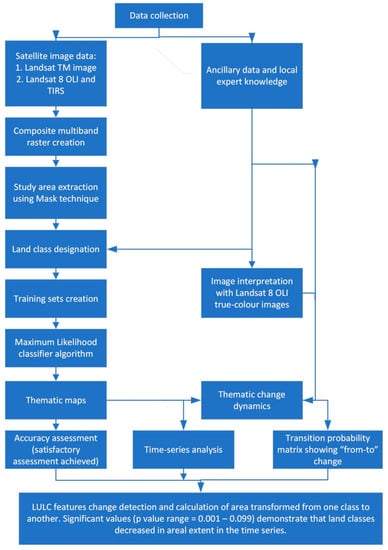
Figure 4.
Methodological workflow used for land use and land cover (LULC) change detection.
2.3. Image Classification
We used a supervised classification method and the ML clustering algorithm with composite images of all Landsat bands. Supervised classification has been the most frequent method by which the remotely sensed data of mangrove areas have been classified, and the ML algorithm has been found to be a robust technique that is capable of repeated refinement and reclassification [14]. With supervised training, it is important that the training area be a homogeneous sample of the respective class but at the same time includes the range of variability for the class [57]. Therefore, more than one training area per class was used. An accurate classification depends on the extent of overlap between class signatures. The ML classifier minimizes the total error in the classification if the estimate of the underlying probability distribution is correct [58]. Based on Bayes’ theorem, the ML algorithm uses a discrimination function to assign pixels to the class with the highest likelihood [59]. Images were classified by using spectral signatures that were obtained from training samples. Training sample polygons represent distinct sample areas of various land cover types to be classified. Distinguishable classes represented by the training samples were examined from the spectral band characteristics [60]. By using the statistical tools in ArcGIS, we determined the samples to be distinguishable by their histograms and distinct scatter-plots [59]. Between 7 and 140 training polygons were generated for each feature class. We classified images into nine information (land) classes: cropping/grazing, oceanic, sand beach, open forest, mangrove forest, estuarine wetland, saltpan, bare mudflat, and saltmarsh grass. Wetland land-use classes include emergent vegetation, riparian vegetation, and riverine and palustrine wetlands (e.g., vegetated swamps) (Table 3).
Table 3.
Land classes used in the classification analysis.
2.4. Accuracy Assessment
We visually compared the spectral classes with reference data derived from high spatial resolution true-colour aerial and satellite images in Google Earth and the Queensland Herbarium at corresponding dates to the Landsat images in order to verify land cover classification accuracy. A stratified random sampling design was appropriate for the accuracy assessment. The random point application in ArcGIS generated approximately 500 unbiased random points, and the validation points were projected onto the classified maps and compared to produce the error matrix. Subsequently, we determined the corresponding change detection thematic map’s user’s accuracies, producer’s accuracies, overall accuracy, and Kappa coefficient [61] (Table 4).
Table 4.
Accuracy assessment of Landsat images captured in 2004 and 2017 at Rocky Dam Creek/Cape Palmerston National Park.
2.5. Change Detection
Change detection procedures estimate that a change in the reflectance of the study area results from a corresponding change in surface cover or surface material [62]. We characterised changes by using a suite of analytics. The first two methods of change detection were post-classification change analysis, and visual interpretation of images and comparison with Google Earth images from similar dates. Using local expert knowledge, we applied the on-screen digitisation of Landsat 2017 true-colour images to show areas of mangroves, saltpan/saltmarsh grass and estuarine wetland that have been altered from 2004 to the oceanic information class in 2017. The third method of change detection was the use of thematic change dynamics by using a remote sensing software tool to portray the dynamics of land cover change that occurred at Rocky Dam Creek/Cape Palmerston National Park. This tool measures the transition dynamics of a land cover class to another class at a given extent. Firstly, an initial state image was input as a time 1 image (2004), and then a final state image was input as time 2 (2017). Only changed areas were taken to visualize the overall dynamics. The output was a transition probability matrix signifying the ‘‘from–to” change that exemplified the past and present state of different land cover classes. The fourth and final method of change detection was a raster-based trend analysis where a time-series stack of thematic maps that was constructed into a 3D array and indexed via row and column was built to get a time-series vector. The occurrence of each class in each pixel across the time-series (i.e., the maximum spatial extent for each class) was used to create the output map. For example, the maximum extent map for open forest would show pixels that contained at least one occurrence of that class across the time-series array. We fitted a linear regression model to the data array with a slope value related to areal cover change per year in the time-series. The trend analysis measured the net change between pixels through the time series data, integrating six raster datasets with the same spatial extent, the output being a spatial map of slope and trend analysis. Information classes were combined to give a broad statistical appraisal of the region’s LULC change dynamics. The map showing slope of the regression line is displayed as ranked data that are representations of the data’s spatial attributes; this was created with the Jenks optimization method, a data clustering method that determines the best arrangement of values into different classes. The method seeks to reduce the variance within classes and maximize the variance between classes. If the values increment in time, they have a positive slope (red area) and, in the case of a decreasing regression line, a negative slope (green area). Temporal relationships were evaluated among the years by using the Pearson’s correlation coefficient r value. Values represent the direction and magnitude of land cover change through the time-series. Post classification change analysis, visual interpretation, and thematic change were quantified by using Erdas Imagine Version 16.5.1 and the Spatial Analyst Toolset in ArcGIS Version 10.6.1. ArcGIS and Python routines were used for the time series analysis.
3. Results
The aim of this research is to quantify how a large, tropical, coastal region with estuarine-dependent fisheries has spatially and temporally changed in a period of 14 years (2004–2017). We used four methods of change detection in the analysis.
3.1. Post Classification Change Analysis
Our post-classification change detection analysis for the Rocky Dam Creek/Cape Palmerston National Park region with images from 2004 and 2017 quantified the amount of change in each land cover type (Figure 5). Information classes with a positive change demonstrated an increase in percentage area, and those with a negative change described a decrease. A positive change was apparent for four of the information classes: cropping/grazing (0.45%, 1329 hectares); oceanic (14%, 13,280 hectares), the large variability for the oceanic class can be explained by the time of day the two images were taken (the 2004 image was captured at low tide and the 2017 image was captured at high tide) (Table 1); saltpan (1.69%, 1565 hectares); and sand flat (0.12%, 126 hectares). A negative change occurred for five of the information classes: open forest (−0.05%, −1851 hectares), mangrove forest (−3.31%, −1147 hectares), estuarine wetland (−3.88%, −1496 hectares), bare mudflat (−5.49%, −2627 hectares), and saltmarsh grass (−3.65%, −1551 hectares) (Table 5). Notably, we found a low occurrence of saltmarsh grass within the park boundary. The overall classification accuracy and Kappa coefficient for 2004, 2006, 2009, 2013 2015, and 2017 land cover maps were 85%, 88%, 88%, 89% 81% and 92%, respectively, which were acceptable accuracy levels (Table 4; Tables S1 and S2 in Supplementary Materials). These values represent the general precision level that can be expected in mapping LULC when using the supervised classification technique.
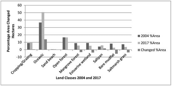
Figure 5.
Land use differences between 2004 and 2017 at Rocky Dam Creek/Cape Palmerston National Park.
Table 5.
Post-classification change statistics for five land use classes: mangrove forest, estuarine wetland, saltmarsh grass, bare mudflat, and saltpan at Rocky Dam Creek/Cape Palmerston National Park.
3.2. Image Interpretation
At the high tide, marine and estuarine waters flood the bays, intertidal flats, and channels of the region which, during wet season events, are diluted to brackish levels in some areas by freshwater flooding and stream flow from the catchment. Freshwater areas are shallow and receive water from stream flow and floodout. Water is otherwise saline throughout and less than 6 m deep. The tidal range is 7 m. The site is a good example of a diverse, hydrologically related aggregation of marine, estuarine, and freshwater wetlands within the Central Queensland Coast bioregion [46]. The Landsat 2017 true-colour composite image exhibits the delineated polygonal outlines of the mangrove (Figure 6), saltpan/saltmarsh grass (Figure 7) and estuarine wetland (Figure 8) classes from the 2004 Landsat image that changed to the oceanic information class. Inundation occurred over a substantial area of three information classes: mangrove forest (87 hectares), saltpan/saltmarsh grass (49 hectares), and estuarine wetland (17 hectares).
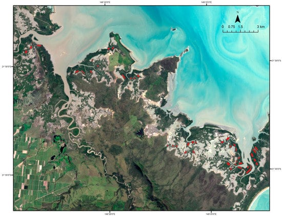
Figure 6.
Landsat 8 Operational Land Imager (OLI) true-colour image captured 27 April 2017 that highlights areas of mangroves that changed to the oceanic information class (shown in red) at Rocky Dam Creek/Cape Palmerston National Park.
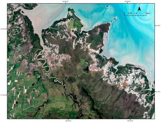
Figure 7.
Landsat 8 OLI true-colour image captured 27 April 2017 that highlights the areas of saltpan/saltmarsh grass that changed to the oceanic information class (shown in orange) at Rocky Dam Creek/Cape Palmerston National Park.
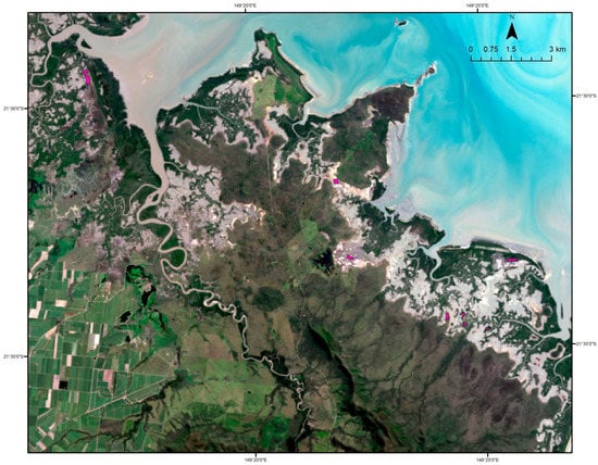
Figure 8.
Landsat 8 OLI true-colour image captured 27 April 2017 that highlights areas of estuarine wetland that changed to the oceanic information class (shown in pink) at Rocky Dam Creek/Cape Palmerston National Park.
3.3. Thematic Change Dynamics
The thematic change summary matrix 2004–2017 shows the number of pixels in each of the nine land classes per zone (Table S3 in the Supplementary Materials) and the net percentage loss of each of the nine land cover classes per zone (Table S4 in the Supplementary Materials). The mangrove land class transitioned to three land classes: (1) open forest (net loss = 5.08%, 597 hectares), (2) estuarine wetland (net loss = 8.51%, 273 hectares), and (3) saltmarsh grass (net loss = 6.26%, 145 hectares). Three information classes transitioned to the cropping/grazing land class over the 14-year time period: the open forest (net loss = 3.3%, 75 hectares), the estuarine wetland (net loss = 4.95%, 552 hectares), and the saltmarsh grass, which deteriorated considerably (net loss = 4.26%, 1001 hectares). A total of 1628 hectares of coastal vegetation transformed into pasture. A proportion of the cropping/grazing land class changed to saltpan (net loss = 5.38%, 192 hectares). The open forest land class claimed a proportion of the estuarine wetland (net loss = 2.16%, 1122 hectares). The bare mudflat information class transitioned to three land classes: (1) saltpan (net loss = 14.44%, 591 hectares), (2) saltmarsh grass (net loss = 2.38%, 66 hectares), and (3) sand flat (net loss = 66.15%, 192 hectares).
3.4. Time Series Analysis
In a spatio–temporal analysis, we used the single explanatory variable of time to explore how the predictor variable, LULC, changed over the landscape 2004–2017. The map of the regression slope shows positive and negative values across the study site (Figure 9). The forested area (mangrove forest and open forest) was the dominant region that occupied the mid-way point in the data range, indicating that this area generally had little inter-annual variability and no decrease on average; this is the yellow area (average r value = 0.24) (Figure 9). A predominantly negative slope of the regression line indicates vegetation thinning and was pronounced in the land classes of cropping/grazing, estuarine wetland, and saltmarsh grass—these are represented by the dark green area (Pearson correlation coefficient r value range = −0.84–0.2) (Figure 10). The total vegetation decline in the cropping/grazing class was 1896 hectares. Strong positive slope values show a high exposure in the system through time but small inter-annual variability. High exposure areas include the saltmarsh grass adjacent to Rocky Dam Creek, saltpan, and bare mudflat land classes across the site extent—these are shown as the orange/red area (Pearson correlation coefficient r value range = 0.37–0.97) (Figure 10). The total change in the combined classes was 9375 hectares. Many areas throughout the study region displayed significant values (p value range = 0.001–0.099), demonstrating that land classes decreased in areal extent in the time series, e.g., the saltmarsh grass south of the saltpan zone, the estuarine wetland south of the saltmarsh grass zone, the bare mudflat in the stream inlets, scattered grazing sites, the open forest at Glendower Point (coastal mid-way point of the site) and the north-east boundary of the park, and the fringing mangroves along the coastline and stream channels.
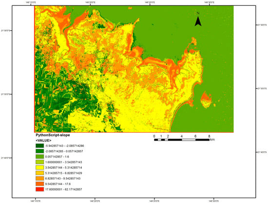
Figure 9.
Map of regression slope that highlights positive and negative values across the study site 2004–2017. High positive slope values show an increase in areal extent through time and are most pronounced in the saltpan and bare mudflat land classes across the site extent (shown in red); high negative slope values show a decrease in areal extent through time and are most pronounced in the land classes: cropping/grazing, estuarine wetland, and saltmarsh grass, as well as the fringing mangroves along the coastline and stream channels (shown in green) at Rocky Dam Creek/Cape Palmerston National Park.
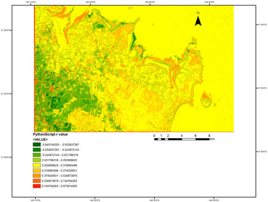
Figure 10.
Map of Pearson correlation coefficient r values across the study site 2004–2017. A strong positive correlation is highlighted in the land classes: saltpan and bare mud flat (shown in red); a strong negative correlation is highlighted in the land classes: cropping/grazing, estuarine wetland, and saltmarsh grass (shown in green). Significant values (p value range = 0.001–0.099) demonstrate that the following land classes decreased in areal extent in the time series: saltmarsh grass, estuarine wetland, bare mudflat in the stream inlets, scattered grazing sites, open forest at Glendower Point (coastal mid-way point of the site) and the north-east boundary of the park, and fringing mangroves along the coastline and stream channels at Rocky Dam Creek/Cape Palmerston National Park.
4. Discussion
4.1. Change Dynamics in Estuarine Ecosystems
Old world tropical mangroves found in the Indo-Pacific, including tropical Australia, possess notable attributes of species diversity, richness, abundance, and succession, and they are therefore considered to be the most dominant and important mangroves globally [63,64]. We examined changes in their vegetation structure and connectivity within a spatially extensive estuarine region of Central Queensland, Australia by using four methods of change detection. This work has relevance to the maintenance of biodiversity and ecological processes because it explores: (1) the distribution of critical wetland habitats in relation to their proximity to threats from human development; (2) temporal change in the distribution and abundance of wetland habitats correlated (spatially) with temporal change in human activities of varying types (fishing, coastal development, agriculture, erosion, and hydrology modification); and (3) interactions that occur at scales larger than a protected area’s boundary that affect the maintenance of biodiversity values.
An analysis of classified maps revealed that gradual ecosystem change occurred across large areas and various habitats. Other studies such as that by Kanniah et al. [65] in the Southern Peninsula, Malaysia, and that of Tran and Fischer [66] in Ca Mao Province, Vietnam, confirm that protected area status does not guarantee the encroachment control of long-term anthropogenic influence, and the downsizing of mangrove communities continues. Competing demands for available resources, especially in coastal provinces, drives change in hydrology and land use outside a protected areas’ administrative boundary, thus affecting ecological processes within such as movement of organisms, water availability, and connectivity functions [31]. Mangroves are well recognised as fragile ecosystems that play an important role in linking marine and terrestrial systems [67]. Nevertheless, it is apparent from our results and most previously published research that mangrove ecosystems are in decline [68,69,70]. The mangroves in our study region are located in the mid and lower intertidal zone and are constrained not by land surface temperature, as in semi-arid regions [71,72], but by air/seawater temperature, freshwater levels, and other geospatial properties. Whilst air/seawater temperature was not measured in this study, other studies have shown a linkage between mangrove deforestation and anthropogenic climate change [73]. The frequency and intensity of cyclones and storms has increased as a consequence of greater sea-surface temperature, with further escalation predicted [74,75]. The Landsat 2017 image was captured in April immediately following the impact of a severe tropical cyclone [16]. We suggest that the mangrove decline in our study (1147 hectares) was a result of change in sediment profiles, defoliation, and inundation from a coastal cyclone [74,76]. Furthermore, because effects outside the boundary of a protected area manifest themselves within that boundary, alterations in hydrology for pasture and direct trampling may be linked to the decline in mangroves, saltmarsh grass, and estuarine wetlands. Similarly, Al-Hamdan et al. [77], by using Landsat satellite data in Tanzania during the period of 2000–2010, found a net deforestation of mangroves with a net agriculture expansion. Our result for mangrove transition (1015 hectares) from the thematic change analysis is comparable to Chen et al. [78], who observed the transition of mangroves to other land uses during the period of 1985–2013 in the Honduras.
River and stream flow regulation is pervasive in Australia. River regulation affects riverine vegetation by fundamentally altering the flow regime, thus changing the hydrology and flow across a range of different spatial and temporal scales [79]. Though there is recognition by government agencies of the alienation of flow-dependent ecosystems that are attributed to anthropogenic barriers [22], regulating structures such as culverts, pipes, road crossings, weirs, and ponded pasture still potentially cause connectivity disruption in our study region [80]. Further, the inclusion of regulating structures interrupts stream flow regimes, floodplain–wetland connections, biotic responses, channel formation, and sediment transfer [81]. The fragmentation of riverine vegetation with corresponding environmental degradation from flow regulation has been observed with Landsat imagery in other studies, such as those by Das and Pal [82] in India and Antwi et al. [83] in Ghana. We suggest that the reduction in estuarine wetland in our study (1496 hectares) including endangered ecosystems, in combination with a significant declining trend in vegetation extent (thinning) (Table 1, Figure 2), was primarily due to the alteration of natural flow regimes through stream regulation, which affected the processes that sustain riparian vegetation communities.
Saltmarsh grass is recognized as providing climate benefits through carbon sequestration as well as other ecosystem benefits, e.g., storm surge erosion protection and ontogenetic habitat for fisheries species [9,84]. Tropical saltmarsh grass is poorly represented in protected areas and crudely acknowledged for its ecosystem services when confronted with alternative land uses. In a recent review, Wegscheidl et al. [85] identified a lack of quantitative information needed to substantiate the value of Australia’s saltmarshes, both locally and regionally. Likewise, we found a low occurrence of saltmarsh grass in Cape Palmerston National park, and there was an apparent decreasing trend in the vegetation extent (thinning) of saltmarsh grass throughout the study site. Saltpan and bare mudflat areas exhibited inconsistency across the study site. There were high levels of bare mudflat accretion in the main channels and areas of coastline; however, stream inlets and drainage networks showed inter-annual variability (long-term trend increases and decreases) due to tidal fluctuations and a decrease through time. Similar to those reported by previous studies in tropical regions [86], our results suggest that the saltmarsh–mudflat system in the landward region of the Cape Palmerston National Park shows instability and is degrading over time, possibly due to climatic factors such as recent cyclonic activity, sea level variability, and prolonged inundation.
The need for scientifically-based regional-scale land use planning around protected areas is integral in human-dominated landscapes to balance conservation goals with livelihood needs for crops, pasture, and other ecosystem services [31]. The decline in wetland ecosystems in our study could be attributed to both direct and indirect effects. Direct effects could include altered vegetation composition and structure from trampling by grazing animals and the modification of ground morphology. An indirect effect could include the draining and hydrological disturbances that convert wetlands to agricultural and grazing land, resulting in tidal disruption and vegetation fragmentation. Across the sub-catchment, the cumulative area of open forest, estuarine wetland, and saltmarsh grass (1628 hectares) was converted to pasture. Riverine landscapes are highly valued in Australia for grazing and are often preferred by livestock because of their vegetation, shade, and water [87]. Though the Sarina Inlet–Ince Bay Aggregation is a designated important wetland under Australian federal biodiversity conservation policy [46], implementation is lacking [88]. The land classes that are open forest and estuarine wetland transition to cropping/grazing is a similar result to that obtained by Haque and Basak [37], who found that forested land transitioned to either shallow water or settlement in Bangladesh during 1980–2010. The result by Toure et al. [89] in Senegal with Landsat imagery and ML classification highlighted the unexpected transition of agriculture to saltpan, as was the case for areas of cropping/grazing in our study (192 hectares).
The significant declining trend observed for open forest, fringing mangroves, estuarine wetlands, and vegetation levels in scattered grazing sites was inconsistent across the study area. This inconsistency illustrates how multiple forms of change can co-occur within relatively close proximity. We suggest that the decline in shoreline vegetation cover was the direct result of a severe tropical cyclone that impacted the coast in March 2017, and we also suggest that grazing-induced, ubiquitous vegetation degradation contributed to and will continue to exacerbate the loss of resilience in these systems.
4.2. Comparison with SLATS
The SLATS program was initiated by the Queensland Government to provide factual information on land cover and trends in land clearing, tree growth, and regrowth on public and private lands [90]. The SLATS data are based on the supervised classification of multiple Landsat satellite images and digital terrain models at a resolution of approximately 30 m, with maps on woody vegetation clearing (and replacement land cover) that are the result of the anthropogenic removal of vegetation [91]. SLATS has clear differences with our study in that SLATS does not include any vegetation loss caused by natural tree death or natural disasters (e.g., cyclones) when calculating woody vegetation clearing rates. Further, SLATS applies radiometric standardisation to the Landsat images. Finally, topographic corrections are used to increase accuracy in areas of high slope [92]. However, as our study area is generally of low, flat elevation, we deemed the correction unnecessary. An inspection of SLATS maps from 2004 to 2017 in ArcGIS displayed similarities with our results with many sites cleared of woody vegetation and converted to pasture, particularly along the boundary of the national park, in the north-east, north-west, south, and central areas. According to SLATS, the total converted vegetation in the Plane Creek catchment is 3536 hectares, and, by digitizing the Rocky Dam Creek sub-catchment pasture polygons in ArcGIS, we found a total of 1100 hectares. Though the total SLATS pasture profile is smaller than our results for the thematic change (1628 hectares) and time series (1896 hectares), our results nevertheless reflect a variable but significant impact on the coastal region that was likely caused by an intense climatic event.
4.3. Limitations of the Study
Remote sensing data and tools are fundamental methods for measuring LULC, but there are critical drawbacks in the change detection of wetlands. The first drawback is that classification errors from the individual-date images can affect the final change detection accuracy, and, although ground-truth data engender the development of accurate LULC classification and accuracy assessments, errors can still occur [93]. Foody [94] argued that accuracy values cannot be appropriately interpreted by readers or users unless a detailed account of the approach to accuracy assessment is provided. The lack of robust validation could have serious implications for some users and may lessen their confidence in remote sensing as a source of land cover data. Therefore, the validation methods that detail the user’s and producer’s accuracies of change with Kappa coefficient and which include the confusion matrix for the 2004 and 2017 images (Table 4) have been given to allow for replication. The second drawback is that during high tides, there can be a sharp decline in the spectral reflectance of mangroves, especially in the NIR and SWIR regions [95,96]. Our study used a combined binary change detection and time series analysis approach, illustrating that it is beneficial to use multiple images in change detection research since apparent changes between any two images could be due to irrelevant causes such as tide, sea surface state, and water constituents. The third drawback is that, ideally, change detection requires precise image alignment, which is difficult to achieve, and the fourth drawback is that post classification comparison-based binary approaches that are used for hard classifications, i.e., comparatively broad scale classifications, may not detect subtle transformations in land cover modification in which the land cover type may have been altered but not changed (e.g., a thinned forest or saltmarsh degradation), ensuing an inappropriate representation [97].
4.4. Implications for the Conservation of Estuarine Ecosystems
Quantifying the level of coastal wetland fragmentation and landscape connectivity is an essential component of contemporary strategies that are aimed at biodiversity conservation and fishery sustainability [98]. The results presented here are noteworthy from two viewpoints. The first is nationally—in Australia, there is no nationally consistent approach to quantify the area of mangrove or saltmarshes, and historical benchmarks are scarce [99]. Our results inform the Australian inventory of spatio–temporal distribution, as they show important changes in the representation of coastal vegetation classes, particularly mangroves and saltmarsh grasses, in the tropical catchments of the Eastern seaboard. The second viewpoint is regionally—natural resource management is hampered by complex management arrangements that provide challenges to achieving environmental sustainability and are additional to increasing pressures from natural and anthropogenic forces [100]. Our findings raise concerns that lands surrounding the Cape Palmerston National Park are under threat, and, because interactions occur at scales larger than a protected areas’ boundary, repercussions arise for the environmental stability of the entire region. Watson et al. [101] argue that the occurrence of threatened species is widespread outside protected areas, and plants are one of the most poorly represented taxonomic groups. Furthermore, protected areas are not exempt from anthropogenic impacts; for example, Jones et al. [102] identified an increase of human pressure of 1.5% on IUCN listed protected areas categories I and II between 1993 and 2009. Particularly evident in our study was the decline of estuarine wetlands, which include endangered ecosystems: the broad leaf tea-tree Malaleuca viridiflora and semi-evergreen microphyll vine thicket-to-vine forest [103] (Figure 2).
There is a need for a more comprehensive understanding of the ecosystem value assigned to Australia’s coastal landscapes. This information is a high priority and needed to support evidence-based decision-making and conservation actions that attribute socio–economic value, warranting ecosystem protection and repair [85]. For example, the Australian Government listed subtropical and temperate coastal saltmarsh as a vulnerable ecological community under the Environment Protection and Biodiversity Conservation Act 1999 (EPBC) in 2013 [104]. Carbon sequestration pathways designate saltmarshes (and other coastal wetlands) as disproportionality valuable in sequestering carbon dioxide compared to terrestrial ecosystems [105]. Therefore, it is an opportune time to apply protection to these communities. We propose that the vulnerable listing be extended to tropical saltmarsh regions. The 1998–2003 historical occurrence of mangrove dieback in local estuaries, which affected >30 km2 of remnant mangrove cover [106,107], failed to conclusively identify the causative agent (agricultural herbicides and flooding were implicated in the event). However, recent northern Australian mangrove dieback has been linked to climate change as the most likely cause [108]. The declining trend in fringing mangroves found in our study is concomitant to a loss of ecosystem services that are provided by the coastal habitat–fishery linkage, as the service value of mangroves has been observed to be higher at the seaward edge [109]. Notwithstanding the Australian government’s efforts to provide protection to Great Barrier Reef catchments [16], ecosystem degradation is ongoing.
Two key factors determine the extent to which coastal habitats can recover and the associated fauna rejuvenate from a major acute (pulse-like) disturbance such as a cyclone: (1) the time window until the next major acute disturbance [110] and (2) the extent and intensity of chronic (press-like) disturbances, such as disruption in sediment/water profiles [74] and elevated mean seawater temperatures suppressing recovery rates [64] during that window. Predictions that tropical cyclones will increase in frequency and intensity in Australia in the coming decades [111] have been accompanied by projections of an escalation in storm surges and extreme sea-levels under future climate change [112]. Improving the resilience of Great Barrier Reef coastal ecosystems requires active landscape protection and restoration approaches to maintain as many biodiversity and ecosystem functions as possible [113].
5. Conclusions
In this paper, we have used a stratification approach to examine different types of change by analysing land cover types. Ancillary data and local expert knowledge were necessary to expose long-term trends and formulate explanations in a region that surrounds and includes a national park that has, until now, been largely devoid of significant direct anthropogenic impact. Whereas the reasons for such changes could generally be explained with detailed field-based data sets, such information does not exist at the requisite spatial and temporal scales. Remote sensing datasets, e.g., Landsat imagery, provided the only feasible method to enumerate the trends in LULC in the spatially extensive study area. Areal reduction in threatened and endangered ecosystems (e.g., mangroves and estuarine wetlands) occurred within Cape Palmerston National Park and its surroundings. We found a decreasing trend in the vegetation extent of estuarine wetlands, saltmarsh grass, and grazing areas. Significant declining values were observed in open forest, fringing mangroves, estuarine wetlands, and saltmarsh grass, albeit on localized scales, with a mosaic of ensemble change across the study site. The occurrence of a severe tropical cyclone immediately preceding capture of the 2017 Landsat image was likely the main agent in the declining trend for shoreline and stream vegetation. Long-term grazing pressure contributed to vegetation degradation and loss of resilience on a landscape scale. SLATS maps confirm that many sites in the sub-catchment were cleared of woody vegetation and converted to pasture during our time period. To maintain ecosystem services and encourage habitat–fishery linkages, effective monitoring action is crucial to understand recovery and set in place adaptive management approaches. Historical occurrence of mangrove dieback in the region, coupled with the recent calls for the increased monitoring of northern Australian mangrove ecosystems due to dieback connections to climate change, could be extended to Great Barrier Reef catchments. Future studies by the authors will create virtual constellation synergies by integrating optical land imaging systems with similar characteristics, e.g., Landsat and Sentinel-2, firstly to assess post-cyclone recovery and secondly to explore ecosystem variability forced by climate controls in Great Barrier Reef catchments. Our research contributes to the body of knowledge on coastal ecosystem dynamics to enable planning to achieve more effective conservation outcomes.
Supplementary Materials
The following are available online at https://www.mdpi.com/2072-4292/12/1/197/s1, Table S1: Accuracy assessment of Landsat image captured in 2004, Rocky Dam Creek/Cape Palmerston National Park, Table S2: Accuracy assessment of Landsat image captured in 2017, Rocky Dam Creek/Cape Palmerston National Park, Table S3: Thematic Change Summary Matrix 2004–2017 with number of pixels in each land class per zone Rocky Dam Creek/Cape Palmerston National Park, Table S4: Thematic Change Summary Matrix 2004–2017 with percentage of land classes occurring in each zone Rocky Dam Creek/Cape Palmerston National Park.
Author Contributions
Conceptualization, S.P.; formal analysis, D.C.; methodology, D.C.; resources, H.P.; supervision, S.P. and H.P.; writing—original draft, D.C.; writing—review and editing, S.P. and H.P. All authors have read and agreed to the published version of the manuscript.
Funding
This research received no external funding.
Acknowledgments
Technical support was gratefully received from Steve Bryant of Mackay State High School (Mackay, QLD 4740, Australia).
Conflicts of Interest
The authors declare no conflict of interest.
References
- Allgeier, J.E.; Layman, C.A.; Mumby, P.J.; Rosemond, A.D. Biogeochemical implications of biodiversity and community structure across multiple coastal ecosystems. Ecol. Monogr. 2015, 85, 117–132. [Google Scholar] [CrossRef]
- Cloern, J.E.; Abreu, P.C.; Carstensen, J.; Chauvaud, L.; Elmgren, R.; Grall, J.; Greening, H.; Johansson, J.O.; Kahru, M.; Sherwood, E.T.; et al. Human activities and climate variability drive fast-paced change across the world’s estuarine-coastal ecosystems. Glob. Chang. Biol. 2016, 22, 513–529. [Google Scholar] [CrossRef] [PubMed]
- Costanza, R.; de Groot, R.; Sutton, P.; van der Ploeg, S.; Anderson, S.J.; Kubiszewski, I.; Farber, S.; Turner, R.K. Changes in the global value of ecosystem services. Glob. Environ. Chang. 2014, 26, 152–158. [Google Scholar] [CrossRef]
- Al-Nasrawi, A.; Hopley, C.; Hamylton, S.; Jones, B. A spatio-temporal assessment of landcover and coastal changes at Wandandian Delta System, Southeastern Australia. J. Mar. Sci. Eng. 2017, 5, 55. [Google Scholar] [CrossRef]
- Ballanti, L.; Byrd, K.; Woo, I.; Ellings, C. Remote sensing for wetland mapping and historical change detection at the Nisqually River Delta. Sustainability 2017, 9, 191. [Google Scholar] [CrossRef]
- Li, D.; Lu, D.; Wu, M.; Shao, X.; Wei, J. Examining land cover and greenness dynamics in Hangzhou Bay in 1985–2016 using Landsat time-series data. Remote Sens. 2017, 10, 32. [Google Scholar] [CrossRef]
- Schmidt, M.; Lucas, R.; Bunting, P.; Verbesselt, J.; Armston, J. Multi-resolution time series imagery for forest disturbance and regrowth monitoring in Queensland, Australia. Remote Sens. Environ. 2015, 158, 156–168. [Google Scholar] [CrossRef]
- Reuter, K.E.; Juhn, D.; Grantham, H.S. Integrated land-sea management: Recommendations for planning, implementation and management. Environ. Conserv. 2016, 43, 181–198. [Google Scholar] [CrossRef]
- Sheaves, M.; Barnett, A.; Bradley, M.; Abrantes, K.G.; Brians, M.; James Cook University. Life History Specific Habitat Utilisation of Tropical Fisheries Species; FRDC Project No 2013-046; James Cook University: Townsville, Australia, 2016. [Google Scholar]
- Peirson, W.; Davey, E.; Jones, A.; Hadwen, W.; Bishop, K.; Beger, M.; Capon, S.; Fairweather, P.; Creese, B.; Smith, T.F.; et al. Opportunistic management of estuaries under climate change: A new adaptive decision-making framework and its practical application. J. Environ. Manag. 2015, 163, 214–223. [Google Scholar] [CrossRef]
- Creighton, C.; Boon, P.I.; Brookes, J.D.; Sheaves, M. Repairing Australia’s estuaries for improved fisheries production—What benefits, at what cost? Mar. Freshw. Res. 2015, 66, 493–507. [Google Scholar] [CrossRef]
- Barbier, E.B.; Hacker, S.D.; Kennedy, C.; Koch, E.W.; Stier, A.C.; Silliman, B.C. The value of estuarine & coastal ecosystem services. Ecol. Monogr. 2011, 81, 169–193. [Google Scholar]
- van der Stocken, T.; Carroll, D.; Menemenlis, D.; Simard, M.; Koedam, N. Global-scale dispersal and connectivity in mangroves. Proc. Natl. Acad. Sci. USA 2019, 116, 915–922. [Google Scholar] [CrossRef] [PubMed]
- Green, K.; Congalton, R.; Tukman, M. Imagery and GIS: Best Practices for Extracting Information from Imagery; Esri Press: Redlands, CA, USA, 2017. [Google Scholar]
- Ferro-Azcona, H.; Espinoza-Tenorio, A.; Calderón-Contreras, R.; Ramenzoni, V.C.; Gómez País, M.; Mesa-Jurado, M.A. Adaptive capacity and social-ecological resilience of coastal areas: A systematic review. Ocean Coast. Manag. 2019, 173, 36–51. [Google Scholar] [CrossRef]
- Commonwealth of Australia. Reef 2050 Long-Term Sustainability Plan-July 2018; Department of the Environment, Commonwealth of Australia: Canberra, Australia, 2018; pp. 9–13, 92–93. [Google Scholar]
- Fang, X.; Hou, X.; Li, X.; Hou, W.; Nakaoka, M.; Yu, X. Ecological connectivity between land and sea: A review. Ecol. Res. 2018, 33, 51–61. [Google Scholar] [CrossRef]
- Schaffelke, B.; Mellors, J.; Duke, N.C. Water quality in the Great Barrier Reef region: Responses of mangrove, seagrass and macroalgal communities. Mar. Pollut. Bull. 2005, 51, 279–296. [Google Scholar] [CrossRef] [PubMed]
- Spalding, M.D.; Ruffo, S.; Lacambra, C.; Meliane, I.; Hale, L.Z.; Shepard, C.C.; Beck, M.W. The role of ecosystems in coastal protection: Adapting to climate change and coastal hazards. Ocean Coast. Manag. 2014, 90, 50–57. [Google Scholar] [CrossRef]
- Queensland Herbarium. Regional Ecosystem Description Database (REDD) Version 11 (December 2018). Available online: https://apps.des.qld.gov.au/regional-ecosystems/ (accessed on 1 March 2019).
- Reef Catchments Limited. Natural Resource Management Plan, Mackay Whitsunday Isaac 2014–2024; Reef Catchments Limited: Mackay, Australia, 2014; pp. 1–29, 60–87. [Google Scholar]
- Moore, M. Mackay Whitsunday Fish Barrier Prioritisation Report; Catchment Solutions: Mackay, Australia, 2015. [Google Scholar]
- Duke, N.C.; Roelfsema, C.; Tracey, D.; Godson, L. Preliminary Investigation into the Dieback of Mangroves in the Mackay Region: Initial Assessment and Primary Causes; University of Queensland: Brisbane, Australia, 2001. [Google Scholar]
- Sheaves, M.; Brookes, J.; Coles, R.; Freckelton, M.; Groves, P.; Johnston, R.; Winberg, P. Repair and revitalisation of Australia’s tropical estuaries and coastal wetlands: Opportunities and constraints for the reinstatement of lost function and productivity. Mar. Policy 2014, 47, 23–38. [Google Scholar] [CrossRef]
- Olds, A.D.; Connolly, R.M.; Pitt, K.A.; Pittman, S.J.; Maxwell, P.S.; Huijbers, C.M.; Moore, B.R.; Albert, S.; Rissik, D.; Babcock, R.C.; et al. Quantifying the conservation value of seascape connectivity: A global synthesis. Glob. Ecol. Biogeogr. 2015, 25, 3–15. [Google Scholar] [CrossRef]
- Carrasquilla-Henao, M.; Juanes, F. Mangroves enhance local fisheries catches: A global meta-analysis. Fish Fish. 2016, 1–15. [Google Scholar] [CrossRef]
- Manson, F.J.; Loneragan, N.R.; Skilleter, G.A.; Phinn, S.R. An evaluation of the evidence for linkages between mangroves and fisheries. Oceanogr. Mar. Biol. 2005, 43, 485–515. [Google Scholar]
- Adam, P. Salt Marsh Restoration. In Coastal Wetlands, 2nd ed.; Perillo, G.M.E., Wolanski, E., Eds.; Elsevier: Amsterdam, The Netherlands, 2019; pp. 817–861. [Google Scholar] [CrossRef]
- Great Barrier Reef Marine Park Authority. Great Barrier Reef Region Strategic Assessment: Strategic Assessment Report; GBRMPA: Townsville, Australia, 2014; pp. 197–281, 325–327, 441–476. [Google Scholar]
- Creighton, C. Revitalising Australia’s Estuaries; Final Report—2012-036-DLD; Fisheries Research and Development Corporation: Canberra, Australia, 2013; pp. 1–38, 145–165. [Google Scholar]
- DeFries, R.; Karanth, K.K.; Pareeth, S. Interactions between protected areas and their surroundings in human-dominated tropical landscapes. Biol. Conserv. 2010, 143, 2870–2880. [Google Scholar] [CrossRef]
- Jones, D.A.; Hansen, A.J.; Bly, K.; Doherty, K.; Verschuyl, J.P.; Paugh, J.I.; Carle, R.; Story, S.J. Monitoring land use and cover around parks: A conceptual approach. Remote Sens. Environ. 2009, 113, 1346–1356. [Google Scholar] [CrossRef]
- Macintosh, A. The National Greenhouse Accounts & Land Clearing: Do the Numbers Stack Up? Research Paper No. 38; Australia Institute: Canberra, Australia, 2007. [Google Scholar]
- Singh, A. Digital change detection techniques using remotely-sensed data. Int. J. Remote Sens. 1989, 10, 989–1003. [Google Scholar] [CrossRef]
- Lu, D.; Li, G.; Moran, E. Current situation and needs of change detection techniques. Int. J. Image Data Fusion 2014, 5, 13–38. [Google Scholar] [CrossRef]
- Gómez, C.; White, J.C.; Wulder, M.A. Optical remotely sensed time series data for land cover classification: A review. ISPRS J. Photogramm. Remote Sens. 2016, 116, 55–72. [Google Scholar] [CrossRef]
- Haque, M.I.; Basak, R. Land cover change detection using GIS and remote sensing techniques: A spatio-temporal study on Tanguar Haor, Sunamganj, Bangladesh. Egypt. J. Rem. Sens. Space Sci. 2017, 20, 251–263. [Google Scholar] [CrossRef]
- Jones, T.; Glass, L.; Gandhi, S.; Ravaoarinorotsihoarana, L.; Carro, A.; Benson, L.; Ratsimba, H.; Giri, C.; Randriamanatena, D.; Cripps, G. Madagascar’s mangroves: Quantifying nation-wide and ecosystem specific dynamics, and detailed contemporary mapping of distinct ecosystems. Remote Sens. 2016, 8, 106. [Google Scholar] [CrossRef]
- Richards, J.A.; Jia, X. Remote Sensing Digital Image Analysis: An Introduction, 4th ed.; Springer: Berlin/Heidelberg, Germany, 2006; pp. 1–78, 137–160, 193–238, 295–328, 389–413, 423–428. [Google Scholar]
- Barik, K.K.; Mitra, D.; Annadurai, R.; Tripathy, J.K.; Nanda, S. Geospatial analysis of coastal environment: A case study on Bhitarkanika mangroves, East coast of India. Indian J. Geo-Mar. Sci. 2016, 45, 492–498. [Google Scholar]
- Xu, C.; Pu, L.; Zhu, M.; Li, J.; Chen, X.; Wang, X.; Xie, X. Ecological security and ecosystem services in response to land use change in the coastal area of Jiangsu, China. Sustainability 2016, 8, 816. [Google Scholar] [CrossRef]
- Folkers, A.; Rohde, K.; Delaney, K.; Flett, I. Mackay Whitsunday Water Quality Improvement Plan 2014–2021; Reef Catchments (Mackay Whitsunday Isaac) Limited: Mackay, Australia, 2014; pp. 11–33, 43–63, 107. [Google Scholar]
- Pascoe, S.; Innes, J.; Tobin, R.; Stoeckle, N.; Paredes, S.; Dauth, K. Beyond GVP: The Value of Inshore Commercial Fisheries to Fishers and Consumers in Regional Communities on Queensland’s East Coast; FRDC Project No 2013-301; Fisheries Research and Development Corporation: Canberra, Australia, 2016; pp. 1–79. [Google Scholar]
- Webley, J.; McInnes, K.; Teixeira, D.; Lawson, A.; Quinn, R. Statewide Recreational Fishing Survey 2013-14; Department of Agriculture and Fisheries: Brisbane, Australia, 2015; pp. 82–83. [Google Scholar]
- Reef Catchments. State of the Region Report, Mackay Whitsunday Isaac; Reef Catchments: Mackay, Australia, 2013. [Google Scholar]
- Department of the Environment. Directory of Important Wetlands in Australia, Sarina Inlet-Ince Bay Aggregation-QLD053. Available online: https://www.environment.gov.au/cgi-bin/wetlands/report.pl (accessed on 1 March 2019).
- IUCN. World Database on Protected Areas Cape Palmerston-Rocky Dam in Australia. Available online: https://protectedplanet.net/23846 (accessed on 1 March 2019).
- Duke, N.C.; Larkum, A.W.D. Mangroves and Seagrasses. In The Great Barrier Reef: Biology, Environment and Management; Hutchings, P., Kingsford, M., Eds.; CSIRO Publishing: Collingwood, Australia, 2008; pp. 1–18. [Google Scholar]
- Bureau of Meteorology. Australian Hydrological Geospatial Fabric (Geofabric) Product Guide Version 3.0; Bureau of Meteorology: Canberra, Australia, 2015. [Google Scholar]
- USGS. Landsat Collection 1 Level 1 Product Definition Version 1.0; United States Geological Survey: South Dakota, USA, 2017. [Google Scholar]
- Lyons, M.B.; Phinn, S.R.; Roelfsema, C.M. Long term land cover and seagrass mapping using Landsat and object-based image analysis from 1972 to 2010 in the coastal environment of South East Queensland, Australia. ISPRS J. Photogramm. Remote Sens. 2012, 71, 34–46. [Google Scholar] [CrossRef]
- Bureau of Meteorology. Tide Predictions for Australia, South Pacific and Antarctica. Available online: http://www.bom.gov.au/australia/tides/ (accessed on 1 March 2019).
- Kuenzer, C.; Bluemel, A.; Gebhardt, S.; Quoc, T.V.; Dech, S. Remote sensing of mangrove ecosystems: A review. Remote Sens. 2011, 3, 878–928. [Google Scholar] [CrossRef]
- Neldner, V.J.; Niehus, R.E.; Wilson, B.A.; McDonald, W.J.F.; Ford, A.J.; Accad, A. The Vegetation of Queensland: Descriptions of Broad Vegetation Groups. Version 4.0; Queensland Herbarium, Department of Environment and Science: Brisbane, Australia, 2019. [Google Scholar]
- Australian Bureau of Agricultural and Resource Economics and Sciences. Guidelines for Land Use Mapping in Australia: Principles, Procedures and Definitions, 4th ed.; Australian Bureau of Agricultural and Resource Economics and Sciences: Canberra, Australia, 2011. [Google Scholar]
- Long, J.B.; Giri, C. Mapping the Philippines’ mangrove forests using Landsat imagery. Sensors 2011, 11, 2972–2981. [Google Scholar] [CrossRef] [PubMed]
- Soto-Berelov, M.; Hislop, S. Approaches Used for Pixel Based Time Series Analysis of Landsat Data: Literature Review; RMIT University: Melbourne, Australia, 2016. [Google Scholar]
- Vogelmann, J.E.; Gallant, A.L.; Shi, H.; Zhu, Z. Perspectives on monitoring gradual change across the continuity of Landsat sensors using time-series data. Remote Sens. Environ. 2016, 185, 258–270. [Google Scholar] [CrossRef]
- Abdul Aziz, A.; Phinn, S.; Dargusch, P.; Omar, H.; Arjasakusuma, S. Assessing the potential applications of Landsat image archive in the ecological monitoring and management of a production mangrove forest in Malaysia. Wetl. Ecol. Manag. 2015, 23, 1049–1066. [Google Scholar] [CrossRef]
- Nguyen, H.-H.; McAlpine, C.; Pullar, D.; Johansen, K.; Duke, N.C. The relationship of spatial–temporal changes in fringe mangrove extent and adjacent land-use: Case study of Kien Giang coast, Vietnam. Ocean Coast. Manag. 2013, 76, 12–22. [Google Scholar] [CrossRef]
- Jensen, J.R. Introductory Digital Image Processing: A Remote Sensing Perspective, 4th ed.; Pearson Education: Glenview, IL, USA, 2015; pp. 501–582. [Google Scholar]
- El-Hattab, M.M. Applying post classification change detection technique to monitor an Egyptian coastal zone (Abu Qir Bay). Egypt. J. Rem. Sens. Space Sci. 2016, 19, 23–36. [Google Scholar] [CrossRef]
- Ajai; Bahuguna, A.; Chauhan, H.B.; Sen Sarma, K.; Bhattacharya, S.; Ashutosh, S.; Pandey, C.N.; Thangaradjou, T.; Gnanppazham, L.; Selvam, V.; et al. Mangrove inventory of India at community level. Natl. Acad. Sci. Lett. 2013, 36, 67–77. [Google Scholar] [CrossRef]
- Saintilan, N.; Rogers, K.; Kelleway, J.J.; Ens, E.; Sloane, D.R. Climate change impacts on the coastal wetlands of Australia. Wetlands 2018, 38, 1–10. [Google Scholar] [CrossRef]
- Kanniah, K.; Sheikhi, A.; Cracknell, A.; Goh, H.; Tan, K.; Ho, C.; Rasli, F. Satellite images for monitoring mangrove cover changes in a fast growing economic region in Southern Peninsular Malaysia. Remote Sens. 2015, 7, 14360–14385. [Google Scholar] [CrossRef]
- Tran, L.X.; Fischer, A. Spatiotemporal changes and fragmentation of mangroves and its effects on fish diversity in Ca Mau Province (Vietnam). J. Coast Conserv. 2017, 21, 355–368. [Google Scholar] [CrossRef]
- Olds, A.D.; Albert, S.; Maxwell, P.S.; Pitt, K.A.; Connolly, R.M. Mangrove-reef connectivity promotes the effectiveness of marine reserves across the western Pacific. Glob. Ecol. Biogeogr. 2013, 22, 1040–1049. [Google Scholar] [CrossRef]
- Eyoh, A.; Ebom, O. Spatio-temporal analysis of land use/land cover change trend of Akwa Ibom State, Nigeria from 1986–2016 using remote sensing and GIS. Intl. J. Sci. Res. 2015, 5, 1805–1809. [Google Scholar] [CrossRef]
- Jones, T.; Ratsimba, H.; Ravaoarinorotsihoarana, L.; Glass, L.; Benson, L.; Teoh, M.; Carro, A.; Cripps, G.; Giri, C.; Gandhi, S.; et al. The dynamics, ecological variability and estimated carbon stocks of mangroves in Mahajamba Bay, Madagascar. J. Mar. Sci. Eng. 2015, 3, 793–820. [Google Scholar] [CrossRef]
- Richards, D.R.; Friess, D.A. Rates and drivers of mangrove deforestation in Southeast Asia, 2000–2012. Proc. Natl. Acad. Sci. USA 2016, 113, 344–349. [Google Scholar] [CrossRef] [PubMed]
- Duke, N.C.; Kovacs, J.M.; Griffiths, A.D.; Preece, L.; Hill, D.J.E.; van Oosterzee, P.; Mackenzie, J.; Morning, H.S.; Burrows, D. Large-scale dieback of mangroves in Australia. Mar. Freshw. Res. 2017, 68, 1816–1829. [Google Scholar] [CrossRef]
- Hickey, S.M.; Phinn, S.R.; Callow, N.J.; Van Niel, K.P.; Hansen, J.E.; Duarte, C.M. Is climate change shifting the poleward limit of mangroves? Estuaies Coasts 2017, 40, 1215–1226. [Google Scholar] [CrossRef]
- Rodriguez, W.; Feller, I.C.; Cavanaugh, K.C. Spatio-temporal changes of a mangrove–saltmarsh ecotone in the northeastern coast of Florida, USA. Glob. Ecol. Conserv. 2016, 7, 245–261. [Google Scholar] [CrossRef]
- Asbridge, A.; Lucas, R.; Accad, A.; Dowling, R. Mangrove response to environmental changes predicted under varying climates: Case studies from Australia. Curr. For. Rep. 2015, 1, 178–194. [Google Scholar] [CrossRef]
- Hoque, M.A.-A.; Phinn, S.; Roelfsema, C. A systematic review of tropical cyclone disaster management research using remote sensing and spatial analysis. Ocean Coast. Manag. 2017, 146, 109–120. [Google Scholar] [CrossRef]
- McInnes, K. Wet Tropics Cluster Report, Climate Change in Australia: Projections for Australia’s Natural Resource Management Regions; CSIRO and Bureau of Meteorology: Canberra, Australia, 2015. [Google Scholar]
- Al-Hamdan, M.Z.; Oduor, P.; Flores, A.I.; Kotikot, S.M.; Mugo, R.; Ababu, J.; Farah, H. Evaluating land cover changes in Eastern and Southern Africa from 2000 to 2010 using validated Landsat and MODIS data. Int. J. Appl. Earth Obs. Geoinf. 2017, 62, 8–26. [Google Scholar] [CrossRef]
- Chen, C.-F.; Son, N.-T.; Chang, N.-B.; Chen, C.-R.; Chang, L.-Y.; Valdez, M.; Centeno, G.; Thompson, C.; Aceituno, J. Multi-decadal mangrove forest change detection and prediction in Honduras, Central America, with Landsat Imagery and a markov chain model. Remote Sens. 2013, 5, 6408–6426. [Google Scholar] [CrossRef]
- Kingsford, R. Flow alteration and its effect on Australia’s riverine vegetation. In Vegetation of Australian Riverine Landscapes: Biology, Ecology and Management; Capon, S., James, C., Eds.; CSIRO Publishing: Clayton South, Australia, 2016; pp. 261–268. [Google Scholar]
- Greet, J.; Cousens, R.D.; Webb, J.A. More exotic and fewer native plant ppecies: Riverine vegetation patterns pssociated with altered seasonal flow patterns. River Res. Appl. 2013, 29, 686–706. [Google Scholar] [CrossRef]
- Greet, J.O.E.; Webb, J.A.; Cousens, R.D. The importance of seasonal flow timing for riparian vegetation dynamics: A systematic review using causal criteria analysis. Freshw. Biol. 2011, 56, 1231–1247. [Google Scholar] [CrossRef]
- Das, R.T.; Pal, S. Exploring geospatial changes of wetland in different hydrological paradigms using water presence frequency approach in Barind Tract of West Bengal. Spat. Inf. Res. 2017, 25, 467–479. [Google Scholar] [CrossRef]
- Antwi, E.K.; Boakye-Danquah, J.; Asabere, S.B.; Yiran, G.A.B.; Loh, S.K.; Awere, K.G.; Abagale, F.K.; Asubonteng, K.O.; Attua, E.M.; Owusu, A.B. Land use and landscape structural changes in the ecoregions of Ghana. J. Disaster Res. 2014, 9, 452–467. [Google Scholar] [CrossRef]
- Gonneea, M.E.; Maio, C.V.; Kroeger, K.D.; Hawkes, A.D.; Mora, J.; Sullivan, R.; Madsen, S.; Buzard, R.M.; Cahill, N.; Donnelly, J.P. Salt marsh ecosystem restructuring enhances elevation resilience and carbon storage during accelerating relative sea-level rise. Estuar. Coast. Shelf Sci. 2019, 217, 56–68. [Google Scholar] [CrossRef]
- Wegscheidl, C.J.; Sheaves, M.; McLeod, I.M.; Hedge, P.T.; Gillies, C.L.; Creighton, C. Sustainable management of Australia’s coastal seascapes: A case for collecting and communicating quantitative evidence to inform decision-making. Wetl. Ecol. Manag. 2016, 25, 3–22. [Google Scholar] [CrossRef]
- Ward, D.P.; Petty, A.; Setterfield, S.A.; Douglas, M.M.; Ferdinands, K.; Hamilton, S.K.; Phinn, S. Floodplain inundation and vegetation dynamics in the Alligator Rivers region (Kakadu) of northern Australia assessed using optical and radar remote sensing. Remote Sens. Environ. 2014, 147, 43–55. [Google Scholar] [CrossRef]
- Jones, C.; Vesk, P. Grazing. In Vegetation of Australian Riverine Landscapes: Biology, Ecology and Management; Capon, S., James, C., Eds.; CSIRO Publishing: Clayton South, Australia, 2016; Chapter 17; pp. 307–323. [Google Scholar]
- Brock, M.A. Australian wetland plants and wetlands in the landscape: Conservation of diversity and future management. Aquat. Ecosyst. Health Manag. 2003, 6, 29–40. [Google Scholar] [CrossRef]
- Toure, M.A.; Ndiaye, M.L.; Traore, V.B.; Faye, G.; Cisse, B.; Ndiaye, A.; Wade, C.T. Using of Landsat images for land use changes detection in the ecosystem: A case study of the Senegal River Delta. Int. J. Environ. Agric. Biotechnol. 2016, 1, 200–209. [Google Scholar]
- Department of Environment and Science. Land Cover Change in Queensland 2016–17-and-2017–18: A Statewide Landcover and Trees Study (SLATS) Summary Report; Department of Environment and Science: Brisbane, Australia, 2018. [Google Scholar]
- Simmons, B.A.; Law, E.A.; Marcos-Martinez, R.; Bryan, B.A.; McAlpine, C.; Wilson, K.A. Spatial and temporal patterns of land clearing during policy change. Land Use Policy 2018, 75, 399–410. [Google Scholar] [CrossRef]
- Department of Environment and Science. Statewide Landcover and Trees Study (SLATS): Overview of Method; Department of Environment and Science: Brisbane, Australia, 2018. [Google Scholar]
- Lu, D.; Weng, Q. A survey of image classification methods and techniques for improving classification performance. Int. J. Remote Sens. 2007, 28, 823–870. [Google Scholar] [CrossRef]
- Foody, G.M. Assessing the accuracy of land cover change with imperfect ground reference data. Remote Sens. Environ. 2010, 114, 2271–2285. [Google Scholar] [CrossRef]
- Younes Cárdenas, N.; Joyce, K.E.; Maier, S.W. Monitoring mangrove forests: Are we taking full advantage of technology? Int. J. Appl. Earth Obs. Geoinf. 2017, 63, 1–14. [Google Scholar] [CrossRef]
- Zhang, X.; Tian, Q. A mangrove recognition index for remote sensing of mangrove forest from space. Curr. Sci. 2013, 105, 1149–1155. [Google Scholar]
- Foody, G.M. Status of land cover classification accuracy assessment. Remote Sens. Environ. 2002, 80, 185–201. [Google Scholar] [CrossRef]
- Lucas, R.; Lule, A.V.; Rodríguez, M.T.; Kamal, M.; Thomas, N.; Asbridge, E.; Kuenzer, C. Spatial ecology of mangrove forests: A remote sensing perspective. In Mangrove Ecosystems: A Global Biogeographic Perspective; Rivera-Monroy, V.H., Lee, S.Y., Eds.; Springer International Publishing: Cham, Switzerland, 2017; pp. 87–112. [Google Scholar]
- Rogers, K.; Boon, P.I.; Branigan, S.; Duke, N.C.; Field, C.D.; Fitzsimons, J.A.; Kirkman, H.; Mackenzie, J.R.; Saintilan, N. The state of legislation and policy protecting Australia’s mangrove and salt marsh and their ecosystem services. Mar. Policy 2016, 72, 139–155. [Google Scholar] [CrossRef]
- Phinn, S.; Joyce, K.; Scarth, P.; Roelfsema, C. The role of integrated information acquisition and management in the analysis of coastal ecosystem change. In Remote Sensing of Aquatic Coastal Ecosystem Processes: Science and Management Applications; Richardson, L.L., LeDrew, E.F., Eds.; Springer: Dordrecht, The Netherlands, 2006; Volume 9, pp. 217–249. [Google Scholar]
- Watson, J.E.; Evans, M.C.; Carwardine, J.; Fuller, R.A.; Joseph, L.N.; Segan, D.B.; Taylor, M.F.; Fensham, R.J.; Possingham, H.P. The capacity of Australia’s protected-area system to represent threatened species. Conserv. Biol. 2011, 25, 324–332. [Google Scholar] [CrossRef]
- Jones, K.R.; Venter, O.; Fuller, R.A.; Allan, J.R.; Maxwell, S.L.; Negret, P.J.; Watson, J.E.M. One-third of global protected land is under intense human pressure. Science 2018, 360, 788–791. [Google Scholar] [CrossRef]
- Department of the Environment. Broad Leaf Tea-Tree (Melaleuca Viridiflora) Woodlands in High Rainfall Coastal North Queensland. In Community and Species Profile and Threats Database. Available online: http://www.environment.gov.au/sprat (accessed on 1 March 2019).
- Department of the Environment. Subtropical and temperate coastal saltmarsh. In Community and Species Profile and Threats Database. Available online: http://www.environment.gov.au/sprat (accessed on 1 March 2019).
- McLeod, E.; Chmura, G.L.; Bouillon, S.; Salm, R.; Björk, M.; Duarte, C.M.; Lovelock, C.E.; Schlesinger, W.H.; Silliman, B.R. A blueprint for blue carbon: Toward an improved understanding of the role of vegetated coastal habitats in sequestering CO2. Front. Ecol. Environ. 2011, 9, 552–560. [Google Scholar] [CrossRef]
- Abbot, J.; Marohasy, J. Has the herbicide diuron caused mangrove dieback? A re-examination of the evidence. Hum. Ecol. Risk Assess. Int. J. 2011, 17, 1077–1094. [Google Scholar] [CrossRef]
- Duke, N.C.; Bell, A.M.; Pederson, D.K.; Roelfsema, C.M.; Bengtson Nash, S. Herbicides implicated as the cause of severe mangrove dieback in the Mackay region, NE Australia: Consequences for marine plant habitats of the GBR World Heritage Area. Mar. Pollut. Bull. 2005, 51, 308–324. [Google Scholar] [CrossRef] [PubMed]
- Lucas, R.; Finlayson, C.M.; Bartolo, R.; Rogers, K.; Mitchell, A.; Woodroffe, C.D.; Asbridge, E.; Ens, E. Historical perspectives on the mangroves of Kakadu National Park. Mar. Freshw. Res. 2018, 69, 1047–1063. [Google Scholar] [CrossRef]
- Barbier, E.B. The value of coastal wetland ecosystem services. In Coastal Wetlands: An Integrated Ecosystem Approach, 2nd ed.; Perillo, G.M.E., Wolanski, E., Eds.; Elsevier: Amsterdam, The Netherlands, 2019; pp. 947–964. [Google Scholar]
- Sippo, J.Z.; Lovelock, C.E.; Santos, I.R.; Sanders, C.J.; Maher, D.T. Mangrove mortality in a changing climate: An overview. Estuar. Coast. Shelf Sci. 2018, 215, 241–249. [Google Scholar] [CrossRef]
- Emanuel, K.A. Downscaling CMIP5 climate models shows increased tropical cyclone activity over the 21st century. Proc. Natl. Acad. Sci. USA 2013, 110, 12219–12224. [Google Scholar] [CrossRef]
- CSIRO; Bureau of Meteorology. Climate Change in Australia: Projections for Australia’s Natural Resource Management Regions; CSIRO and Bureau of Meteorology: Canberra, Australia, 2015. [Google Scholar]
- Waterhouse, J.; Schaffelke, B.; Bartley, R.; Eberhard, R.; Brodie, J.; Star, M.; Thorburn, P.; Rolfe, J.; Ronan, M.; Taylor, B.; et al. 2017 Scientific Consensus Statement: Land Use Impacts on Great Barrier Reef Water Quality and Ecosystem Condition; Queensland Government: Brisbane, Australia, 2017. [Google Scholar]


© 2020 by the authors. Licensee MDPI, Basel, Switzerland. This article is an open access article distributed under the terms and conditions of the Creative Commons Attribution (CC BY) license (http://creativecommons.org/licenses/by/4.0/).