Estimating Mangrove Above-Ground Biomass Using Extreme Gradient Boosting Decision Trees Algorithm with Fused Sentinel-2 and ALOS-2 PALSAR-2 Data in Can Gio Biosphere Reserve, Vietnam

Abstract

This study investigates the effectiveness of gradient boosting decision trees techniques in estimating mangrove above-ground biomass (AGB) at the Can Gio biosphere reserve (Vietnam). For this purpose, we employed a novel gradient-boosting regression technique called the extreme gradient boosting regression (XGBR) algorithm implemented and verified a mangrove AGB model using data from a field survey of 121 sampling plots conducted during the dry season. The dataset fuses the data of the Sentinel-2 multispectral instrument (MSI) and the dual polarimetric (HH, HV) data of ALOS-2 PALSAR-2. The performance standards of the proposed model (root-mean-square error (RMSE) and coefficient of determination (R²)) were compared with those of other machine learning techniques, namely gradient boosting regression (GBR), support vector regression (SVR), Gaussian process regression (GPR), and random forests regression (RFR). The XGBR model obtained a promising result with R² = 0.805, RMSE = 28.13 Mg ha⁻¹, and the model yielded the highest predictive performance among the five machine learning models. In the XGBR model, the estimated mangrove AGB ranged from 11 to 293 Mg ha⁻¹ (average = 106.93 Mg ha⁻¹). This work demonstrates that XGBR with the combined Sentinel-2 and ALOS-2 PALSAR-2 data can accurately estimate the mangrove AGB in the Can Gio biosphere reserve. The general applicability of the XGBR model combined with multiple sourced optical and SAR data should be further tested and compared in a large-scale study of forest AGBs in different geographical and climatic ecosystems.

1. Introduction

Mangrove forests are among the most important components of natural ecosystems. They perform a wide range of crucial functions, such as mitigating the effects of tropical typhoons and tsunami, reducing coastal erosion, and storing huge amounts of blue carbon [1,2]. Despite their functions and benefits, mangrove forests have been reduced and degraded worldwide, more seriously in South East Asia, where the decimation rate reached its highest level in the last 50 years [3,4]. The driving factors of mangrove deforestation and degradation are conversion to shrimp aquaculture, agriculture (particularly rice and oil palm in West Africa and Southeast Asia), urban development, poor governance, and overexploitation [3,5]. Unfortunately, the loss of mangrove carbon on large spatial scales is little understood. Without this knowledge, we cannot mitigate the global loss of mangrove habitats [6].

Land-cover change is thought to alter the above-ground biomass (AGB) in the tropical areas [7,8,9]. By mapping the spatial distribution of mangrove AGB and the carbon stocks associated with external factors, we could detect the changes in mangrove ecosystems, better understand the drivers of these changes, and reduce the uncertainty in estimating the loss of mangrove ecosystem services. A precise estimation of mangrove AGB is required for sustainably preserving and protecting mangrove ecosystems from loss and degradation under climate change and accelerated global warming. However, the complex structure of mangrove ecosystems hindered quantitative estimates of mangrove AGB. Especially, the biosphere reserves of mangroves are characterized by multiple species, very high diversity, and large spatial distributions. During the last 30 years, AGB retrieval of mangroves has been investigated worldwide [10,11,12,13,14]. Mangrove AGB can be accurately estimated from field-based measurements or forest inventory data. However, these approaches are disadvantaged by high cost and site-selection biases [15]. Cost-effective and accurate retrieval techniques for mangrove AGB in tropical and semi-tropical areas would provide baseline data for the monitoring, reporting, and verification schemes adopted in climate-change mitigation strategies, such as Blue Carbon projects and the United Nations’ Reducing Emissions from Deforestation and Forest Degradation (REDD+) program in the tropics [16].

In recent years, mangrove AGBs have been increasingly mapped using earth observation (EO) data collected by optical sensors [17,18,19], synthetic aperture radar (SAR) data [13,20,21], airborne LiDAR [22,23], and LiDAR data acquired form unmanned aerial vehicles (UAV) [24,25]. A few attempts combined the data of multispectral and SAR sensors for mangrove AGB retrieval in tropical regions. Fused data are particularly useful in biosphere reserves comprising multiple mangrove species and rich biodiversity. In such systems, the spatial distribution of the mangrove AGB is difficult to estimate with sufficient accuracy. By accurately estimating the mangrove AGB in biosphere reserves, we could effectively monitor their mangrove ecosystems and implement sustainable mangrove conservation and management.

Models for estimating AGB range from simple to multi-linear regression approaches [13,21,24] to sophisticated machine learning (ML) methods [17,18,26]. For mapping and estimating forest AGBs, non-parametric approaches using various ML algorithms have proven more effective than parametric methods using linear models. Meanwhile, numerous EO datasets have been compiled from optical, SAR, and LiDAR data. These data are commonly retrieved from non-parametric regression techniques such as the random forest regression (RFR) algorithm [17,25,27], artificial neuron networks (ANN) [26], and support vector regression (SVR) [28,29]. Recently, gradient boosting decision trees (GBDT) effectively solved regression problems such as evaporation prediction [30] and oil price estimation [31]. The extreme gradient boosting regression (XGBR) algorithm is a particularly potent tool in environmental problems in environmental problems such as urban heat islands [32], algal blooming [33], and energy-supply security issues [34]. However, to our knowledge, the usefulness of the XGBR algorithm in forest AGB estimation, particularly in tropical mangrove habitats, has not been quantified. Especially, the current literature seems to lack a quantitative comparison of state-of-the-art ML techniques for estimating AGBs in different forest ecosystems.

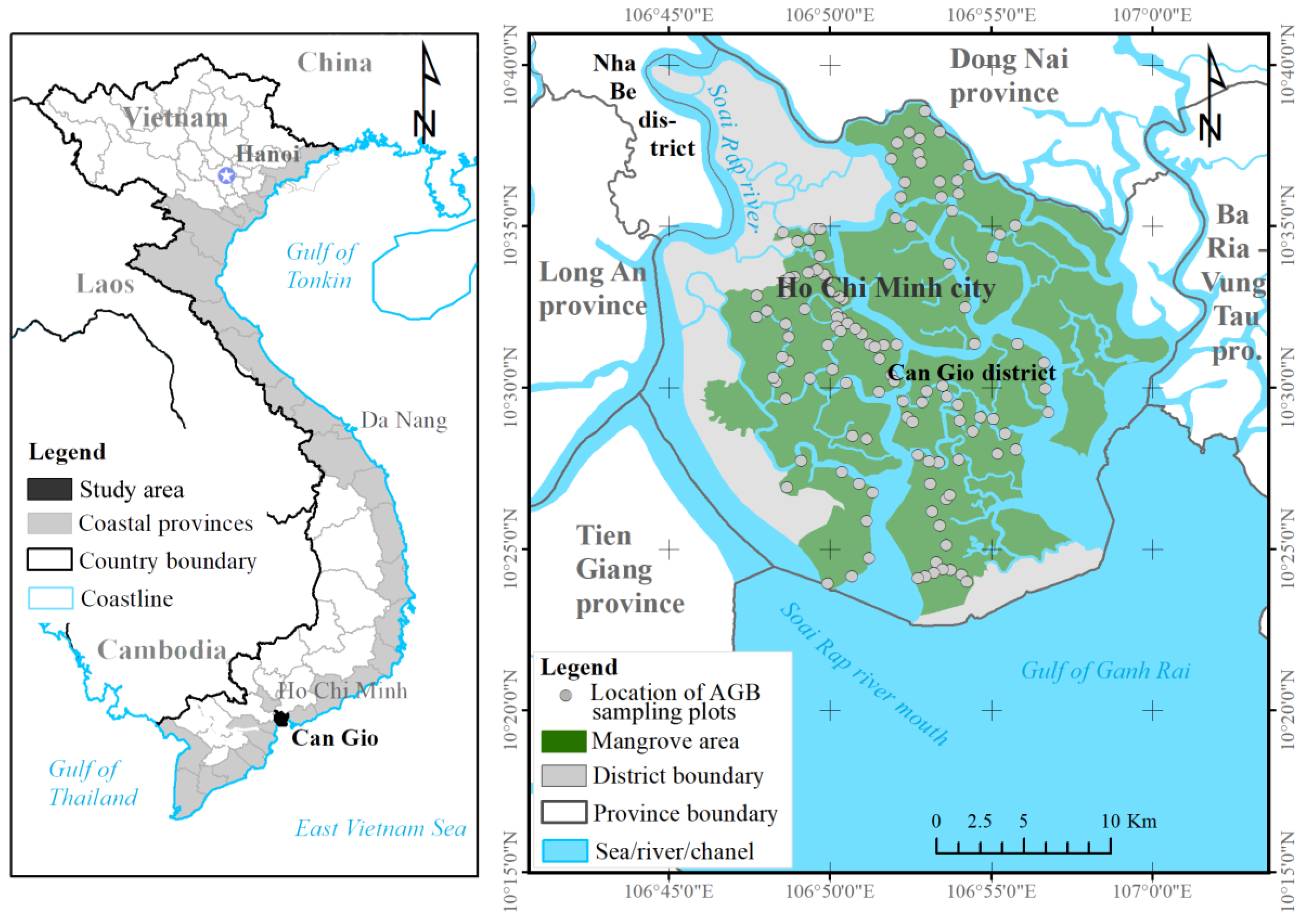
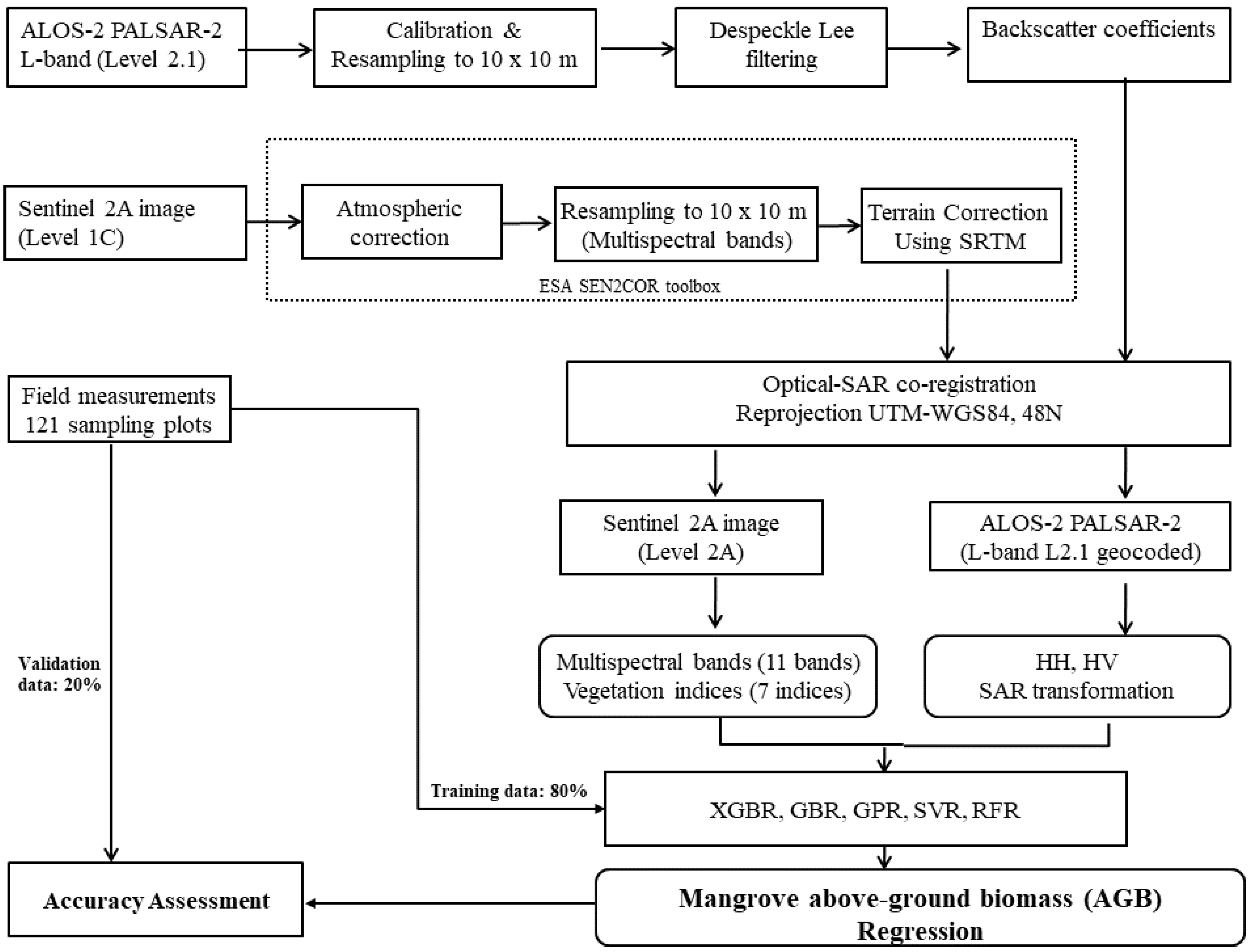
To overcome these challenges, we estimated the mangrove AGB in the Can Gio biosphere reserve (South Vietnam) using an ML model and the fused data of the Sentinel-2 (S2) MSI and ALOS-2 PALSAR-2 sensors. We selected Sentinel-2 MSI because the multispectral bands of S-2 reflect the forest stand structures such as stem volume, whereas the longer wavelengths of the dual polarimetric (HH, HV) mode of the ALOS-2 PALSAR-2 sensor can penetrate mangrove forest canopies. The fused S2 MSI and ALOS-2 PALSAR-2 data were processed by a nonlinear regression model in the XGBR algorithm, providing the first estimation of mangrove AGB in the Can Gio biosphere reserve (CGBRS). Additionally, the performance of the XGBR model was compared with those of other GBDT techniques and several well-known ML algorithms (SVR, GPR, and RFR) on mangrove AGB estimation in the same study area. Incorporating the S-2 MSI and ALOS-2 PALSAR-2 data into the proposed model was found to improve the mangrove AGB estimation in a Vietnamese biosphere reserve and is potentially applicable to mangrove conservation in other biosphere reserves.

2. Materials and Methods

2.1. Study Area

The present study was conducted in Can Gio, a coastal district located approximately 50 km south of Ho Chi Minh City (formerly Sai Gon) along the Southern coast of Vietnam. The geographical coordinates are 10°22′–10°40′ latitude and 106°46′–107°01′ longitude. The climate is tropical monsoon and has two typical seasons. The dry season begins in April and ends in November of the following year, whereas the rainy season occurs between May and October. The average temperature is approximately 26 °C, the annual rainfall is roughly 1300–1400 mm, and the relative humidity is approximately 80% [35]. This district is well-known for its mangrove reforestation and rehabilitation programs, not only in Vietnam but also throughout Southeast Asia [36]. The wetland ecosystem of Can Gio is diverse and includes the mangrove areas distributed in zone IV, which contains the largest mangrove forest among the four mangroves zones (See Figure 1) in Vietnam [37].

The Can Gio mangrove forests were declared as a biosphere reserve by the United Nations Educational, Scientific, and Cultural Organization (UNESCO) in 2000 [38]. The dominant species are Rhizophora apiculate, Sonneratia alba, Avicennia alba, Rhizophora mucronata, and others. Approximately 33 species belonging to 15 families have been identified in the CGBRS [36].

2.2. Field Survey Data Collection

With permission from the local authorities, the 2018 field survey of the CGBSR was conducted during the dry season, when the coastal tides impacting the mangrove forest were lowest. A total of 121 plots were sampled by the stratified random sampling approach. Each plot sampling was initially assisted by a local counterpart to guarantee the whole range of AGB values over the reserve. During the surveying, the experimenters measured the diameter at breast height (DBH), tree height (H), and tree density. All living mangrove forest stands with DBH > 5 cm in a strata plot size of 25 × 20 m (0.05 ha) were measured. The location (accuracy ± 2 m) of each sampling plot was measured by the Garmin eTrex global positioning system (GPS) (Figure 2).

The mangrove AGB of each species was estimated by a specific allometric equation (see

Table 1. Allometric equations for estimating the mangrove species in the study site.

Species	Allometric Equation	Reference
Rhizophora apiculata	AGB = 0.235 × DBH2.42 (R2 = 0.98)	[39]
Avicennia alba	AGB = 0.140 × DBH2.40 (R2 = 0.97)	[40]
Bruguiera gymnorrhiza	AGB = 0.186 × DBH2.31 (R2 = 0.99)	[41]
Bruguiera parviflora	AGB = 0.168 × DBH2.42 (R2 = 0.99)	[41]
Sonneratia caseolaris	AGB = 0.199 × φ × 0.90 * DBH2.22 (R2 = 0.99)	[40]
Lumnitzera racemosa	AGB = 0.740 × DBH2.32 (R2 = 0.99)	[42]
Ceriops zippeliana	AGB = 0.208 × DBH2.36 (R2 = 0.96)	[43]
Xylocarpus granatum	AGB = 0.082 × DBH2.59 (R2 = 0.99)	[41]

Note: AGB is the above-ground biomass (kg) of a mangrove tree, DBH is the diameter (cm) at breast height (1.3 m), φ is the wood density (tons dry matter per m³ fresh volume).

).

2.3. Remote Sensing Data Acquisition and Image Processing

2.3.1. Data Acquisition

The mangrove AGB in the CGBRS was estimated by fusing the ALOS-2 PALSAR-2 L-band dual polarimetric data level 2.1 obtained in high-sensitivity mode with Sentinel-2 (S-2) MSI images.

Table 2. Acquired earth observation data for this study.

Earth Observation Sensor	Scene ID	Acquisition Data	Processing Level	Spectral Band/Polarizations
ALOS-2 PALSAR-2	ALOS2206940200	23 March 2018	2.1	L band (HH, HV)
	ALOS2206940190
Sentinel-2 MSI	S2A_MSI_T48PXS	24 March 2018	1C	11 Multispectral bands
	S2A_MSI_T48PYS

presents the S-2 and the ALOS-2 PALSAR-2 data at the study site, acquired on 23 and 24 March during the 2018 dry seasons, respectively.

To pre-process the satellite remotely sensed data, we resampled both multispectral bands of Sentinel-2 and the dual polarization model of ALOS-2 PALSAR-2 data at a ground sampling distance (GSD) of 10 m. The satellite images were processed as described in Section 2.3.2. To validate the model’s performance and optimize the hyperparameters for AGB retrieval in the CGBRS, the model was combined with the measured field data. Figure 3 is a flowchart of the satellite-image processing and the generation of mangrove AGB estimation models using the ML techniques in the current study.

2.3.2. Satellite Image Processing

Two scenes of the ALOS-2 PALSAR-2 Level 2.1 data acquired on 23 March 2018 during the dry season were download from https://auig2.jaxa.jp/ips/home, the website of the Aerospace Exploration Agency (JAXA). The DN (Digital Number) of the ALOS-2 PALSAR-2 imagery was converted to normalized radar sigma-zero using Equation (1):

σ⁰ [dB] = 10. log10 (DN)² + CF

(1)

where σ⁰ is backscatter coefficients, and CF is the calibration factor. For HH and HV polarizations, CF = −83 dB [44]. Equation (1) converts the DN of each pixel to sigma naught (σ⁰) in decibel (dB).

Two scenes of the Sentinel-2 (S-2) Level-1C sensors acquired on 24 March 2018 during the dry season were retrieved from Copernicus Open Access Hub of the European Space Agency (ESA). The radiometric and geometric corrections of the S-2 data were made to the UTM/WGS84, Zone 48 North projection at top-of-atmosphere (TOA) reflectance [45]. The S-2 MSI Level-1C data were processed to Level-2A at the bottom-of-atmospheric (BOA) reflectance using the Sen2Cor algorithm of ESA (http://step.esa.int/main/third-party-plugins-2/sen2cor/). The S-2 and ALOS-2 PALSAR-2 images were processed by the SNAP toolbox, and the modeling process was performed in Python 3.7 environment using the Scikit-learn library [46].

2.3.3. Transformation of Multispectral and SAR Data

As a commonly employed method in previous mangrove AGB retrievals [13,47,48], image transformation was applied to the multispectral and SAR data of the present study. The image transformation of SAR data involves a combination of multi-polarizations such as HV/HH, HH/HV, and HH-HV, as suggested in [26]. Meanwhile, multispectral data are transformed using the vegetation indices, as each index is sensitive to mangrove structure and biomass.

Table 3. List of vegetation indices used in the current study.

Vegetation Index	Acronyms	Formula	References
Ratio Vegetation Index	RVI	$\frac{Band8}{Band4}$	[28]
Normalized Difference Vegetation Index	NDVI	$\frac{Band8-Band4}{Band8+Band4}$	[29]
Soil Adjusted Vegetation Index	SAVI	$\left(1+L\right)\left(\frac{Band8-Band4}{Band8+2.4Band4+L}\right)$ L = 0.5 in most conditions	[31]
Normalized Difference Index using bands 4 and 5 of Sentinel-2	NDI45	$\frac{Band5-Band4}{Band5+Band4}$	[32]
Difference Vegetation Index	DVI	Band 8–Band 4	[33]
Green Difference Vegetation Index	GNDVI	$\frac{Band8-Band3}{Band8+Band3}$	[34]
Inverted Red-Edge Chlorophyll Index	IRECl	$\frac{Band7-Band4}{Band5/Band6}$	[35]

shows the seven vegetation indices chosen for mangrove AGB retrieval at the CGBRS after referring to related studies [49,50,51]. The 23 predictor variables included five variables of ALOS-2 PALSAR-2 data (HV, HH, HV/HH, HH/HV, and HH-HV), 11 multispectral bands of S-2, and seven vegetation indices. Using the predictor variables, we computed the explanatory variables in the prediction model of mangrove AGB retrieval (Table 3). Figure 4 illustrates the image composites of different sensors and vegetation indices, along with the SAR transformation, in the study area.

2.4. Selection of Machine Learning Model

To identify the best model for AGB retrieval in CGBSR, we compared the performances of several ML techniques (XGBR, GBR, GPR, RFR, and SVR). The SVR model best predicted the mangrove AGB in a coastal area of North Vietnam [9], whereas the RFR model delivered the best monitoring results of mangrove biomass changes in South Vietnam [10]. Therefore, SVR and RFR were selected for the present study. The other ML algorithms were chosen because they are commonly used for solving regression problems in various fields [40,41,42].

2.4.1. Gradient Boosting Decision Trees Algorithms

a. Gradient Boosting Regression (GBR)

GBR is an ensemble-based decision tree method that boosts the performance of weak learners to those of stronger ones. Each regression tree of the GBR learns the residual of each tree conclusion. The main purpose is to reduce the previous residuals and thereby decrease the model residual along the gradient direction. The results of all regression trees are integrated to give the final result [52,53]. The GBR model can handle mixed data types and is robust to outliers [54]. As GBR has not been widely applied to mangrove biomass estimation, it was considered for testing in the present study.

The parameters to be determined are the learning rate, number of trees, minimum number of samples required at a leaf node, maximum depth, and the number of features for the best split. The hyperparameters of the GBR model were optimized by five-fold cross-validation (CV) techniques.

b. Extreme Gradient Boosting Regression (XGBR)

The Extreme Gradient Boosting (XGB) algorithm, proposed by Chen and Guestrin [55], is a novel GBR technique that develops strong learners by an additive training process. To resolve the drawbacks of weakly supervised learning, the additive learning is divided into two phases: A learning phase fitted to the entire input data, followed by adjustment to the residuals. The fitting process is repeated many times until the stopping criteria are achieved. This algorithm is based on “boosting decision trees”, which handle both classification and regression tasks in weakly supervised machine learning by the additive training strategies. The XGBR technique alleviates the undesired over-fitting problem.

The XGBR algorithm optimizes the loss function not by the first-order derivative (as in GBR) but by an efficient second-order expression. To avoid the over-fitting problem, the objective function treats the model complexity as a regularization term, and the regular term is added to the cost functions [55]. The XGBR model is quite generalizable and avoids both over-fitting and under-fitting. It also supports parallel computing to reduce computational time.

The parameters of XGBR are those of the GBR algorithm, and an additional parameter gamma (γ) representing the minimum loss of further partitioning a leaf node of the tree. The larger the γ, the more conservative is the algorithm. The XGBR model was also optimized by five-fold CV in the Python environment.

2.4.2. Support Vector Regression (SVR)

SVM is a supervised learning technique based on the statistical learning theory developed by Vapnik [56]. This method is widely used for classification and regression tasks in computer vision, pattern recognition, and environmental problems. SVR is an SVM method that solves specific regression problems. A nonlinear kernel function in SVR transforms the dataset into a higher dimensional feature space, where the data can be treated by simple linear regression. In this study, the selected kernel function was the radial basis function (RBF), the most widely adopted kernel for optimizing forest AGBs in prior studies [29,50].

The SVR model is generally configured by three hyperparameters: Epsilon (ε), the regulation parameter (C), and the kernel width (γ) of the RBF. In the present study, these parameters were optimized through five-fold CV.

2.4.3. Random Forests (RF)

RF [57] is the most common bagging model applied to both classification and regression problems. For training, RFR creates multiple uncorrelated trees from a randomly selected subset of 2/3 of the total samples (in-bag). The remaining 1/3 of the total samples (out-of-bag, OOB) are used for estimating the OOB error and validating the method. A tree is grown from in-bag samples with m features for optimizing the split at each node. In the absence of pruning, the tree reaches its largest possible extent. The RFR model produces (1) an OOB error and (2) the relative importance of each variable. From these outputs, it assesses the prediction accuracy and the contribution of each variable.

RFR is a high-performance non-parametric method that processes nonlinear data without overestimation during the training and testing phases. Accordingly, it has been widely employed in remote sensing [58,59]. The RFR requires the number of trees and the number of features m for the split. In this study, both RFR parameters were optimized by five-fold CV in the Python environment.

2.4.4. Gaussian Processes (GP)

Based on the non-parametric Bayesian theory, GPs are applicable to both classification and nonlinear regression problems. The GPR model learns the fit function from a small dataset using various kernels, finding the probability distribution that best describes the data. The input data are assumed to follow a multivariate Gaussian distribution, and the noise is independent of the data measurements [60]. The mean vector and covariance matrix are estimated from the training data by mean and covariance functions, respectively, creating a detailed posterior distribution from which the confidence interval and uncertainty of the prediction results can be interpreted. The mean value of a GP represents the best estimation from the model, and the variance (${\sigma }^2$) helps to measure the confidence level. GPs are well-known as good predictors of biophysical parameters [61].

2.5. Model Evaluation

2.5.1. Input Data for Model Running

To create the input data for training models, the 121 sampling plots were divided into training set (80%) and testing dataset (20%) using the well-known Scikit-learn [46] library in Python programming environment. Because the measured plot size (500 m²) greatly exceeded the image pixel size (10 m), all satellite data were smoothed through a median filter with a window size of 5 × 5 pixels in the SciPy library [62].

2.5.2. Hyperparameters Tuning in XGBR, GBR, RFR, SVR, and GPR

Hyperparameter tuning is often required when optimizing machine learning techniques. In this work, the parameters of each ML model were optimized by grid searching and five-fold CV. The results are listed in

Table 4. Optimized hyperparameters of the ML applied in this study.

Algorithm	Learning_Rate/Epsilon	Min_Samples_Leaf Min_Child_Weight	Gamma	Max_Depth/Max Features	n_Estimators or C Value
RFR	NA	2	NA	5, 15	50
SVR	0.01	NA	1000	NA	1000
GBR	0.2	5	NA	7, 3	100
XGBR	0.2	3	1	3	100

.

In the GPR, we combined the RBF with a length scale of 100 and WhiteKernel with a noise level of 1.0. The hyperparameters and kernels were maintained during the training and testing phases.

2.5.3. Feature Importance

The variables in RFR and gradient boosting machine algorithms, such as XGBR and GBR are often ranked by the variable-importance approach [55,63,64]. Relative variable importance is computed as follows. The first step searches for a candidate subset of variables (in this case, by the grid search approach). Initially, the grid search includes all variables derived from the S-2, VIs, and ALOS-2 PALSAR-2 datasets. The datasets are input to the XGBR model, which ranks the variables in descending order of their importance based on the root mean squared error (RMSE) and the coefficient of determination (R²). Next, a certain number of the least important variables are removed, and the surviving variables form a variable subset. In this paper, the search/selection iterations were terminated when the R² of the prediction model of the subset did not improve the performance in the test set. The final step validates the selected variable subset and determines the relative variable importance (in this case, by the five-fold CV approach).

The modeling and generated variable importance of the XGBR model were implemented in the Python environment.

2.5.4. Model Evaluation

The model performances of the various ML techniques were evaluated and compared by the RMSE (Equation (2)) and R² (Equation (3)), which are widely employed in estimates of forest AGB biomass. Both standards evaluate the errors in a regression model from the differences between the measured data (the mangrove forest measurements) and the estimated AGB data [50]. A well-performing model will achieve a high R² and a low [24,47].

$$\mathrm{RMSE}=\sqrt[]{{{\displaystyle \sum }}_1^n\frac{\left(y{e}_i-y{m}_i\right)2}{n}}$$

(2)

$$R^2=\frac{{\displaystyle {\sum }_{i=1}^n(y{e}_i-\overline{ye}})(y{m}_i-\overline{ym})}{\sqrt{{\displaystyle {\sum }_{i=1}^n(y{e}_i-\overline{ye}}{)}^2{(y{m}_i-\overline{ym})}^2}}$$

(3)

In the above expressions, $y{e}_i$ is the mangrove AGB predicted by the ML model, $y{m}_i$ is the measured mangrove AGB, n is the total number of sampling plots, and $\overline{ye}$ and $\overline{ym}$ are the mean values of the predicted and measured mangrove AGBs, respectively.

3. Results

3.1. Mangrove Tree Characteristics in CGBRS

Table 5. Characteristics of the mangrove trees in CGBRS.

Attribute	Min	Max	Mean	Standard Deviation (SD)
DBH (cm)	6.69	22.19	13.24	3.5
H (m)	6.47	17.35	11.87	2.5
Tree density (tree ha−1)	170	1680	694	26.45
AGB (Mg ha−1)	7.26	305.41	97.54	5.88

gives the characteristics of the mangrove trees in the 121 sampling plots. The AGBs ranged from 7.26 to 305.41 Mg ha⁻¹, with a mean of 97.54 Mg ha⁻¹. The mangrove heights varied from 6.47 to 17.35 m, and their DBHs ranged from 6.69 to 22.19 cm. The mangrove tree densities ranged from 170 to 1680 trees ha⁻¹ (Table 5).

3.2. Modeling Results, Assessment, and Comparison

Table 6. Performance comparison of ML techniques on mangrove AGB estimation.

No	Machine Learning Model	R2 Training (80%)	R2 Testing (20%)	RMSE (Mg ha−1)
1	Extreme Boosting regression (XGBR)	0.992	0.805	28.13
2	Gradient Boosting regression (GBR)	0.998	0.632	39.54
3	Random Forests regression (RFR)	0.721	0.468	48.44
4	Support Vector regression (SVR)	0.480	0.421	48.49
5	Gaussian Processes regression (GPR)	0.509	0.378	50.23

and Figure 5 compare the performances of the five regression methods with all input variables derived from S-2 MSI, VIs, and ALOS-2 PALSAR-2 images for mangrove AGB estimation in the study area. The XGBR model incorporating the S-2 (11 MS bands), ALOS- 2 PALSAR-2 (5 bands), and VIs (7 bands) data achieved the highest performance (Table 6), with an R² of 0.805 and an RMSE of 28.13 Mg ha⁻¹ in the testing dataset (23 predictor variables based on the fused S-2, the VIs and the ALOS-2 PALSAR-2 data), implying a good fit between the model estimates and field-based measurements. The next-highest performers were the GBR and RFR models. In contrast, the SVR and GPR models were unsuitable for retrieving the mangrove AGB at the study site (Table 6).

Table 7. Performance of the XGBR model using different numbers of variables. (Bold values highlight the best-performing model).

Scenario (SC)	Number of Variables	R2 Testing Set	RMSE (Mg ha−1)
SC1	11 variables from MS bands of S2 data	0.600	36.54
SC2	5 variables from ALOS-2 PALSAR-2 data	0.492	39.48
SC3	18 variables from MS bands and VIs from S2	0.739	34.86
SC4	23 variables (11 MS bands + 7 vegetation indices + 5 bands from ALOS-2 PALSAR-2)	0.805	28.13
SC5	16 variables (11 MS bands + 5 bands from ALOS-2 PALSAR-2)	0.656	43.25

lists the performances of the XGBR method in five scenarios (SCs) of mangrove AGB prediction, using different combinations of the S-2, ALOS-2 PALSAR-2, and VIs data.

As clarified in Table 7, the XGBR model yielded a promising result in SC3 using the combined S-2 and VIs, but the model achieved a poor result in SC2 using the ALOS-2 PALSAR-2 alone. The performance in SC1 using the S-2 dataset alone was moderate. We concluded that fusing all data in SC4 boosted the prediction performance of XGBR for estimating the mangrove AGB in the study area. The visual results of the testing phase (Figure 5) reconfirm the high performance of mangrove AGB estimation by XGBR with the 23 variables of the fused data. Particularly, the green scatter points cluster around the blue line and the RMSE is small.

3.3. Variable Importance

Among the multispectral bands of S-2 MSI, the Red (665 nm), Vegetation Red Edge (704 nm), and the narrow NIR (864 nm) spectra were most sensitive to the mangrove AGB of the present study, followed by the SWIR spectrum (MS band 11 at 1610 nm). Interestingly, among the seven VIs indices, the Inverted Red-Edge Chlorophyll Index (IRECl) and the Normalized Difference Index (NDI45) (bands 4 and 5 of S-2) were likely sensitive to the mangrove AGB in the study area. The band ratios derived from the incorporated HH and HH polarizations in the ALOS-2 PALSAR-2 data were also important for retrieving mangrove AGB in the biosphere reserve (see Figure 6). The backscatter coefficients of the crossed-polarimetric HV in ALOS-2 PALSAR-2 are likely more important than those of the HH for estimating the mangrove AGB in the study region (Figure 6).

3.4. Generation and Analysis of the AGB Map

The prediction performance of the XGBR model in mangrove AGB retrieval was improved by integrating the Sentinel-2 multispectral bands, vegetation indices, and ALOS-2 PALSAR-2 datasets. Thus, the XGBR model was selected for retrieving mangrove AGB in a biosphere reserve. The final results were computed to a raster in GeoTiff format for visualizing in QGIS. The AGB map was interpreted by seven classes (Figure 7), obtaining mangrove AGBs from 11 to 293 Mg ha⁻¹ (average = 106.93 Mg ha⁻¹). As can be seen from Figure 7, the biomass is highest in the core zone of the biosphere reserve and lower in the transition and buffer zones. These results are consistent with prior mangrove AGB estimates [17] and [65], in which the high biomass was mainly distributed in the core zone of the biosphere reserve, and the lower biomass was observed in the remaining zones.

4. Discussion

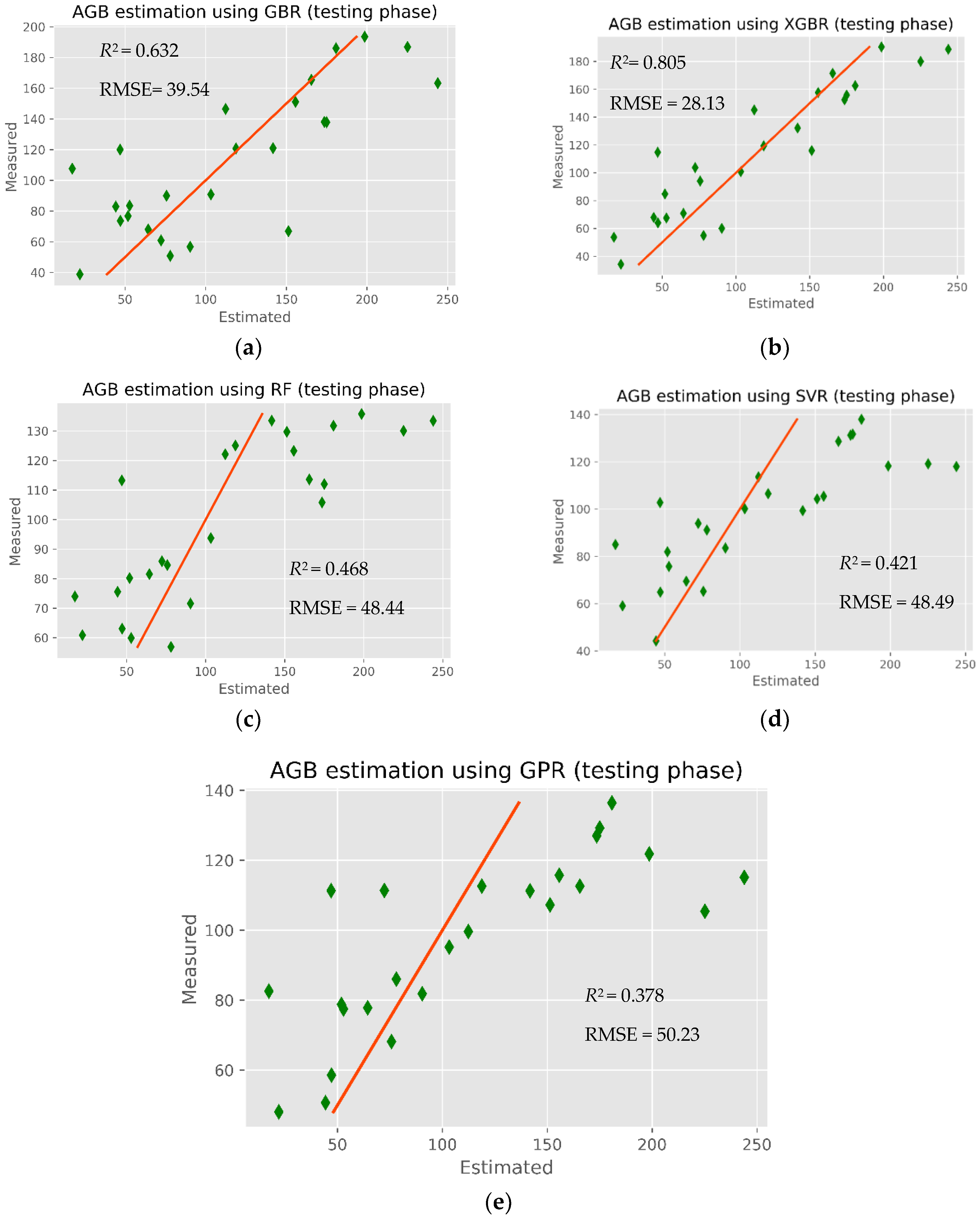
The modeling results of mangrove AGB retrieval in the CGBSR obtained by the five ML models (XGBR, GBR, GPR, SVR, and RFR) are given in Table 6. Clearly, the XGBR model yielded the highest performance, with an R² and RMSE of 0.805 and 28.13 Mg ha⁻¹, respectively. The worst performing model was GPR, with an R² and RMSE of 0.378 and 50.23 Mg ha⁻¹, respectively. Both the XGBR model (R² = 0.805) and GBR model (R² = 0.632) were good predictors of mangrove AGB, indicating that the GBDT regression models were applicable to the study area, where the mangrove biomass is higher than in other mangrove regions of Vietnam. As shown in Table 7, the combined S-2 and ALOS-2 PALSAR data significantly improved the performance of estimating the mangrove AGB in the study area. These results are consistent with a recent previous study [50]. Overall, the XGBR model outperformed the existing algorithms in retrieving the mangrove AGB in a Vietnamese biosphere reserve.

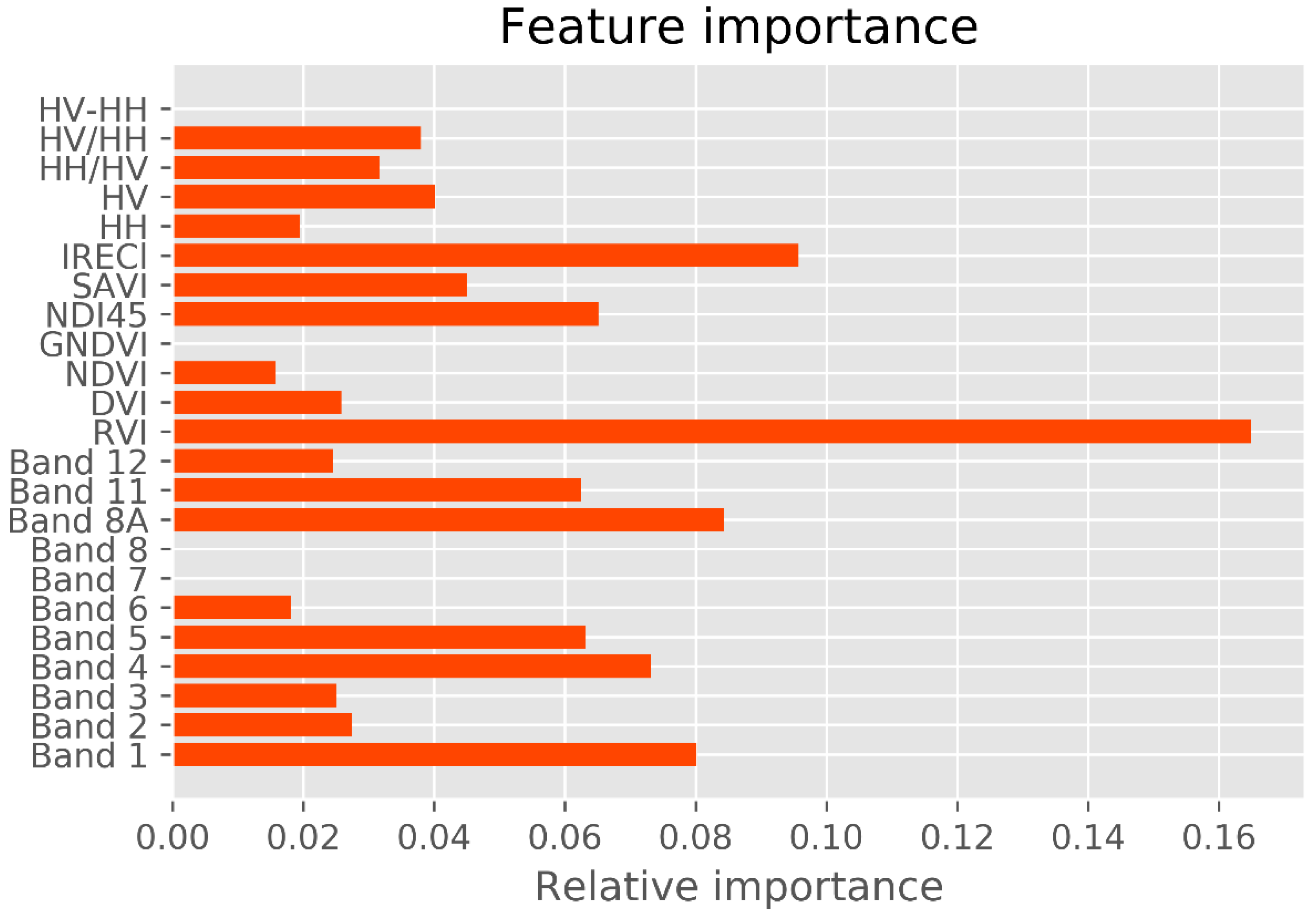
Previous studies reported that long-wavelength PolSAR data, such as the L and the P bands, are well correlated with mangrove forest structures. Among these data, crossed-polarized HV appears to be most correlated with biophysical attributes [13,66,67]. The variable-importance analysis revealed that crossed-polarization HV is more sensitive to mangrove AGB in the study area than HH polarization (Figure 6), consistent with previous results [26,29]. However, mangrove forests in a biosphere reserve exhibit unique stand structures and species compositions that may saturate multispectral and SAR sensors. Data saturation of multispectral sensors such as Landsat TM, ETM+ or OLI, and the S-2 sensor degrades the prediction accuracy of mangrove AGBs in dense forest canopies. The saturation range of multispectral data reaches 100–150 Mg ha⁻¹ in complex tropical forests, much higher than in mixed and pine forest ecosystems (with a saturation range of >150 to <160 Mg ha⁻¹) [68,69]. In several recent investigations, the saturation levels of the mangrove AGBs retrieved from SAR data ranged from above 100 Mg ha⁻¹ [20] to below 150 Mg ha⁻¹ [21,26]. This large range probably manifests from the root systems of different mangrove species in intertidal tropical and sub-tropical regions [13]. The sigma backscatter coefficients of the dual polarimetric data of ALOS-2 PALSAR-2 increased when the mangrove AGB fell below 100 Mg ha⁻¹ and then saturated at a higher AGB because the high mangrove cover density extinguished the radar signals [70,71].

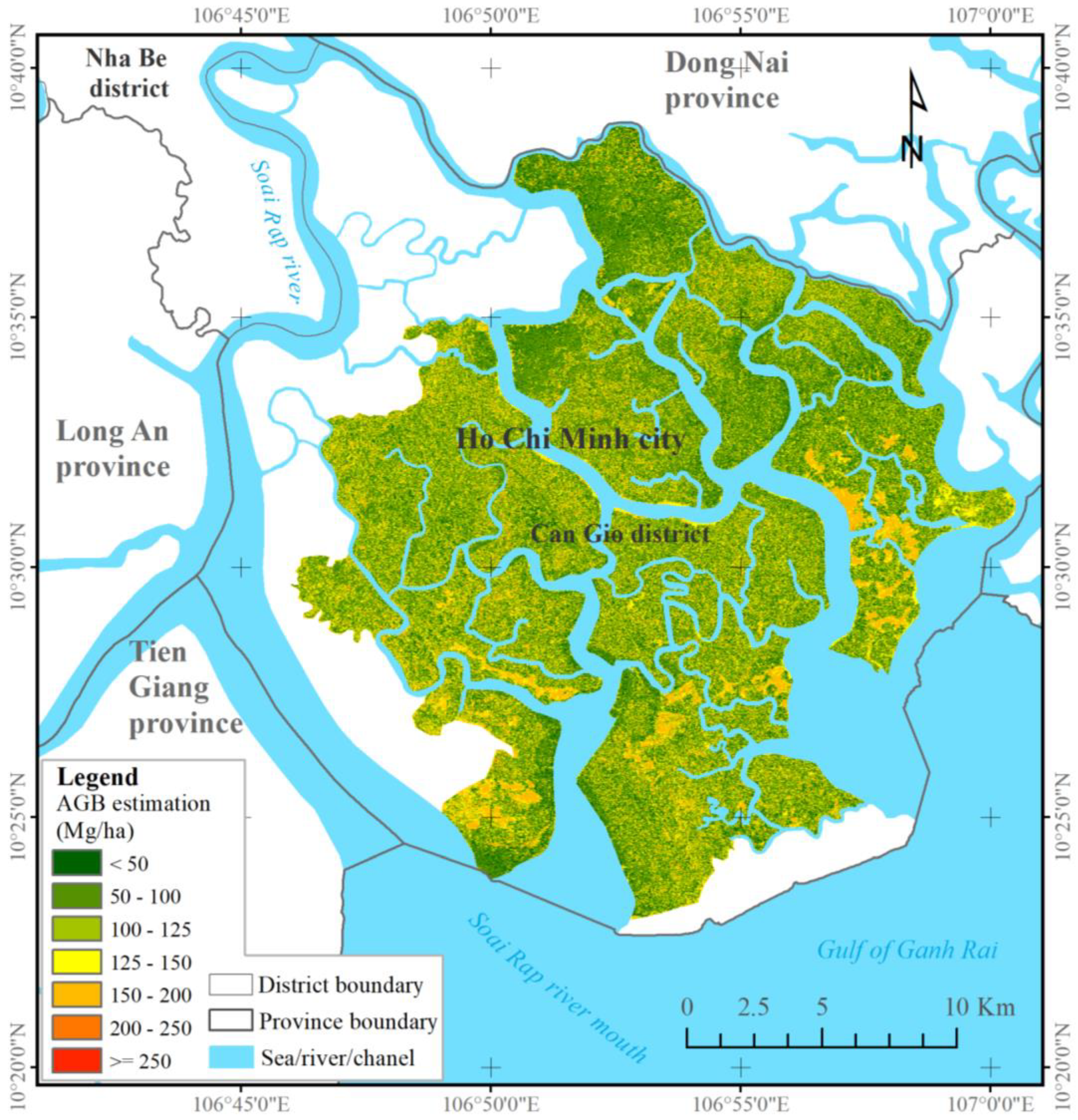
Biosphere reserves often consist of various mangrove species. The species types (i.e., R. appiculata, B. gymnorrhiza, and S. caseolaris) are densely grown and characterized by high DBH and tall height. Some species, such as A. germinans and C. decandra, form small but high-density mangrove patches in which high and low biomasses are easily underestimated and overestimated, respectively, by machine learning algorithms. In the current study, the XGBR model possibly over-estimated the low mangrove AGBs (below 50 Mg ha⁻¹) and under-estimated the high values (over 250 Mg ha⁻¹). Despite these limitations, the combined ALOS-2 PALSAR-2 and S-2 data sensitively detected mangrove AGBs exceeding 200 Mg ha⁻¹ in the CGBRS (See Figure 5). Our findings agree with the conclusions of prior research on biosphere reserves [17,65]. Given the species complexity in mangrove biosphere reserves, we recommend the inclusion of species classification or richness indices for improved mangrove AGB estimation in future work [19,21].

In the variable-importance results, the mangrove AGB in the study area was largely retrieved from the Red band and the Vegetation Red Edge band. A similar result was reported elsewhere [18,72]. The vegetation red edge, narrow NIR, and SWIR reflectance are likely to be more strongly correlated with forest biomass and carbon stock volume than visible reflectance [17]. Accordingly, the new vegetation index ND145, which is computed from the Sentinel-2 data bands, is a probable sensitive indicator of mangrove AGB. Band 8A in the narrow NIR and band 11 in the SWIR (1613 nm) also played a crucial role in the AGB retrieval. Interestingly, the IRECl derived from S-2 was strongly correlated with mangrove AGB in the biosphere reserve. More in-depth studies would elucidate the effectiveness of image transformations involving new vegetation indices derived from the Narrow NIR bands, SWIR of S-2 data, and other image transformations computed from the fully polarized data (HH, HV, VH, and VV) of the Gaofeng-3 and the ALOS-2 PALSAR-2 sensors in biosphere reserves.

To accurately estimate mangrove AGBs, researchers attempted multi-linear regression, which performed poorly with R² ranging from 0.43–0.65 [13,21,73], and various ML algorithms such as GPR, MLPNN, SVR, and RFR [17,18,29]. ML approaches have proven more successful in mangrove AGB than multi-linear regression and other parametric methods [18,47], but the R² has rarely exceeded 0.70. Therefore, novel approaches for mangrove AGB estimation are urgently needed. In this research, the performance of the XGBR model was boosted by incorporating data from the ALOS-2 PALSAR-2, S-2 sensors. The result (R² = 0.805 for the AGB of a mangrove biosphere reserve in the tropics) demonstrates the promise of this approach. Despite the good fit between the XGBR-predicted and measured-mean mangrove AGBs, the range of the predicted mangrove AGBs did not reach the extrema of the actual distribution range, which was maximized at 305.41 Mg ha⁻¹ and minimized at 26 Mg ha⁻¹ (Table 5). The predicted results may have been degraded by the saturation levels of the S2 MSI sensor and the dual polarimetric L-band ALOS-2 PALSAR-2 when retrieving mangrove AGB in intertidal areas. Although the AGB was well predicted by the XGBR model, the R² values in the training and testing phases were significantly different (Table 6). This difference is likely attributable to the mixed mangrove species planted in the CGBRS and the number of plots. To archive a more accurate forest AGB map, we should exploit the advantages of various novel GBDT algorithms with multi-sensor data integration [74]. In more intensive works, novel boosting decision tree techniques should exploit the full capability of multi-source EO data in different mangrove communities occupying tropical intertidal areas at different geographical locations, particularly those of biosphere reserves. Such developments are needed for rapid mangrove AGB monitoring in the future.

5. Conclusions

We report the first attempt to incorporate Sentinel-2 and ALOS-2 PALSAR-2 data into the extreme gradient boosting regression (XGBR) model and thereby estimate the mangrove AGB in Vietnam’s Can Gio biosphere reserve. The XGBR model outperformed four other machine learning models in mangrove AGB retrieval in the study area. When provided with the Sentinel-2 and ALOS-2 PALSAR-2 data, XGBR estimated the mangrove AGB with satisfactory accuracy (R² = 0.805, RMSE = 28.13 Mg ha⁻¹). Interestingly, we found that new vegetation indices derived from the Sentinel-2 data, such as the Normalized Difference Index (NDI45) and the Inverted Red-Edge Chlorophyll Index (IRECl), sensitively detected mangrove AGB in the biosphere reserve. In future investigations, the proposed approach should be tested in other tropical forest ecosystems.

References

1. Alongi, D.M. Carbon sequestration in mangrove forests. Carbon Manag. 2012, 3, 313–322. [Google Scholar] [CrossRef]
2. Brander, L.M.; Wagtendonk, A.J.; Hussain, S.S.; McVittie, A.; Verburg, P.H.; de Groot, R.S.; van der Ploeg, S. Ecosystem service values for mangroves in Southeast Asia: A meta-analysis and value transfer application. Ecosyst. Serv. 2012, 1, 62–69. [Google Scholar] [CrossRef] [Green Version]
3. Richards, D.R.; Friess, D.A. Rates and drivers of mangrove deforestation in Southeast Asia, 2000–2012. Proc. Natl. Acad. Sci. USA 2016, 113, 344–349. [Google Scholar] [CrossRef] [PubMed] [Green Version]
4. Friess, D.A.; Rogers, K.; Lovelock, C.E.; Krauss, K.W.; Hamilton, S.E.; Lee, S.Y.; Lucas, R.; Primavera, J.; Rajkaran, A.; Shi, S. The State of the World’s Mangrove Forests: Past, Present, and Future. Annu. Rev. Environ. Resour. 2019, 44, 89–115. [Google Scholar] [CrossRef] [Green Version]
5. Pham, T.D.; Yoshino, K. Impacts of mangrove management systems on mangrove changes in the Northern Coast of Vietnam. Tropics 2016, 24, 141–151. [Google Scholar] [CrossRef] [Green Version]
6. Friess, D.A.; Webb, E.L. Variability in mangrove change estimates and implications for the assessment of ecosystem service provision. Glob. Ecol. Biogeogr. 2014, 23, 715–725. [Google Scholar] [CrossRef]
7. Lv, Z.Y.; Liu, T.F.; Zhang, P.; Benediktsson, J.A.; Lei, T.; Zhang, X. Novel Adaptive Histogram Trend Similarity Approach for Land Cover Change Detection by Using Bitemporal Very-High-Resolution Remote Sensing Images. IEEE Trans. Geosci. Remote Sens. 2019, 57, 9554–9574. [Google Scholar] [CrossRef]
8. Zhao, T.; Bergen, K.M.; Brown, D.G.; Shugart, H.H. Scale dependence in quantification of land-cover and biomass change over Siberian boreal forest landscapes. Landsc. Ecol. 2009, 24, 1299. [Google Scholar] [CrossRef]
9. Lv, Z.; Liu, T.; Zhang, P.; Atli Benediktsson, J.; Chen, Y. Land Cover Change Detection Based on Adaptive Contextual Information Using Bi-Temporal Remote Sensing Images. Remote Sens. 2018, 10, 901. [Google Scholar] [CrossRef] [Green Version]
10. Clough, B.F.; Dixon, P.; Dalhaus, O. Allometric Relationships for Estimating Biomass in Multi-stemmed Mangrove Trees. Aust. J. Bot. 1997, 45, 1023–1031. [Google Scholar] [CrossRef]
11. Komiyama, A.; Ong, J.E.; Poungparn, S. Allometry, biomass, and productivity of mangrove forests: A review. Aquat. Bot. 2008, 89, 128–137. [Google Scholar] [CrossRef]
12. Hirata, Y.; Tabuchi, R.; Patanaponpaiboon, P.; Poungparn, S.; Yoneda, R.; Fujioka, Y. Estimation of aboveground biomass in mangrove forests using high-resolution satellite data. J. For. Res. 2014, 19, 34–41. [Google Scholar] [CrossRef]
13. Hamdan, O.; Khali Aziz, H.; Mohd Hasmadi, I. L-band ALOS PALSAR for biomass estimation of Matang Mangroves, Malaysia. Remote Sens. Environ. 2014, 155, 69–78. [Google Scholar] [CrossRef]
14. Darmawan, S.; Takeuchi, W.; Vetrita, Y.; Wikantika, K.; Sari, D.K. Impact of Topography and Tidal Height on ALOS PALSAR Polarimetric Measurements to Estimate Aboveground Biomass of Mangrove Forest in Indonesia. J. Sens. 2015, 2015, 13. [Google Scholar] [CrossRef] [Green Version]
15. Kauffman, J.B.; Donato, D.C. Protocols for the Measurement, Monitoring and Reporting of Structure, Biomass, and Carbon Stocks in Mangrove Forests; CIFOR: Bogor, Indonesia, 2012. [Google Scholar]
16. Ahmed, N.; Glaser, M. Coastal aquaculture, mangrove deforestation and blue carbon emissions: Is REDD+ a solution? Mar. Policy 2016, 66, 58–66. [Google Scholar] [CrossRef]
17. Pham, L.T.H.; Brabyn, L. Monitoring mangrove biomass change in Vietnam using SPOT images and an object-based approach combined with machine learning algorithms. ISPRS J. Photogramm. Remote Sens. 2017, 128, 86–97. [Google Scholar] [CrossRef]
18. Jachowski, N.R.A.; Quak, M.S.Y.; Friess, D.A.; Duangnamon, D.; Webb, E.L.; Ziegler, A.D. Mangrove biomass estimation in Southwest Thailand using machine learning. Appl. Geogr. 2013, 45, 311–321. [Google Scholar] [CrossRef]
19. Zhu, Y.; Liu, K.; Liu, L.; Wang, S.; Liu, H. Retrieval of Mangrove Aboveground Biomass at the Individual Species Level with WorldView-2 Images. Remote Sens. 2015, 7, 12192–12214. [Google Scholar] [CrossRef] [Green Version]
20. Lucas, R.M.; Mitchell, A.L.; Rosenqvist, A.; Proisy, C.; Melius, A.; Ticehurst, C. The potential of L-band SAR for quantifying mangrove characteristics and change: Case studies from the tropics. Aquat. Conserv. Mar. Freshw. Ecosyst. 2007, 17, 245–264. [Google Scholar] [CrossRef]
21. Pham, T.D.; Yoshino, K. Aboveground biomass estimation of mangrove species using ALOS-2 PALSAR imagery in Hai Phong City, Vietnam. APPRES 2017, 11, 026010. [Google Scholar] [CrossRef]
22. Maeda, Y.; Fukushima, A.; Imai, Y.; Tanahashi, Y.; Nakama, E.; Ohta, S.; Kawazoe, K.; Akune, N. Estimating carbon stock changes of mangrove forests using satellite imagery and airborne lidar data in the south Sumatra state, Indonesia. ISPRS Int. Arch. Photogramm. Remote Sens. Spat. Inf. Sci. 2016, 705–709. [Google Scholar] [CrossRef]
23. Fatoyinbo, T.; Feliciano, E.A.; Lagomasino, D.; Lee, S.K.; Trettin, C. Estimating mangrove aboveground biomass from airborne LiDAR data: A case study from the Zambezi River delta. Environ. Res. Lett. 2018, 13, 025012. [Google Scholar] [CrossRef] [Green Version]
24. Wang, D.; Wan, B.; Liu, J.; Su, Y.; Guo, Q.; Qiu, P.; Wu, X. Estimating aboveground biomass of the mangrove forests on northeast Hainan Island in China using an upscaling method from field plots, UAV-LiDAR data and Sentinel-2 imagery. Int. J. Appl. Earth Obs. Geoinf. 2020, 85, 101986. [Google Scholar] [CrossRef]
25. Wang, D.; Wan, B.; Qiu, P.; Zuo, Z.; Wang, R.; Wu, X. Mapping Height and Aboveground Biomass of Mangrove Forests on Hainan Island Using UAV-LiDAR Sampling. Remote Sens. 2019, 11, 2156. [Google Scholar] [CrossRef] [Green Version]
26. Pham, T.D.; Yoshino, K.; Bui, D.T. Biomass estimation of Sonneratia caseolaris (L.) Engler at a coastal area of Hai Phong city (Vietnam) using ALOS-2 PALSAR imagery and GIS-based multi-layer perceptron neural networks. Gisci. Remote Sens. 2017, 54, 329–353. [Google Scholar] [CrossRef]
27. Wu, C.; Shen, H.; Shen, A.; Deng, J.; Gan, M.; Zhu, J.; Xu, H.; Wang, K. Comparison of machine-learning methods for above-ground biomass estimation based on Landsat imagery. APPRES 2016, 10, 035010. [Google Scholar] [CrossRef]
28. López-Serrano, P.M.; López-Sánchez, C.A.; Álvarez-González, J.G.; García-Gutiérrez, J. A Comparison of Machine Learning Techniques Applied to Landsat-5 TM Spectral Data for Biomass Estimation. Can. J. Remote Sens. 2016, 42, 690–705. [Google Scholar] [CrossRef]
29. Pham, T.D.; Yoshino, K.; Le, N.; Bui, D. Estimating Aboveground Biomass of a Mangrove Plantation on the Northern coast of Vietnam using machine learning techniques with an integration of ALOS-2 PALSAR-2 and Sentinel-2A data. Int. J. Remote Sens. 2018, 39, 7761–7788. [Google Scholar] [CrossRef]
30. Huang, G.; Wu, L.; Ma, X.; Zhang, W.; Fan, J.; Yu, X.; Zeng, W.; Zhou, H. Evaluation of CatBoost method for prediction of reference evapotranspiration in humid regions. J. Hydrol. 2019, 574, 1029–1041. [Google Scholar] [CrossRef]
31. Gumus, M.; Kiran, M.S. Crude oil price forecasting using XGBoost. In Proceedings of the 2017 International Conference on Computer Science and Engineering (UBMK), Antalya, Turkey, 5–7 October 2017; pp. 1100–1103. [Google Scholar]
32. Sun, Y.; Gao, C.; Li, J.; Wang, R.; Liu, J. Evaluating urban heat island intensity and its associated determinants of towns and cities continuum in the Yangtze River Delta Urban Agglomerations. Sustain. Cities Soc. 2019, 50, 101659. [Google Scholar] [CrossRef]
33. Ghatkar, J.G.; Singh, R.K.; Shanmugam, P. Classification of algal bloom species from remote sensing data using an extreme gradient boosted decision tree model. Int. J. Remote Sens. 2019, 40, 9412–9438. [Google Scholar] [CrossRef]
34. Li, P.; Zhang, J.-S. A New Hybrid Method for China’s Energy Supply Security Forecasting Based on ARIMA and XGBoost. Energies 2018, 11, 1687. [Google Scholar] [CrossRef] [Green Version]
35. Veettil, B.K.; Ward, R.D.; Quang, N.X.; Trang, N.T.T.; Giang, T.H. Mangroves of Vietnam: Historical development, current state of research and future threats. Estuar. Coast. Shelf Sci. 2019, 218, 212–236. [Google Scholar] [CrossRef]
36. Tuan, L.D.; Oanh, T.T.K.; Thanh, C.V.; Quy, N.D. Can Gio Mangrove Biosphere Reserve; Agricultural Publishing House: Ho Chi Minh City, Vietnam, 2002; p. 311. [Google Scholar]
37. Hong, P.N.; San, H.T. Mangroves of Vietnam; IUCN: Bangkok, Thailand, 1993; p. 173. [Google Scholar]
38. Vogt, J.; Kautz, M.; Fontalvo Herazo, M.L.; Triet, T.; Walther, D.; Saint-Paul, U.; Diele, K.; Berger, U. Do canopy disturbances drive forest plantations into more natural conditions?—A case study from Can Gio Biosphere Reserve, Viet Nam. Glob. Planet. Chang. 2013, 110, 249–258. [Google Scholar] [CrossRef]
39. Ong, J.E.; Gong, W.K.; Wong, C.H. Allometry and partitioning of the mangrove, Rhizophora apiculata. For. Ecol. Manag. 2004, 188, 395–408. [Google Scholar] [CrossRef]
40. Komiyama, A.; Poungparn, S.; Kato, S. Common allometric equations for estimating the tree weight of mangroves. J. Trop. Ecol. 2005, 21, 471–477. [Google Scholar] [CrossRef]
41. Clough, B.F.; Scott, K. Allometric relationships for estimating above-ground biomass in six mangrove species. For. Ecol. Manag. 1989, 27, 117–127. [Google Scholar] [CrossRef]
42. Kangkuso, A.; Jamili, J.; Septiana, A.; Raya, R.; Sahidin, I.; Rianse, U.; Rahim, S.; Alfirman, A.; Sharma, S.; Nadaoka, K. Allometric models and aboveground biomass of Lumnitzera racemosa Willd. forest in Rawa Aopa Watumohai National Park, Southeast Sulawesi, Indonesia. For. Sci. Technol. 2016, 12, 43–50. [Google Scholar] [CrossRef] [Green Version]
43. Binh, C.H.; Nam, V.N. Carbon sequestration of Ceriops zippeliana in Can Gio mangroves. In Studies in Can Gio Mangrove Biosphere Reserve, Ho Chi Minh City, Viet Nam; ISME: Okinawa, Japan, 2014; p. 51. [Google Scholar]
44. Shimada, M.; Isoguchi, O.; Tadono, T.; Isono, K. PALSAR Radiometric and Geometric Calibration. IEEE Trans. Geosci. Remote Sens. 2009, 47, 3915–3932. [Google Scholar] [CrossRef]
45. Drusch, M.; Del Bello, U.; Carlier, S.; Colin, O.; Fernandez, V.; Gascon, F.; Hoersch, B.; Isola, C.; Laberinti, P.; Martimort, P.; et al. Sentinel-2: ESA’s Optical High-Resolution Mission for GMES Operational Services. Remote Sens. Environ. 2012, 120, 25–36. [Google Scholar] [CrossRef]
46. Pedregosa, F.; Varoquaux, G.; Gramfort, A.; Michel, V.; Thirion, B.; Grisel, O.; Blondel, M.; Prettenhofer, P.; Weiss, R.; Dubourg, V. Scikit-learn: Machine learning in Python. J. Mach. Learn. Res. 2011, 12, 2825–2830. [Google Scholar]
47. Navarro, J.A.; Algeet, N.; Fernández-Landa, A.; Esteban, J.; Rodríguez-Noriega, P.; Guillén-Climent, M.L. Integration of UAV, Sentinel-1, and Sentinel-2 Data for Mangrove Plantation Aboveground Biomass Monitoring in Senegal. Remote Sens. 2019, 11. [Google Scholar] [CrossRef] [Green Version]
48. Castillo, J.A.A.; Apan, A.A.; Maraseni, T.N.; Salmo, S.G. Estimation and mapping of above-ground biomass of mangrove forests and their replacement land uses in the Philippines using Sentinel imagery. ISPRS J. Photogramm. Remote Sens. 2017, 134, 70–85. [Google Scholar] [CrossRef]
49. Patil, V.; Singh, A.; Naik, N.; Unnikrishnan, S. Estimation of Mangrove Carbon Stocks by Applying Remote Sensing and GIS Techniques. Wetlands 2015, 35, 695–707. [Google Scholar] [CrossRef]
50. Vafaei, S.; Soosani, J.; Adeli, K.; Fadaei, H.; Naghavi, H.; Pham, T.D.; Tien Bui, D. Improving Accuracy Estimation of Forest Aboveground Biomass Based on Incorporation of ALOS-2 PALSAR-2 and Sentinel-2A Imagery and Machine Learning: A Case Study of the Hyrcanian Forest Area (Iran). Remote Sens. 2018, 10, 172. [Google Scholar] [CrossRef] [Green Version]
51. Ghosh, S.M.; Behera, M.D. Aboveground biomass estimation using multi-sensor data synergy and machine learning algorithms in a dense tropical forest. Appl. Geogr. 2018, 96, 29–40. [Google Scholar] [CrossRef]
52. Friedman, J.H. Greedy function approximation: A gradient boosting machine. Ann. Stat. 2001, 29, 1189–1232. [Google Scholar] [CrossRef]
53. Friedman, J.H. Stochastic gradient boosting. Comput. Stat. Data Anal. 2002, 38, 367–378. [Google Scholar] [CrossRef]
54. Wei, Z.; Meng, Y.; Zhang, W.; Peng, J.; Meng, L. Downscaling SMAP soil moisture estimation with gradient boosting decision tree regression over the Tibetan Plateau. Remote Sens. Environ. 2019, 225, 30–44. [Google Scholar] [CrossRef]
55. Chen, T.; Guestrin, C. Xgboost: A scalable tree boosting system. In Proceedings of the 22nd Acm Sigkdd International Conference on Knowledge Discovery and Data Mining, San Francisco, CA, USA, 13–17 August 2016; ACM: New York, NY, USA; pp. 785–794. [Google Scholar]
56. Vapnik, V. The Nature of Statistical Learning Theory; Springer Science & Business Media: Berlin/Heidelberg, Germany, 2013. [Google Scholar]
57. Breiman, L. Random Forests. Mach. Learn. 2001, 45, 5–32. [Google Scholar] [CrossRef] [Green Version]
58. Belgiu, M.; Drăguţ, L. Random forest in remote sensing: A review of applications and future directions. ISPRS J. Photogramm. Remote Sens. 2016, 114, 24–31. [Google Scholar] [CrossRef]
59. Pham, T.D.; Xia, J.; Baier, G.; Le, N.N.; Yokoya, N. Mangrove Species Mapping Using Sentinel-1 and Sentinel-2 Data in North Vietnam. In Proceedings of the IGARSS 2019—2019 IEEE International Geoscience and Remote Sensing Symposium, Yokohama, Japan, 28 July–2 August 2019; pp. 6102–6105. [Google Scholar]
60. Perez-Cruz, F.; Vaerenbergh, S.V.; Murillo-Fuentes, J.J.; Lazaro-Gredilla, M.; Santamaria, I. Gaussian Processes for Nonlinear Signal Processing: An Overview of Recent Advances. IEEE Signal. Process. Mag. 2013, 30, 40–50. [Google Scholar] [CrossRef] [Green Version]
61. Rasmussen, C.E.; Williams, C.K. Gaussian Processes for Machine Learning; MIT Press: Cambridge, MA, USA, 2006; Volume 1. [Google Scholar]
62. Jones, E.; Oliphant, T.; Peterson, P. SciPy: Open Source Scientific Tools for Python. 2001. Available online: https://www.scienceopen.com/document?vid=ab12905a-8a5b-43d8-a2bb-defc771410b9 (accessed on 4 August 2019).
63. Grömping, U. Variable Importance Assessment in Regression: Linear Regression versus Random Forest. Am. Stat. 2009, 63, 308–319. [Google Scholar] [CrossRef]
64. Li, Y.; Li, C.; Li, M.; Liu, Z. Influence of Variable Selection and Forest Type on Forest Aboveground Biomass Estimation Using Machine Learning Algorithms. Forests 2019, 10, 1073. [Google Scholar] [CrossRef] [Green Version]
65. Nguyen Viet, L.; To Trong, T.; Luong Anh, K.; Nguyen Thanh, H. Biomass estimation and mapping of can GIO mangrove biosphere reserve in south of viet nam using ALOS-2 PALSAR-2 data. Appl. Ecol. Environ. Res. 2019, 17, 15–31. [Google Scholar]
66. Lucas, R.; Armston, J.; Fairfax, R.; Fensham, R.; Accad, A.; Carreiras, J.; Kelley, J.; Bunting, P.; Clewley, D.; Bray, S.; et al. An Evaluation of the ALOS PALSAR L-Band Backscatter-Above Ground Biomass Relationship Queensland, Australia: Impacts of Surface Moisture Condition and Vegetation Structure. IEEE J. Sel. Top. Appl. Earth Obs. Remote Sens. 2010, 3, 576–593. [Google Scholar] [CrossRef]
67. Schlund, M.; Davidson, M. Aboveground Forest Biomass Estimation Combining L- and P-Band SAR Acquisitions. Remote Sens. 2018, 10, 1151. [Google Scholar] [CrossRef] [Green Version]
68. Foody, G.M.; Boyd, D.S.; Cutler, M.E.J. Predictive relations of tropical forest biomass from Landsat TM data and their transferability between regions. Remote Sens. Environ. 2003, 85, 463–474. [Google Scholar] [CrossRef]
69. Cutler, M.E.J.; Boyd, D.S.; Foody, G.M.; Vetrivel, A. Estimating tropical forest biomass with a combination of SAR image texture and Landsat TM data: An assessment of predictions between regions. ISPRS J. Photogramm. Remote Sens. 2012, 70, 66–77. [Google Scholar] [CrossRef] [Green Version]
70. Proisy, C.; Couteron, P.; Fromard, F. Predicting and mapping mangrove biomass from canopy grain analysis using Fourier-based textural ordination of IKONOS images. Remote Sens. Environ. 2007, 109, 379–392. [Google Scholar] [CrossRef]
71. Joshi, N.; Mitchard, E.T.A.; Brolly, M.; Schumacher, J.; Fernández-Landa, A.; Johannsen, V.K.; Marchamalo, M.; Fensholt, R. Understanding ‘saturation’ of radar signals over forests. Sci. Rep. 2017, 7, 3505. [Google Scholar] [CrossRef] [PubMed] [Green Version]
72. Chrysafis, I.; Mallinis, G.; Siachalou, S.; Patias, P. Assessing the relationships between growing stock volume and Sentinel-2 imagery in a Mediterranean forest ecosystem. Remote Sens. Lett. 2017, 8, 508–517. [Google Scholar] [CrossRef]
73. Wicaksono, P.; Danoedoro, P.; Hartono; Nehren, U. Mangrove biomass carbon stock mapping of the Karimunjawa Islands using multispectral remote sensing. Int. J. Remote Sens. 2016, 37, 26–52. [Google Scholar] [CrossRef]
74. Pham, T.D.; Yokoya, N.; Bui, D.T.; Yoshino, K.; Friess, D.A. Remote Sensing Approaches for Monitoring Mangrove Species, Structure, and Biomass: Opportunities and Challenges. Remote Sens. 2019, 11, 230. [Google Scholar] [CrossRef] [Green Version]
Figure 1. Location map of study areas.
Remotesensing 12 00777 g001
Figure 2. Aboveground biomass measurements in the study area. (a & b) Biophysical parameters measurement (Photographs were taken by L.V. Nguyen during the 2018 dry season).
Remotesensing 12 00777 g002
Figure 3. Flowchart for satellite-image processing and the generation of AGB models based on ML techniques.
Remotesensing 12 00777 g003
Figure 4. Illustrations of input variables in the study area. (a) Pseudo color composite of Sentinel-2 (RGB: Bands 8-4-3), (b) Pseudo color composite of ALOS-2 PALSAR-2 (RGB: HH-HV-HH/HV), (c) NDVI, (d) SAR transformation (HH-HV).
Remotesensing 12 00777 g004aRemotesensing 12 00777 g004b
Figure 5. Scatter plots of the estimated (X axis) versus the measured (Y axis) mangrove AGB in the five ML models, integrating the data of S-2, ALOS-2 PALSAR-2, and VIs in the testing phase. (a) GBR, (b) XGBR, (c) RFR, (d) SVR, (e) GPR.
Remotesensing 12 00777 g005
Figure 6. Variable importance comparison of S-2, VIs, and ALOS-2 PALSAR-2 data in this study.
Remotesensing 12 00777 g006
Figure 7. Estimated spatial distribution of mangrove AGB in the study area.
Remotesensing 12 00777 g007