Wetland Dynamics Inferred from Spectral Analyses of Hydro-Meteorological Signals and Landsat Derived Vegetation Indices


1
Department of Civil, Environmental and Construction Engineering, University of Central Florida, Orlando, FL 32816, USA
2
Department of Civil Engineering, Embry-Riddle Aeronautical University, Daytona Beach, FL 32114, USA
*
Author to whom correspondence should be addressed.
Remote Sens. 2020, 12(1), 12; https://doi.org/10.3390/rs12010012
Submission received: 17 September 2019
/
Revised: 8 December 2019
/
Accepted: 12 December 2019
/
Published: 18 December 2019
(This article belongs to the Special Issue Earth Observations for Coastal Resilience)
Abstract
:The dynamic response of coastal wetlands (CWs) to hydro-meteorological signals is a key indicator for understanding climate driven variations in wetland ecosystems. This study explored the response of CW dynamics to hydro-meteorological signals using time series of Landsat-derived normalized difference vegetation index (NDVI) values at six locations and hydro-meteorological time-series from 1984 to 2015 in Apalachicola Bay, Florida. Spectral analysis revealed more persistence in NDVI values for forested wetlands in the annual frequency domain, compared to scrub and emergent wetlands. This behavior reversed in the decadal frequency domain, where scrub and emergent wetlands had a more persistent NDVI than forested wetlands. The wetland dynamics were found to be driven mostly by the Apalachicola Bay water level and precipitation. Cross-spectral analysis indicated a maximum time-lag of 2.7 months between temperature and NDVI, whereas NDVI lagged water level by a maximum of 2.2 months. The quantification of persistent behavior and subsequent understanding that CW dynamics are mostly driven by water level and precipitation suggests that the severity of droughts, floods, and storm surges will be a driving factor in the future sustainability of CW ecosystems.
Keywords:
coastal wetland; NDVI; power-spectra; cross-spectra; precipitation; temperature; water level; wind speed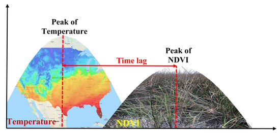
1. Introduction
The spatial extent and composition of coastal wetlands (CWs) varies in response to hydrologic and meteorological conditions (e.g., precipitation and wind) and extreme events (e.g., droughts and floods). These variations represent a major source of CW alteration on the global, regional, and local scale [1,2,3,4,5]. Knowledge of CW dynamics across scales is important as these wetlands provide a variety of ecosystem services such as habitat [6], protection from storm surges [7,8], water quality enhancement by nutrient uptake and filtration, carbon sequestration, and commercial and recreational fishing. CWs also provide other important ecosystem services such as erosion control, local water storage improvement [9], climate regulation and stabilization, and are a unique aesthetic landscape of cultural, historic, and spiritual relevance [7].
The characterization of both terrestrial wetland [10,11] and CW dynamics can be efficiently approached by using satellite remote sensing data that are available over wide and consistently sampled coverage areas. Satellite remote sensing can be particularly useful for monitoring long-term CW changes [12,13]. The normalized difference vegetation index (NDVI) is a vegetation index that is used to measure vegetation greenness and can be derived from several remote sensors. This index is sensitive to the green vegetation biomass as affected by the type of wetland and season [14]. It has been well correlated with wetland greenness, for example, in Apalachicola Bay of Florida [1,15]. Landsat NDVI is also regarded as a reliable indicator for wetland greenness change detection [16]. Furthermore, NDVI derived from Landsat has the most comprehensive spatial and temporal coverage along with reasonable resolution when compared to other publicly available satellite imagery. Landsat-5 has been collecting valuable information since 1984 and such a long-term record is unique among satellite remote sensing products.
Previous studies established that vegetation phenology in different parts of the world is a key indicator of climate–biosphere interactions [17,18,19]. Timing of phenology is linked to precipitation [17] and temperature [18,19], especially, in the northern high-latitudes. As the global hydro-meteorology changes as part of the climate, vegetation is adapting and simultaneously feeding back to the larger system [20,21].
The presence of feedback mechanisms between Earth’s coastal/terrestrial systems and hydro-meteorology, implies the presence of cross-correlation structures (interdependencies) and memory effects. Within this feedback structure, the concept of persistence, explained through the idea of scaling behavior of Fourier transformed hydro-meteorological signals [22,23], can be useful to discern the resilience of wetland vegetation. Persistence of a system refers to a phenomena that is controlled by positive feedback mechanisms, which tend to disrupt the stability properties of the system and make them vulnerable to external forces [24,25,26]. Since resilience of a system is the capability to respond to a disturbance by resisting damage and recovering quickly, ecosystem resilience can be studied by their persistence through time [27]. The quantification of memory and persistence in a signal requires long-term data and satellite remote sensing often fills this need. However, not all satellites provide long-term time series data and there is often missing information within the available time-frame. A methodical and repeatable framework for addressing this issue is therefore required to characterize vegetation dynamics at temporal scales ranging from seasonal to multi-decadal.
In this study, we use the time series of the NDVI and hydro-meteorological data from 1984 to 2015 for Apalachicola Bay, Florida. Spectral analysis of these data allows for the characterization of persistence in the signal, which in our case refers to the analysis of Fourier transformed NDVI and hydrometeorological signals. While previous studies focused on vegetation dynamics in terrestrial areas using conventional data and methods, CW dynamics using long-term remote sensing data and robust methodologies for the extraction of complex interaction related information is understudied. This study aims to partially fill that knowledge gap.
We quantified the time-lag between forcing (hydro-meteorological) and response (NDVI) signals for target coastal areas based on the National Oceanic and Atmospheric Administration (NOAA) Coastal Change Analysis Program (C-CAP) classification system. Most previous models estimated time-lag using linear correlation or cross-correlation between changes in two or more indices over time or used a time-lag defined a priori. This could lead to spurious or insufficient results due to the large variation in NDVI across both spatial and temporal scales, making previous assumptions unsuitable to be adopted globally or locally [2]. The influence of the varying growth periods of vegetation could affect the results as well. We minimized the limitations in a novel way by applying cross-spectral analysis over wetland vegetation and hydro-meteorological signals which allow determination of the similarities between the two signals as a function of frequency with the help of phase shift; and second by classifying CWs in the study area from C-CAP defined land cover classes; and third by extracting time-lags directly from cross-spectral components. Thus, the novelty of the study lies in applying conventional power-spectra and cross-spectral analysis to remote sensing signals and hydro-meteorological signals to extract any possible time-lag between the signals.
The aim of the study was to (i) understand and quantify prevailing variability in persistent behavior among different CW vegetation classes; (ii) characterize the spatio-temporal sensitivity of CWs to hydro-meteorological signals under various frequency domains; and (iii) assess the spatial difference in time-lag between forcing (hydro-meteorological) and response (NDVI) signals.
2. Data and Methods
2.1. Site Description and Coastal Wetlands Classification
The setting for this study was Apalachicola Bay in the Florida Panhandle, with the specific study area indicated by the red boundary in Figure 1a. CWs have been classified by C-CAP along the eastern seaboard and Gulf coasts of the United States [28]. Figure 1b depicts the type and locations of CWs in the study area. The specific wetland classes investigated were: palustrine-forested wetlands (PFW): 54.1%; palustrine emergent wetlands (PEW): 7.9%; palustrine scrub and emergent wetlands (PSEW): 11.7%; and estuarine emergent wetlands (EEW): 6.48%. Other wetland classes such as estuarine forested wetland and estuarine scrub/shrub wetland were uncommon (<1%) in the study area. A total of 19.6% of the study area was comprised of land uses other than wetlands, including developed area, agricultural use, and bare land.
We selected six locations (Figure 1a) inside the study area to represent the dominant wetland types. The spatial variability of CWs includes PFW at two locations: Lake Wimico and Apalachicola River; EEW at two locations: lower Apalachicola River and St. Vincent Island; PSEW at one location: Eastern Apalachicola; and PEW at one location: South of Lake Wimico.
2.2. Forcing and Response Signals
Level-2 surface reflectance data from Landsat-5, Landsat-7, and Landsat-8 were acquired between 1984 and 2015 from United States Geological Survey (USGS) Earth Resources Observation and Science Center archive to calculate NDVI. Level-2 surface reflectance products are atmospherically corrected. After image acquisition, all georeferenced images were clipped to the spatial extent of the study area. Resampling and projection using WGS1984 UTM Zone 16N was implemented using ArcGIS. NDVI was calculated as the normalized ratio of red (R) and near-infrared (NIR) reflectance of a sensor system and generally characterized the greenness of wetland vegetation. It is commonly expressed as:
In this paper, we used the processed NDVI dataset developed by Tahsin et al. for this study area [15]. The NDVI data time series are similar except for the four ecosystem classifications across the six locations used herein. However, the complete NDVI time series data were limited by clouds and other effects. For instance, only 252 months of data were usable out of the 384 months of the study time period [15,29]. Since NDVI is released as a 16-day composite, when two images were available for a given month the one with less cloud coverage was selected. The majority of the images were collected from Landsat-5 since it was the only source from 1984 to 2013. Landsat-7 data were avoided when any other version of Landsat data was available as it has a known issue with the scan line corrector (SLC) in the Landsat Enhanced Thematic Mapper Plus (ETM+) sensor that failed permanently in 2003 [53]. The remainder of the data came from Landsat-8. In order to overcome the remaining data gaps in the time series [29], a Saviszky–Golay filter was used for both interpolating missing data and discounting spurious low NDVI values [30,31,32]. To compare the performance of the filter, a goodness of fit test between the original NDVI and some known but reconstructed NDVI data using the Saviltzky–Golay filter was conducted. Coefficient of determination, F-statistics, and p-value were computed. The R-square value (0.88) showed a good fit which explained 88% of the variation in the reconstructed NDVI by the original NDVI data around its mean. Also, both the F-statistics and p-value were found to be less than 0.05, suggesting that the filter was effective towards reconstructing the time series.
For heavily vegetated areas, NIR reflectance was greater than red reflectance due to the tendency of chlorophyll to absorb red light. In those areas, NDVI values were expected to be greater than 0 [15,33]. The wetland classification was superimposed onto the wetland NDVI values to set NDVI boundaries for different CW classes.
Water level, precipitation, temperature, and wind speed data were collected for the same spatial region and time period. Water level data were collected from NOAA/National Ocean Service (NOS) coastal gage station (Station ID: 8728690) located at Apalachicola, FL. Precipitation, temperature, and wind speed data were collected from Automated Surface Observing System (ASOS) stations located at the airports in the United States and maintained by Iowa State University, Iowa Environmental Mesonet. The AAF Apalachicola Muni ASOS station, located in the south of the Apalachicola River inside the study area was used for analysis in the study.
2.3. Methodology
2.3.1. Power Spectral Density and Scaling Behavior in the Frequency Domain
Power spectral density (PSD) is a measure of the frequency response to the variation in a signal. In general, PSD analysis provides a standard method to identify correlation features in time series fluctuations and describes how the energy in a signal is distributed across various frequencies. The PSD of a discrete signal can be computed as the average of the Fourier transform magnitude squared, over a large time interval and expressed as follows:
where is the discrete Fourier transform of , is its complex conjugate, and is the wavenumber [34,35,36,37,38,39].
We analyzed the scaling behavior of the PSD which was determined to be a power-law dependence of the spectrum on the frequency in the following form:
Here β is the power-law exponent of the PSD. A robust estimation of the scaling exponent β can be achieved by computing the slope of the linear regression fitted to the estimated PSD plotted on log-log scales [40]. The strength of these scaling exponents provides useful information about the inherent memory of the system [26,41,42]. Witt and Malamud [26] found PSD analysis to be a more accurate method to quantify persistence of self-affine time series than other empirical methods such as Hurst rescaled range (R/S) analysis, detrended fluctuation analysis, and semi-variogram analysis. The basic feature of a self-affine time series is that the PSD of the time series has a power-law dependence on frequency and as a result exhibits long-range persistent behavior [43,44]. In other words, a time series is self-affine if it exhibits statistical self-similarity (i.e., invariance under suitable scaling of time or space scale) and has the same statistical properties [45] when the two axes are scaled differently. A steeper PSD indicates a higher persistence (or high vulnerability) which characterizes stability or instability in the concerned ecosystem. In more general cases of long-range persistence, β ~0 implies that the temporal fluctuations are purely random and are characterized by the uncorrelated sample, typically white noise processes; is known as a pink or flicker noise [42,43]. Pink noise is a statistically reliable departure from white noise in the direction of persistence [46]. is known as brown noise (or Brownian motion), however its increments are uncorrelated and result in white noise with = 0. Both pink and brown noise correspond to persistent behavior and indicate the presence of a positive feedback mechanism.
2.3.2. Cross-Spectrum and Time-Lag Analysis Between Signals in the Frequency Domain
Cross-spectrum analysis relates the variance of two signals. The cross power spectral density (CPSD) is computed using a real valued PSD estimate of time series defined as (ω) and the complex conjugate of the PSD estimate of time series defined as (ω) in the frequency domain (ω), and is given by:
The real component of the CPSD is defined as the co-spectrum, Co, whereas the imaginary component is defined as the quadrature spectrum, Q. Equation (4) can thus be re-written as:
The phase spectrum estimate is bounded between −π and π and is the phase difference at each frequency between and . It can be calculated either in radians or in degrees from the real and imaginary components of the CPSD as follows:
Finally, the time-lag can be obtained from the phase spectrum as:
where is the phase in degrees and is the linear frequency [3].
3. Results
The PSD of CW NDVIs has been studied extensively and is a commonly used tool to measure the distribution of energy in the signals across frequencies or wavenumbers. To understand the characteristics of the original CW NDVI signals, the NDVI time series for the six selected locations from 1984 to 2015 (sampled monthly) were analyzed and are shown in Figure 2a.
The three black-dashed boxes in the time series highlight the dynamic behavior of the NDVIs ranging from approximately 0.1 to 0.9 and are shown in greater detail in Figure 2b (1985 to 1987), Figure 2c (1995 to 1996), and Figure 2e (2004 to 2006), which were marked by several extreme events including various minor and major hurricanes, droughts, and floods [47]. The black solid box highlights less dynamic NDVIs ranging from approximately 0.4 to 0.9 (Figure 2d; 2001 to 2002), where there were no reported extreme events. However, the NDVI for PFW still had a distinct peak and drop during this but varied little for EEW, PEW, and PSEW. Therefore, these time series hinted at the disparate response among PFW, PSEW, PEW, and EEW.
To further investigate the disparate behavior among different wetland types, we identified peak greenness and explored periodic trends using PSD analysis. Figure 3 shows the averaged PSD of NDVIs at six locations in Apalachicola Bay (see Figure 1 for location). Visual observation suggests that the PSDs, which were plotted in log-log scale, were not flat (slope ≠ 0) for the analyzed frequency scale. This indicated that the wetland dynamics were not characterized by purely random and uncorrelated temporal fluctuations but instead contained correlated time-structure and memory phenomena.
Figure 3a,b shows two different modality behaviors with distinct annual (frequency peaks at f = 0.085 (month−1)) and semi-annual peaks (frequency peaks at f = 0.1693 (month−1)). Modality indicates the periodicity of the vegetation. Generally, multi-modality occurs in places with double cropping, or with vegetation that is highly responsive to bi-modal temperature and/or precipitation regimes, or with diverse land-cover types [48]. In our case, there were two peaks of greenness for PFW occurring at different times. This was mainly due to the heterogeneity of the PFW, which consists mostly of woody vegetation both in tidal and non-tidal wetlands. Characteristic species are Tupelo (Nyssa), Cottonwoods (Populus deltoids) and Bald Cypress (Taodium distichum) [49].
However, for the other four sites (PSEW, PEW, and EEW), shown in Figure 3c–f, there was a unimodal seasonal NDVI cycle. This peak (f = 0.085 (month−1)) indicated a strong annual component of the NDVI fluctuations. An early spring soil moisture peak supporting initial springtime plant emergence was observed for PSEW, PEW, and EEW in Apalachicola Bay, followed by 3–4 months of gradual plant growth until the summertime rain provided adequate moisture for the rapidly established NDVI peak.
The results also indicated two scaling regimes in the PSDs of the wetlands associated with annual and decadal scales. In the annual frequency domain, the slopes were steeper for the PSD of PFW NDVI compared to the slope for the PSDs of PSEW, PEW, and EEW NDVIs. Coastal forests (here PFW) were also found to be more persistent in a previous study in southern Italy [22]. In this study, the persistence reversal was observed at the decadal frequency where the NDVI values for the PSEW, PEW, and EEW were more persistent than PFW. Figure 2d graphically explains the dynamic nature of PFW annually where NDVI dropped sharply (from 0.9 to 0.4) while the NDVI for the other wetland categories fluctuated within a much narrower range (from 0.6 to 0.4). At the decadal scale, PSEW, PEW, and EEW had larger persistence in NDVI values compared to PFW which indicates a more unstable character with respect to external perturbations.
Figure 4 shows the PSDs of the four hydro-meteorological signals: water level, precipitation, temperature, and wind in Apalachicola Bay, which we refer to as forcing mechanisms. For visual comparison, we vertically shifted the PSDs on the log-log plot. Figure 4 clearly shows a distinct annual peak for water level and temperature similar to what was observed for the NDVI for the different wetland types (Figure 3). The major peak suggests an interdependence between the vegetation dynamics of all wetland types and the annual water level and temperature fluctuations. The figure also exhibits steeper spectral slope for water level and precipitation, which indicates that the temporal fluctuations of water level and precipitation were persistent and related by memory. On the other hand, the PSD for temperature and wind were flat suggesting uncorrelated behavior of fluctuations across spatial and temporal scales.
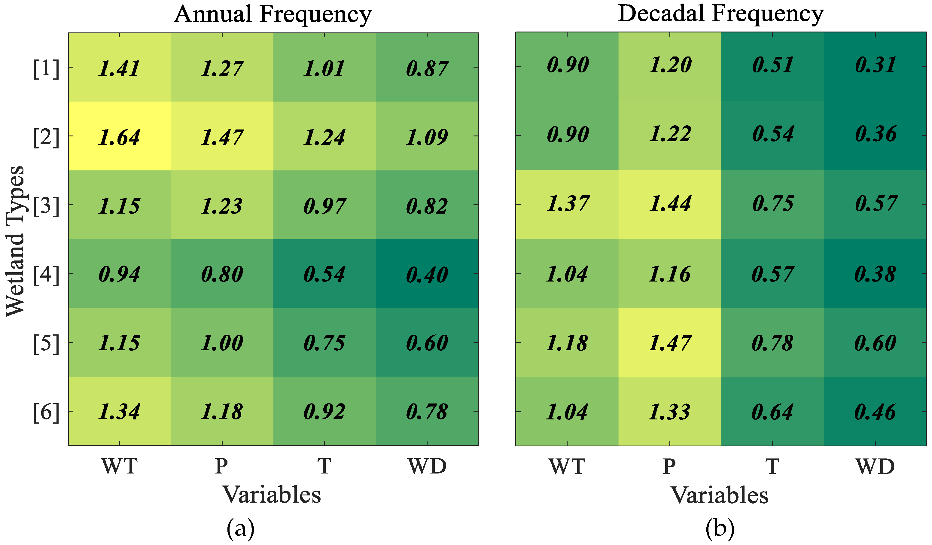
Figure 5 shows a heat-map of cross-spectral slope obtained from the CPSD analysis between each of the CW NDVI values and hydro-meteorological signals at the annual (Figure 5a) and decadal (Figure 5b) scales.
Recall that CPSD refers to the comparison between two signals as a function of frequency with the help of a phase shift while PSD helps interpret how the energy in an individual signal is distributed across various frequencies. Here, the slope of the CPSD serves as a measure of the influence of hydro-meteorological signal onto wetland types. The warmer colors indicate a steeper slope, which is suggestive of a more persistent, and thus less resilient [50,51] relation between the forcing and response signal. Figure 5 shows the largest CPSD slopes for water level and precipitation for all wetland types in both annual and decadal scales indicating that wetlands responded more to the changes in water level and precipitation across all scales compared to wind and temperature. Figure 5 also depicts a reverse scenario for the wetland types in two different frequency domains. While annually PFW responded promptly to the change in hydro-meteorological forcing; PFW responded less for decadal scale with hydro-meteorological mechanisms. In summary, inland wetlands exhibited more vulnerability at the annual scale while in the decadal scale they were less vulnerable. The PFW, PSEW, PEW, and EEW persistence character with respect to hydro-meteorological signals provides valuable information that can be used in supporting local environmental protection agencies. Such information can be used both for the identification of most vulnerable areas in short- or long-term scales and for most effective protection strategies.
Components of CPSD analysis (i.e., percentage of amplitude with the major peak, phase lag, and corresponding time-lag) are shown in Table 1. Major peaks in the amplitude spectra were identified by using a threshold quantified using a smoothed z-score algorithm [52,53,54]. The algorithm is based on the principle of dispersion and is robust as it builds a separate moving mean and deviation so that the signals themselves do not pollute the threshold [53]. Peak or high amplitude indicates a strong correlation between response and forcing signal at that frequency. While there are clear major peaks for temperature and water level, there were none for precipitation and wind. Precipitation had a minor peak for PEW at location 4 and wind had two minor peaks for PFW at locations 1 and 2 and one minor peak for PEW at location 4 (see Figure 1a for locations).
The major peak indicated that annually both periodic components of NDVI time series and temperature time series are correlated. The phase lag between the annual components of CW NDVIs and temperature ranged from approximately 24° to 81° (i.e., 0.8 month to 2.7 months). Our results suggest that the CW NDVI responded with a longer delay of maximum 2.7 months with temperature whereas, it responded with a shorter delay of maximum 2.2 months with water level. The time-lag was obtained using Equation (7) from the mean phase spectrum over frequencies within a range of +/−1 month.
4. Discussion
The study quantifies the CW NDVIs discrepancy through the conventional power spectral density and infers these CW NDVIs discrepancies by cross-spectral analysis with four hydro-meteorological signals (temperature, water level, wind, precipitation). A novel method has been adopted to assess the causal relationship between CW NDVI values and the time series of each hydro-meteorological signal one at a time. The method finally estimates the time-lag for all significant cross-spectral components.
Power spectral analysis shows very similar dynamical behavior among PSEW, PEW, and EEW NDVI values while PFW NDVI values show discrepancy from them. Two different modalities in PFW indicate two greenness peaks where, the main greenness peak was associated with the spring season, and the second peak was likely due to the larger availability of fresh water during the main precipitation season in the months of October and November. This finding is consistent with previous studies for both forested and scrub wetlands in the Mediterranean ecosystems of southern Italy and north American monsoon region [22,55,56]. However, for the other four sites (PSEW, PEW, and EEW), there was a unimodal seasonal NDVI cycle. This type of unimodal greenness is also found at south-west American regions, for example Utah/Colorado sites and Audubon but varied little regarding the NDVI cycle, where springtime snowmelt and an initial precipitation peak support springtime plant emergence; the plants keep growing gradually for the next 3-4 months and NDVI peaks in summertime [57].
Two scaling regimes—annual and decadal—were found in the PSDs of the wetlands. The finding was similar to previous findings where scrub wetlands (here PSEW) were found to be less persistent [58], and emergent wetlands (here PEW and EEW) were found to be more salt tolerant [59]. Coastal forests (here PFW) were also found to be more persistent in a previous study in southern Italy [22].
A striking feature of the results is the persistent reversal where the NDVI values for the PSEW, PEW, and EEW were more persistent than PFW in annual frequency. On the other hand, the NDVI values for the PSEW, PEW, and EEW were less persistent than PFW in decadal frequency. Hurricanes, storm surges or other hydrologic events impact the coastal areas over a relatively sudden and short time span and since PSEW, PEW, and EEW are generally located closer to the coast than PFW, they were impacted first and more severely.
The four hydro-meteorological signals: water level, precipitation, temperature, and wind in Apalachicola Bay, played an important role in the CW NDVIs dynamics. Results found an interdependence between the vegetation dynamics of all wetland types and the annual water level and temperature fluctuations. While annually PFWs responded promptly to the change in hydro-meteorological forcing, PFW responded less in decadal scale with hydro-meteorological mechanisms.
5. Summary and Conclusions
This study aimed to understand the dynamic nature of four types of coastal wetlands available in the study area by analyzing the interaction between the hydro-meteorological mechanisms (i.e., water level, precipitation, temperature, wind) that force these dynamics and the corresponding response in the CW NDVI value. The study also sought to understand the temporal lag between the response and forcing signals. The data used were Landsat-derived NDVIs, airport and tide station hydro-meteorological data, and an established wetland classification system. A series of empirical methods were implemented to analyze the time series under different situations.
The NDVI exhibited annual periodicity which appeared to be regulated primarily by temperature and water level. Cross-spectral analysis found a time-lag of 0.8 months to 2.7 months between temperature and NDVI and 0.9 months to 2.2 months between water level and NDVI. The characterization of the persistent behavior across a range of spatial and temporal scales and subsequent understanding that coastal wetland dynamics are mostly driven by water level and precipitation indicated that the severity of droughts, floods, and storm surges will be a driving factor in the future sustainability of coastal wetland ecosystems. For long-term projections of coastal wetland dynamics, we recommend that extreme hydrologic events (e.g., floods and hurricanes) be incorporated into the model at approximately decadal intervals and that wetland responses to temperature and storm surge events be lagged in time by the values indicated above.
Also, based on spectral analysis, on an annual scale, PFW (inland locations) were found to be less resilient to external forcing compared to PSEW, PEW, and EEW (coastal locations). However, at the decadal-scale, inland locations were more resilient (i.e., less vulnerable) than coastal locations. At the decadal time scale, CW losses can be severe with large swaths of CWs transitioning into unconsolidated shoreline. The regular extreme hydrologic events shaped the composition of the study area wetland types and we found the wetland dynamics to be driven primarily by water level and precipitation. The findings support the key role of water availability and precipitation in maintaining the CW dynamics around Apalachicola Bay. However, coastal wetlands also appear to play a protective role for inland locations, therefore efforts to restore and preserve estuarine wetlands will likely have a positive impact on the productivity and resilience of palustrine systems upriver.
Author Contributions
S.T. collected and processed the data, developed and integrated the code, and wrote the paper under the supervision of S.C.M. and A.S. A.S. planned and designed the work. S.C.M. guided the analysis and reviewed the paper. All authors have read and agreed to the published version of the manuscript.
Funding
This research was funded in part under award NA16NOS4780208 from the National Oceanic and Atmospheric Administration (NOAA) Ecological Effects of Sea Level Rise (EESLR) Program. A.S. acknowledges the partial support from the donors of the American Chemical Society. Article processing charges were provided in part by the UCF College of Graduate Studies Open Access Publishing Fund.
Acknowledgments
The data presented in this paper are publicly available and can be downloaded from https://earthexplorer.usgs.gov; https://waterdata.usgs.gov; https://mesonet.agron.iastate.edu.
Conflicts of Interest
The authors declare no conflicts of interest.
References
- La Cecilia, D.; Toffolon, M.; Woodcock, C.E.; Fagherazzi, S. Interactions between river stage and wetland vegetation detected with a Seasonality Index derived from LANDSAT images in the Apalachicola delta, Florida. Adv. Water Resour. 2016, 89, 10–23. [Google Scholar] [CrossRef] [Green Version]
- Clinton, N.; Yu, L.; Fu, H.; He, C.; Gong, P. Global-scale associations of vegetation phenology with rainfall and temperature at a high spatio-temporal resolution. Remote Sens. 2014, 6, 7320–7338. [Google Scholar] [CrossRef] [Green Version]
- Van Hoek, M.; Jia, L.; Zhou, J.; Zheng, C.; Menenti, M. Early drought detection by spectral analysis of satellite time series of precipitation and Normalized Difference Vegetation Index (NDVI). Remote Sens. 2016, 8, 422. [Google Scholar] [CrossRef] [Green Version]
- Bilskie, M.V.; Hagen, S.C.; Alizad, K.; Medeiros, S.C.; Passeri, D.L.; Needham, H.F.; Cox, A. Dynamic simulation and numerical analysis of hurricane storm surge under sea level rise with geomorphologic changes along the northern Gulf of Mexico. Earth’s Future 2016, 4, 177–193. [Google Scholar] [CrossRef] [Green Version]
- Passeri, D.L.; Hagen, S.C.; Plant, N.G.; Bilskie, M.V.; Medeiros, S.C.; Alizad, K. Tidal hydrodynamics under future sea level rise and coastal morphology in the Northern Gulf of Mexico. Earth’s Future 2016, 4, 159–176. [Google Scholar] [CrossRef] [Green Version]
- Sivaperuman, C.; Venkatraman, C. Marine Faunal Diversity in India; Academic Press: Cambridge, MA, USA, 2015. [Google Scholar] [CrossRef]
- Barbier, E. Valuing ecosystem services for coastal wetland protection and restoration: Progress and challenges. Resources 2013, 2, 213–230. [Google Scholar] [CrossRef] [Green Version]
- Wamsley, T.V.; Cialone, M.A.; Smith, J.M.; Atkinson, J.H.; Rosati, J.D. The potential of wetlands in reducing storm surge. Ocean Eng. 2010, 37, 59–68. [Google Scholar] [CrossRef]
- Wong, C.P.; Jiang, B.; Bohn, T.J.; Lee, K.N.; Lettenmaier, D.P.; Ma, D.; Ouyang, Z. Lake and wetland ecosystem services measuring water storage and local climate regulation. Water Resour. Res. 2017, 53, 3197–3223. [Google Scholar] [CrossRef] [Green Version]
- Papa, F.; Prigent, C.; Durand, F.; Rossow, W.B. Wetland dynamics using a suite of satellite observations: A case study of application and evaluation for the Indian Subcontinent. Geophys. Res. Lett. 2006, 33. [Google Scholar] [CrossRef]
- Tadesse, T.; Demisse, G.B.; Zaitchik, B.; Dinku, T. Satellite-based hybrid drought monitoring tool for prediction of vegetation condition in Eastern Africa: A case study for Ethiopia. Water Resour. Res. 2014, 50, 2176–2190. [Google Scholar] [CrossRef]
- Rodgers, J.C.; Murrah, A.W.; Cooke, W.H. The impact of hurricane katrina on the coastal vegetation of the weeks bay reserve, alabama from NDVI data. Estuaries Coasts 2009, 32, 496–507. [Google Scholar] [CrossRef]
- Steyer, G.D.; Couvillion, B.R.; Barras, J.A. Monitoring vegetation response to episodic disturbance events by using multitemporal vegetation indices. J. Coast. Res. 2013, 63, 118–130. [Google Scholar] [CrossRef]
- Guo, M.; Li, J.; Sheng, C.; Xu, J.; Wu, L. A review of wetland remote sensing. Sensors 2017, 17, 777. [Google Scholar] [CrossRef] [PubMed] [Green Version]
- Tahsin, S.; Medeiros, S.C.; Singh, A. Resilience of coastal wetlands to extreme hydrologic events in Apalachicola Bay. Geophys. Res. Lett. 2016, 43, 7529–7537. [Google Scholar] [CrossRef]
- Kayastha, N.; Thomas, V.; Galbraith, J.; Banskota, A. Monitoring wetland change using inter-annual landsat time-series data. Wetlands 2012, 32, 1149–1162. [Google Scholar] [CrossRef]
- Maignan, F.; Bréon, F.M.; Bacour, C.; Demarty, J.; Poirson, A. Interannual vegetation phenology estimates from global AVHRR measurements. Comparison with in situ data and applications. Remote Sens. Environ. 2008, 112, 496–505. [Google Scholar] [CrossRef]
- Zhou, L.; Tucker, C.J.; Kaufmann, R.K.; Slayback, D.; Shabanov, N.V.; Myneni, R.B. Variations in northern vegetation activity inferred from satellite data of vegetation index during 1981 to 1999. J. Geophys. Res. Atmos. 2001, 106, 20069–20083. [Google Scholar] [CrossRef]
- Myneni, R.B.; Keeling, C.D.; Tucker, C.J.; Asrar, G.; Nemani, R.R. Increased plant growth in the northern high latitudes from 1981 to 1991. Nature 1997, 386, 698–702. [Google Scholar] [CrossRef]
- Kirilenko, A.P.; Sedjo, R.A. Climate change impacts on forestry. Proc. Natl. Acad. Sci. USA 2007, 104, 19697–19702. [Google Scholar] [CrossRef] [Green Version]
- Foley, J.A.; Kutzbach, J.E.; Coe, M.T.; Levis, S. Feedbacks between climate and boreal forests during the Holocene epoch. Nature 1994, 371, 52. [Google Scholar] [CrossRef]
- Telesca, L.; Lasaponara, R. Quantifying intra-annual persistent behaviour in SPOT-VEGETATION NDVI data for Mediterranean ecosystems of southern Italy. Remote Sens. Environ. 2006, 101, 95–103. [Google Scholar] [CrossRef]
- Feder, J. Fractals; Springer: Berlin/Heidelberg, Germany, 1988; ISBN1 978-1-4899-2126-0. ISBN2 978-1-4899-2124-6. [Google Scholar] [CrossRef]
- Zheng, H.; Song, W.; Satoh, K. Detecting long-range correlations in fire sequences with Detrended fluctuation analysis. Phys. A Stat. Mech. Its Appl. 2010, 389, 837–842. [Google Scholar] [CrossRef]
- Maktav, D. Remote sensing for a changing Europe. In Proceedings of the 28th Symposium of the European Association of Remote Sensing Laboratories, Istanbul, Turkey, 2–5 June 2008; IOS Press: Amsterdam, The Netherlands, 2009. ISBN 978-1-58603-986-8. [Google Scholar]
- Witt, A.; Malamud, B.D. Quantification of long-range persistence in geophysical time series: Conventional and benchmark-based improvement techniques. Surv. Geophys. 2013, 34, 541–651. [Google Scholar] [CrossRef] [Green Version]
- Switzer, T.S.; Winner, B.L.; Dunham, N.M.; Whittington, J.A.; Thomas, M. Influence of sequential hurricanes on nekton communities in a southeast Florida estuary: Short-term effects in the context of historical variations in freshwater inflow. Estuaries Coasts 2006, 29, 1011–1018. [Google Scholar] [CrossRef]
- Ramsey, E.W., III; Nelson, G.A.; Sapkota, S.K. Coastal change analysis program implemented in Louisiana. J. Coast. Res. 2001, 17, 53–71. [Google Scholar]
- Tahsin, S.; Medeiros, S.C.; Hooshyar, M.; Singh, A. Optical cloud pixel recovery via machine learning. Remote Sens. 2017, 9, 527. [Google Scholar] [CrossRef] [Green Version]
- Savitzky, A.; Golay, M.J.E. Smoothing and differentiation of data by simplified least squares procedures. Anal. Chem. 1964, 36, 1627–1639. [Google Scholar] [CrossRef]
- Chen, J.; Jönsson, P.; Tamura, M.; Gu, Z.; Matsushita, B.; Eklundh, L. A simple method for reconstructing a high-quality NDVI time-series data set based on the Savitzky-Golay filter. Remote Sens. Environ. 2004, 91, 332–344. [Google Scholar] [CrossRef]
- Luo, J.; Ying, K.; Bai, J. Savitzky-Golay smoothing and differentiation filter for even number data. Signal Process. 2005, 85, 1429–1434. [Google Scholar] [CrossRef]
- Tahsin, S.; Medeiros, S.C.; Singh, A. Assessing coastal wetland resiliency to extreme events using remote sensing. Remote Sens. 2018, 10, 1390. [Google Scholar] [CrossRef] [Green Version]
- Singh, A.; Guala, M.; Lanzoni, S.; Foufoula-Georgiou, E. Bedform effect on the reorganization of surface and subsurface grain size distribution in gravel bedded channels. Acta Geophys. 2012, 60, 1607–1638. [Google Scholar] [CrossRef]
- Stoica, P.; Randolph, L.M. Introduction to Spectral Analysis; Prentice Hall: Upper Saddle River, NJ, USA, 1997; Volume 1. [Google Scholar]
- Stull, R.B. An Introduction to Boundary Layer Meteorology; Springer Science+Business Media: Medford, MA, USA, 2012; Volume 13. [Google Scholar]
- Gardner, W.A. Statistical spectral analysis: A nonprobabilistic theory. Technometrics 1986, 34, 109–110. [Google Scholar] [CrossRef] [Green Version]
- Keylock, C.J.; Singh, A.; Foufoula-Georgiou, E. The complexity of gravel bed river topography examined with gradual wavelet reconstruction. J. Geophys. Res. Earth Surf. 2014, 119, 682–700. [Google Scholar] [CrossRef] [Green Version]
- Singh, A.; Lanzoni, S.; Wilcock, P.R.; Foufoula-Georgiou, E. Multiscale statistical characterization of migrating bed forms in gravel and sand bed rivers. Water Resour. Res. 2011, 47. [Google Scholar] [CrossRef] [Green Version]
- Pilgram, B.; Kaplan, D.T. A comparison of estimators for 1/f noise. Phys. D Nonlinear Phenom. 1998, 114, 108–122. [Google Scholar] [CrossRef]
- Hansen, A.; Singh, A. High-frequency sensor data reveal across-scale nitrate dynamics in response to hydrology and biogeochemistry in intensively managed agricultural basins. J. Geophys. Res. Biogeosci. 2018, 123, 2168–2182. [Google Scholar] [CrossRef]
- Bak, P.; Tang, C.; Wiesenfeld, K. Self-organized criticality: An explanation of the 1/f noise. Phys. Rev. Lett. 1987, 59, 381. [Google Scholar] [CrossRef]
- Mandelbrot, B.B.; Ness, V. Fractional Brownian motions, fractional noises and applications. SIAM Rev. 1968, 10, 422–437. [Google Scholar] [CrossRef]
- Malamud, B.D.; Turcotte, D.L. Self-affine time series: I. Generation and analyses. Adv. Geophys. 1999, 40, 1–90. [Google Scholar] [CrossRef]
- Mandelbrot, B.B. The fractal geometry of nature. Am. Math. Mon. 1984, 91, 594–598. [Google Scholar] [CrossRef]
- Holden, G.J. Gauging the fractal dimension of response times from fractal geometry. In Contemporary Nonlinear Methods for Behavioral Scientists: A Webbook Tutorial; 2005. Available online: WWW.NSF.GOV/SBE/BCS/PAC/NMBS/NMBS.J (accessed on 16 September 2019).
- Hurricane Research Division. Chronological List of All Hurricanes which Affected the Continental United States: 1851–2012. Available online: https://web.archive.org/web/20140210221648/http://www.aoml.noaa.gov/hrd/hurdat/All_U.S._Hurricanes.html (accessed on 23 October 2018).
- Yang, L.; Homer, C.; Hegge, K.; Huang, C.; Wylie, B.; Reed, B. A Landsat 7 scene selection strategy for a National Land Cover Database. In Proceedings of the IEEE 2001 International Geoscience and Remote Sensing Symposium (Catalogue No. 01CH37217), Sydney, Ausralia, 9–13 July 2001; Volume 3, pp. 1123–1125. [Google Scholar]
- Conner, W.; Buford, M.A. Southern Forested Wetlands; Messina, M.G., Conner, W.H., Eds.; CRC Press LLC: Boca Raton, FL, USA; Boston, MA, USA; New York, NY, USA; Washington, DC, USA; London, UK, 1998; ISBN l-56670-228-3. [Google Scholar]
- Holling, C.S. Resilience and stability of ecological systems. Annu. Rev. Ecol. Syst. 1973, 4, 1–23. [Google Scholar] [CrossRef] [Green Version]
- Gunderson, L.H. Ecological resilience—In theory and application. Annu. Rev. Ecol. Syst. 2002, 31, 425–439. [Google Scholar] [CrossRef] [Green Version]
- Perkins, P.; Heber, S. Identification of ribosome pause sites using a Z-score based peak detection algorithm. In Proceedings of the IEEE 8th International Conference on Computational Advances in Bio and Medical Sciences (ICCABS), Las Vegas, NV, USA, 18–20 October 2018; pp. 1–6, ISBN 978-1-5386-8520-4. [Google Scholar]
- Lo, O.; Buchanan, W.J.; Griffiths, P.; Macfarlane, R. Distance measurement methods for improved insider threat detection. Secur. Commun. Netw. 2018, 2018, 5906368. [Google Scholar] [CrossRef]
- Moore, J.; Goffin, P.; Meyer, M.; Lundrigan, P.; Patwari, N.; Sward, K.; Wiese, J. Managing in-home environments through sensing, annotating, and visualizing air quality data. Proc. ACM Interact. Mob. Wearable Ubiquitous Technol. 2018, 2, 128. [Google Scholar] [CrossRef] [Green Version]
- Lizárraga-Celaya, C.; Watts, C.J.; Rodríguez, J.C.; Garatuza-Payán, J.; Scott, R.L.; Sáiz-Hernández, J. Spatio-temporal variations in surface characteristics over the North American Monsoon region. J. Arid Environ. 2010, 74, 540–548. [Google Scholar] [CrossRef]
- Vivoni, E.R.; Moreno, H.A.; Mascaro, G.; Rodriguez, J.C.; Watts, C.J.; Garatuza-Payan, J.; Scott, R.L. Observed relation between evapotranspiration and soil moisture in the North American monsoon region. Geophys. Res. Lett. 2008, 35. [Google Scholar] [CrossRef] [Green Version]
- Notaro, M.; Liu, Z.; Gallimore, R.G.; Williams, J.W.; Gutzler, D.S.; Collins, S. Complex seasonal cycle of ecohydrology in the Southwest United States. J. Geophys. Res. Biogeosci. 2010, 115. [Google Scholar] [CrossRef]
- Dinerstein, E.; Weakley, A.; Noss, R.; Snodgrass, R.; Wolfe, K. Florida Sand Pine Scrub. Available online: https://www.worldwildlife.org/ecoregions/na0513 (accessed on 19 Feburary 2019).
- Adam, P. Saltmarsh Ecology; Cambridge University Press: Cambridge, UK, 1990; ISBN 0-521-24508-7. [Google Scholar]
Figure 1.
(a) Classes of wetlands in the Apalachicola Bay; (b) distinguishing wetland habitats in palustrine and estuarine wetlands. Coastal wetland (CW) ecosystem definitions based on National Oceanic and Atmospheric Administration (NOAA) Coastal Change Analysis Program (C-CAP). palustrine forested wetland (PFW); palustrine emergent wetland (PEW); estuarine emergent wetland (EEW); palustrine scrub/shrub; and palustrine emergent wetland (PSEW). Mean high water (MHW); mean sea level (MSL); low water (LW); Automated Surface Observing System (ASOS).
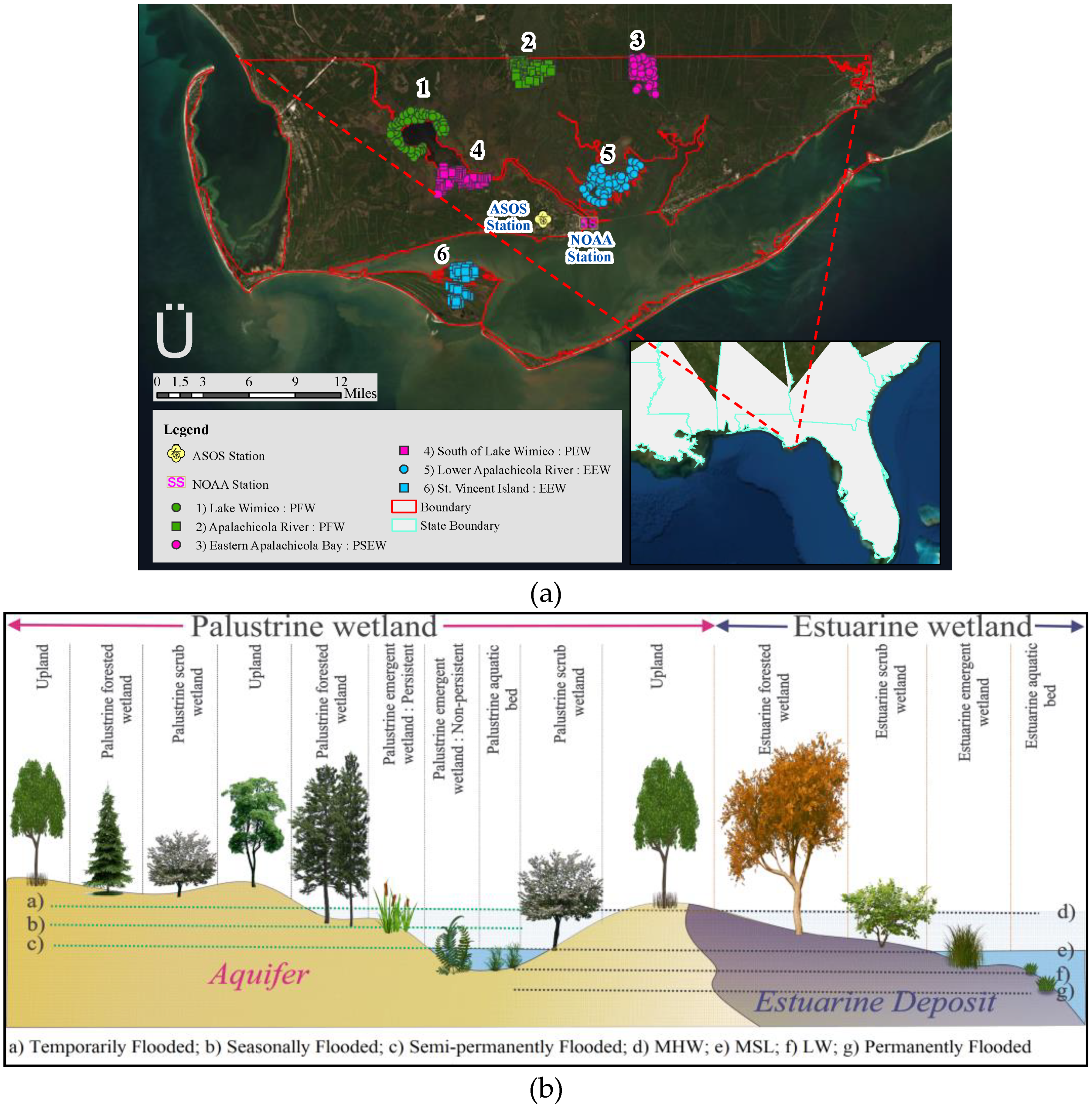
Figure 2.
(a–e) Normalized difference vegetation indices (NDVIs) at six spatially separated locations in Apalachicola Bay, Florida from 1984 to 2015. [1]–[6] in the legend indicate the locations of the wetlands (see Figure 1a).
Figure 2.
(a–e) Normalized difference vegetation indices (NDVIs) at six spatially separated locations in Apalachicola Bay, Florida from 1984 to 2015. [1]–[6] in the legend indicate the locations of the wetlands (see Figure 1a).
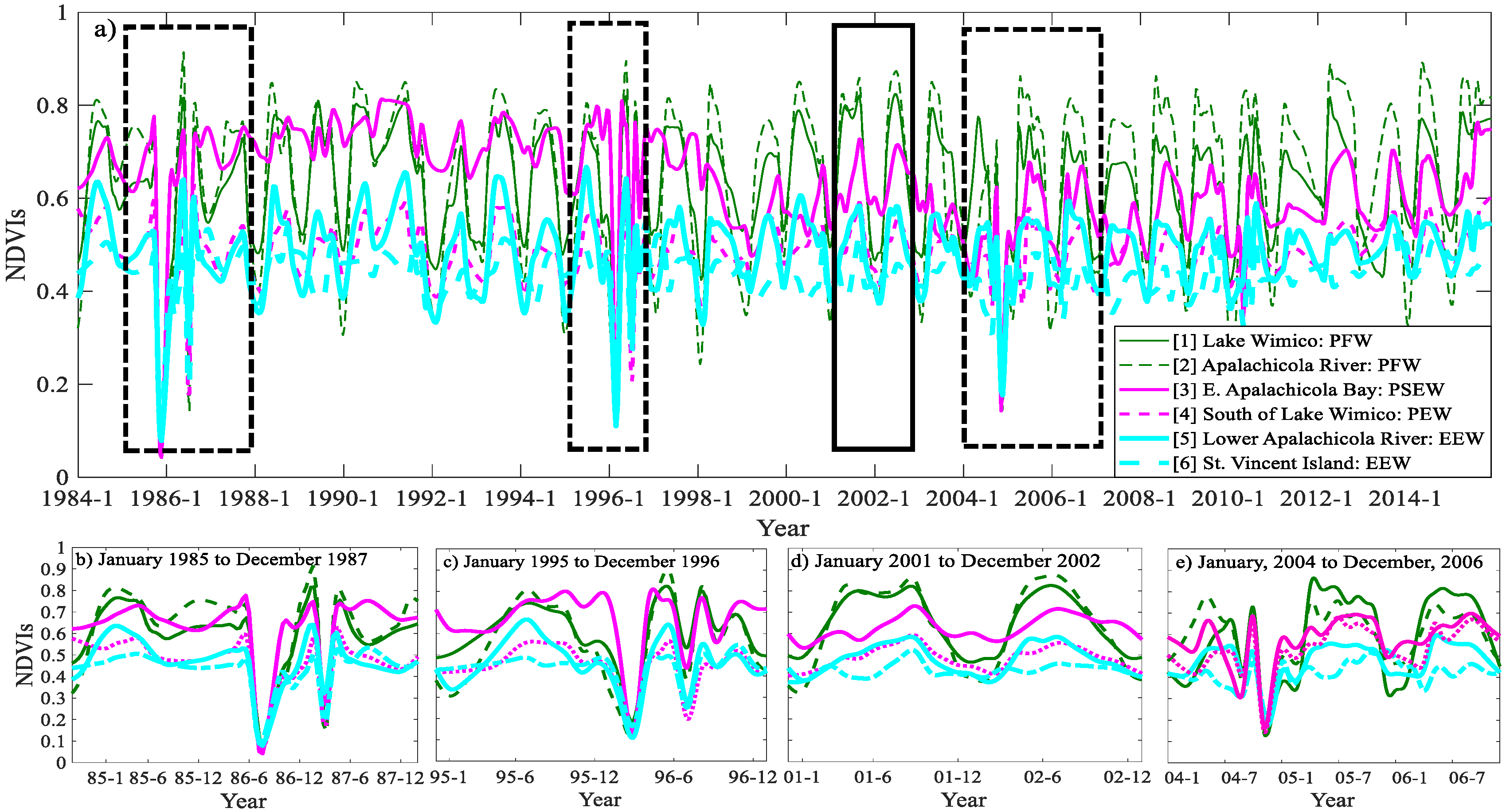
Figure 3.
(a–f) Power spectral density (PSD) of NDVIs at spatially separated wetland locations around Apalachicola Bay, Florida. For all locations, the PSDs were computed as an average of PSDs from 60 data points (pixels); the locations are shown in Figure 1.
Figure 3.
(a–f) Power spectral density (PSD) of NDVIs at spatially separated wetland locations around Apalachicola Bay, Florida. For all locations, the PSDs were computed as an average of PSDs from 60 data points (pixels); the locations are shown in Figure 1.
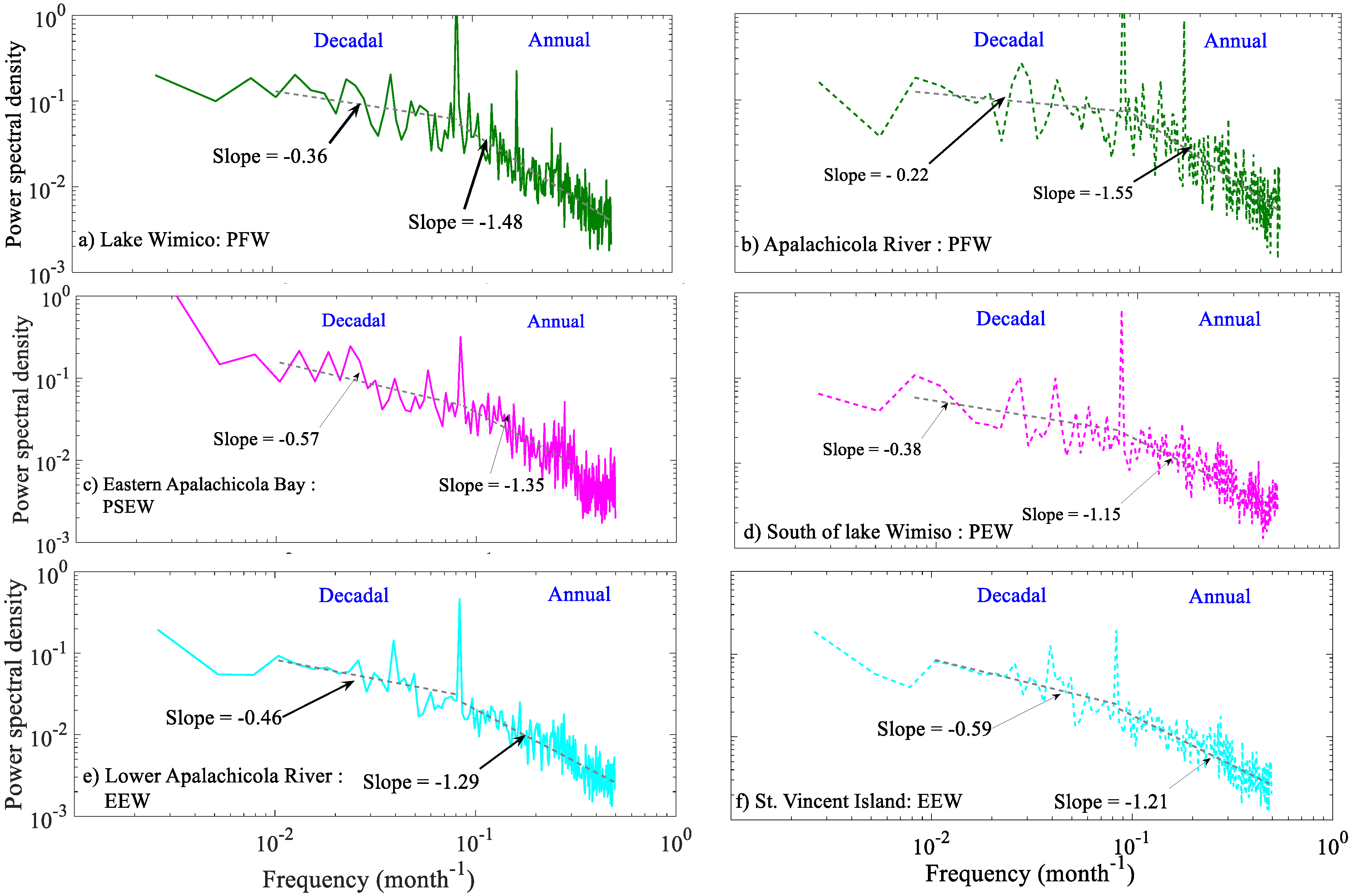
Figure 4.
Power spectral density (PSD) of water level, precipitation, temperature, and wind. The dashed linear lines represent the slopes of the annual and decadal frequency regimes.
Figure 4.
Power spectral density (PSD) of water level, precipitation, temperature, and wind. The dashed linear lines represent the slopes of the annual and decadal frequency regimes.

Figure 5.
(a,b) Heat-map of cross power spectral density (CPSD) slope between NDVI and four hydro-meteorological signals: water level (WT), precipitation (P), temperature (T), and wind (WD). Color bar shows the magnitude of the CPSD slope. [1]–[6] shows the locations of the different wetland types (see Figure 1a).

Table 1.
Summary of cross-spectral (CPSD) analysis between NDVI and different hydro-meteorological signals. Amplitude % was computed as the ratio of amplitude at the peak to the sum of amplitudes at all frequencies. Phase-lag and time-lag were computed using Equations (6) and (7), respectively. Major peak was computed using the smoothed z-score algorithm. In the last column, the square brackets [] represent frequencies corresponding to the % of amplitude.
| Cross Power Spectral Density (CPSD) Variables | (Major Peak) % of Amplitude at Annual Frequency | Phase-Lag (Degree) | Time-Lag (Months) | (Minor Peak) % of Amplitude at Other Frequencies |
|---|---|---|---|---|
| Wet 1 vs. temperature | 31.6 | 81.9 | 2.7 | 1.0 [Every 1.2 years] |
| Wet 2 vs. temperature | 39.5 | 62.3 | 2.1 | 0.7 [Every 8 years] |
| Wet 3 vs. temperature | 22.0 | 24.5 | 0.8 | No minor peak |
| Wet 4 vs. temperature | 32.6 | 32.0 | 1.1 | 0.5 [Every 8 years] |
| Wet 5 vs. temperature | 37.4 | 56.2 | 1.9 | No minor peak |
| Wet 6 vs. temperature | 16.7 | 50.8 | 1.7 | 1.0 [Every 6 years] |
| Wet 1 vs. water level | 11.2 | 66.0 | 2.2 | 2.3 [Every 5 years] |
| Wet 2 vs. water level | 19.1 | 46.6 | 1.6 | 2.3 [Every 8 years] |
| Wet 3 vs. water level | 16.1 | 39.7 | 1.3 | 2.1 [Every 1.6 years] |
| Wet 4 vs. water level | 15.7 | 26.3 | 0.9 | 1.6 [Every 5 years] |
| Wet 5 vs. water level | 17.5 | 46.6 | 1.6 | No minor peak |
| Wet 6 vs. water level | 14.1 | 41.8 | 1.4 | 1.4 [Every 2 years] |
| Wet 1 vs. wind | No major peak | N/A | N/A | 4.1 [Annual] |
| Wet 2 vs. wind | No major peak | N/A | N/A | 7.6 [Annual] |
| Wet 3 vs. wind | No major peak | N/A | N/A | No minor peak |
| Wet 4 vs. wind | No major peak | N/A | N/A | 5.2 [Annual] |
| Wet 5 vs. wind | No major peak | N/A | N/A | No minor peak |
| Wet 6 vs. wind | No major peak | N/A | N/A | No minor peak |
| Wet 1 vs. precipitation | No major peak | N/A | N/A | 2.0 [Every 3 years] |
| Wet 2 vs. precipitation | No major peak | N/A | N/A | 5.1, 2.4 [Every 8 and 4 years] |
| Wet 3 vs. precipitation | No major peak | N/A | N/A | 3.4 [Every 6 years] |
| Wet 4 vs. precipitation | No major peak | N/A | N/A | No minor peak |
| Wet 5 vs. precipitation | No major peak | N/A | N/A | 2.13 [Every 8 years] |
| Wet 6 vs. precipitation | No major peak | N/A | N/A | 6.13 [Every 6 years] |
© 2019 by the authors. Licensee MDPI, Basel, Switzerland. This article is an open access article distributed under the terms and conditions of the Creative Commons Attribution (CC BY) license (http://creativecommons.org/licenses/by/4.0/).
Share and Cite
MDPI and ACS Style
Tahsin, S.; Medeiros, S.C.; Singh, A. Wetland Dynamics Inferred from Spectral Analyses of Hydro-Meteorological Signals and Landsat Derived Vegetation Indices. Remote Sens. 2020, 12, 12. https://doi.org/10.3390/rs12010012
AMA Style
Tahsin S, Medeiros SC, Singh A. Wetland Dynamics Inferred from Spectral Analyses of Hydro-Meteorological Signals and Landsat Derived Vegetation Indices. Remote Sensing. 2020; 12(1):12. https://doi.org/10.3390/rs12010012
Chicago/Turabian StyleTahsin, Subrina, Stephen C. Medeiros, and Arvind Singh. 2020. "Wetland Dynamics Inferred from Spectral Analyses of Hydro-Meteorological Signals and Landsat Derived Vegetation Indices" Remote Sensing 12, no. 1: 12. https://doi.org/10.3390/rs12010012
Note that from the first issue of 2016, this journal uses article numbers instead of page numbers. See further details here.