Hyperspectral Classification of Plants: A Review of Waveband Selection Generalisability


Abstract
1. Introduction
Review Scope and Approach
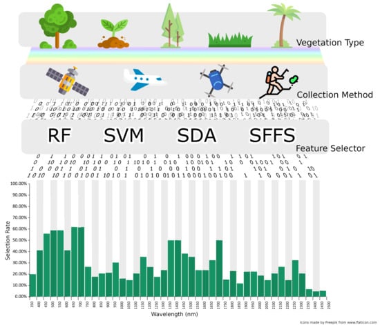
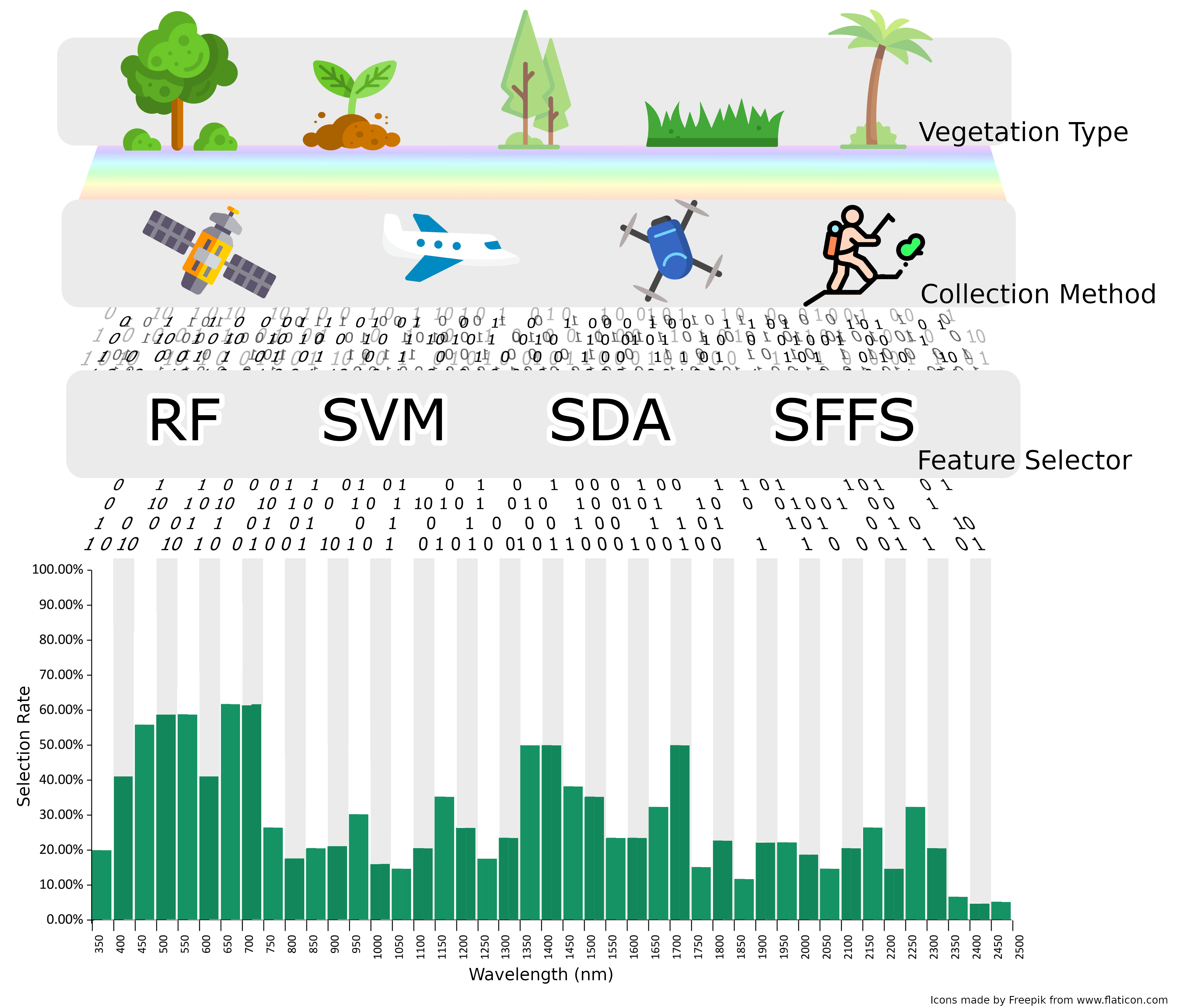
2. Meta-Analysis
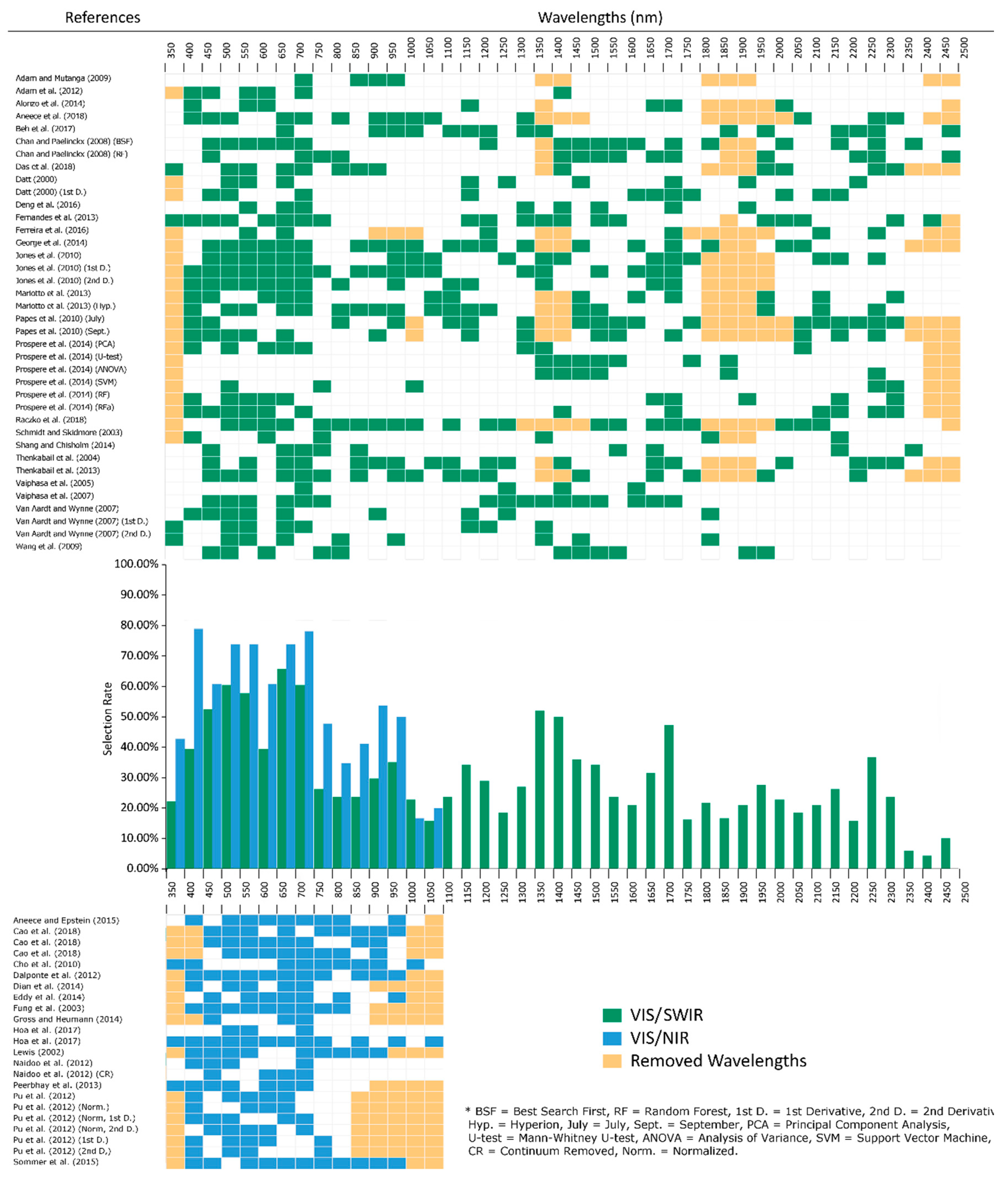
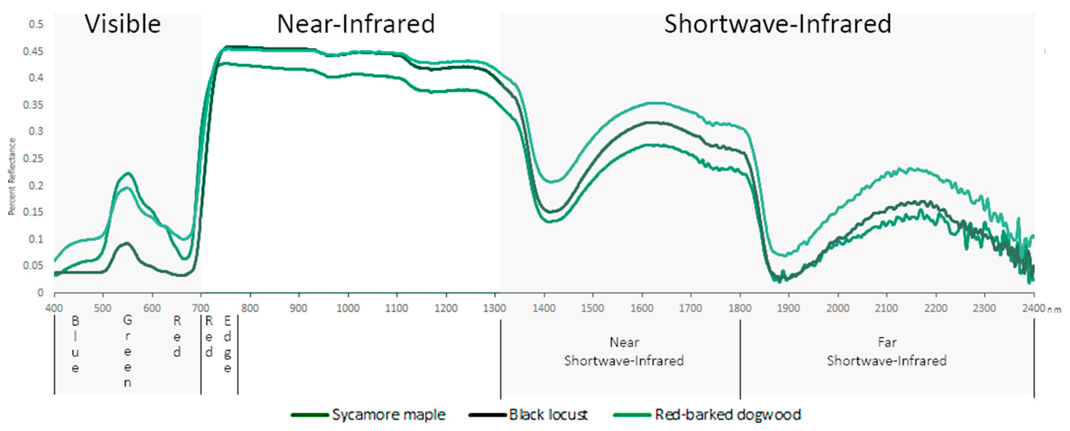
2.1. Spectral Range
2.2. Visible (VIS; 400–700 nm)
2.3. Red Edge (680–780 nm)
2.4. Near Infrared (NIR) (700–1327 nm)
2.5. Shortwave Infrared (SWIR) (1328–2500 nm)
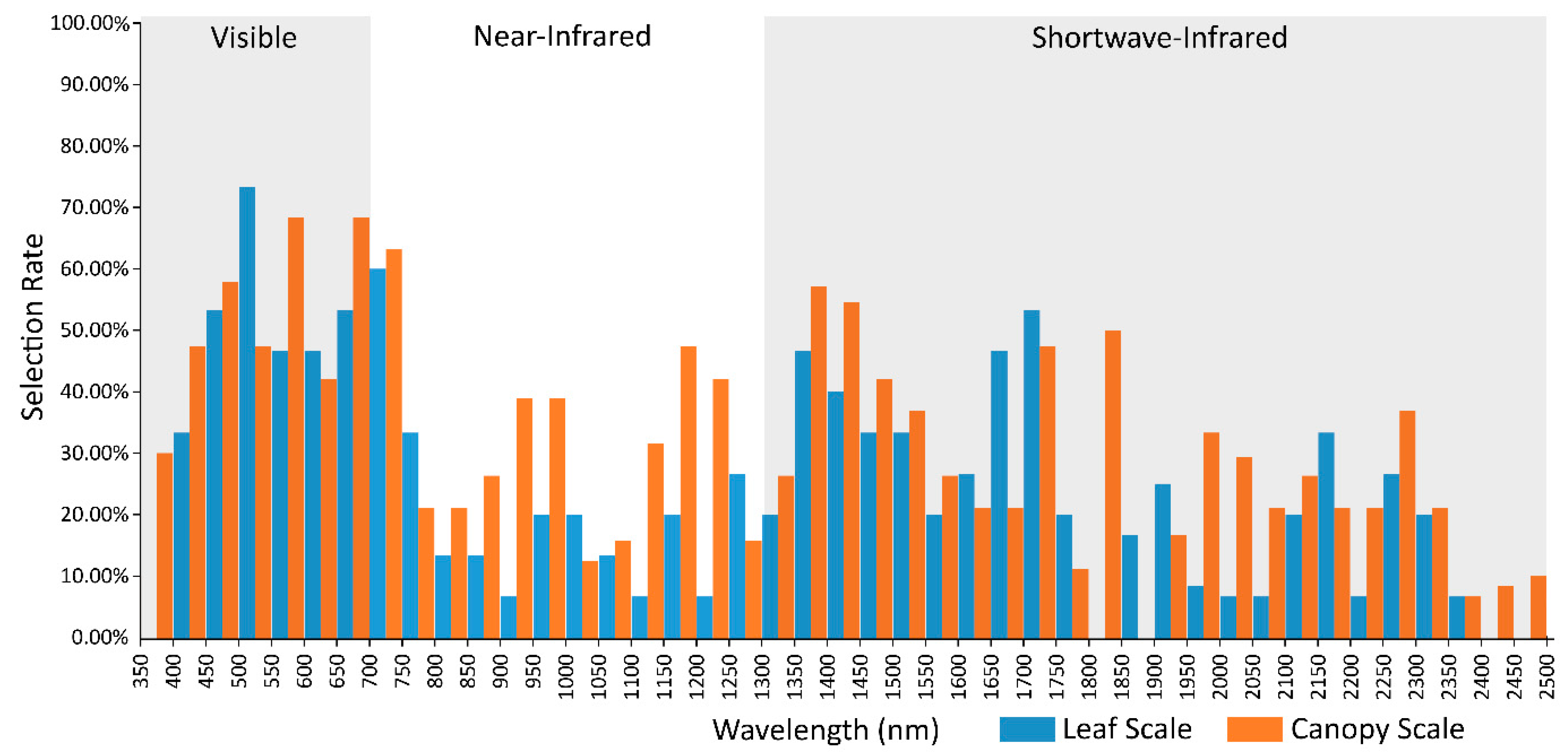
2.6. Canopy and Leaf Scale Spectral Selection Rates
3. Feature Selection
3.1. Filter Methods
3.2. Wrapper Methods
3.3. Embedded Methods
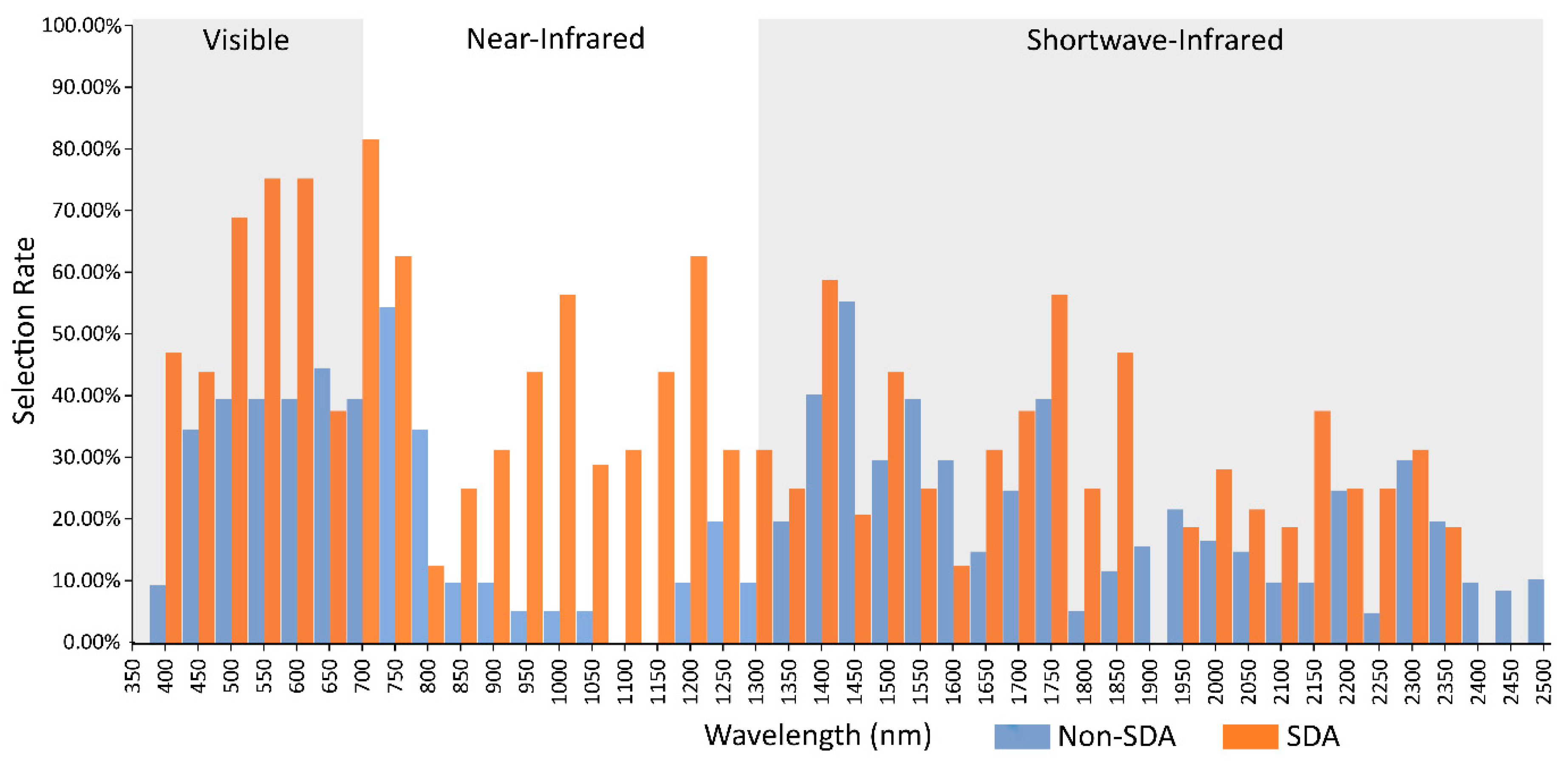
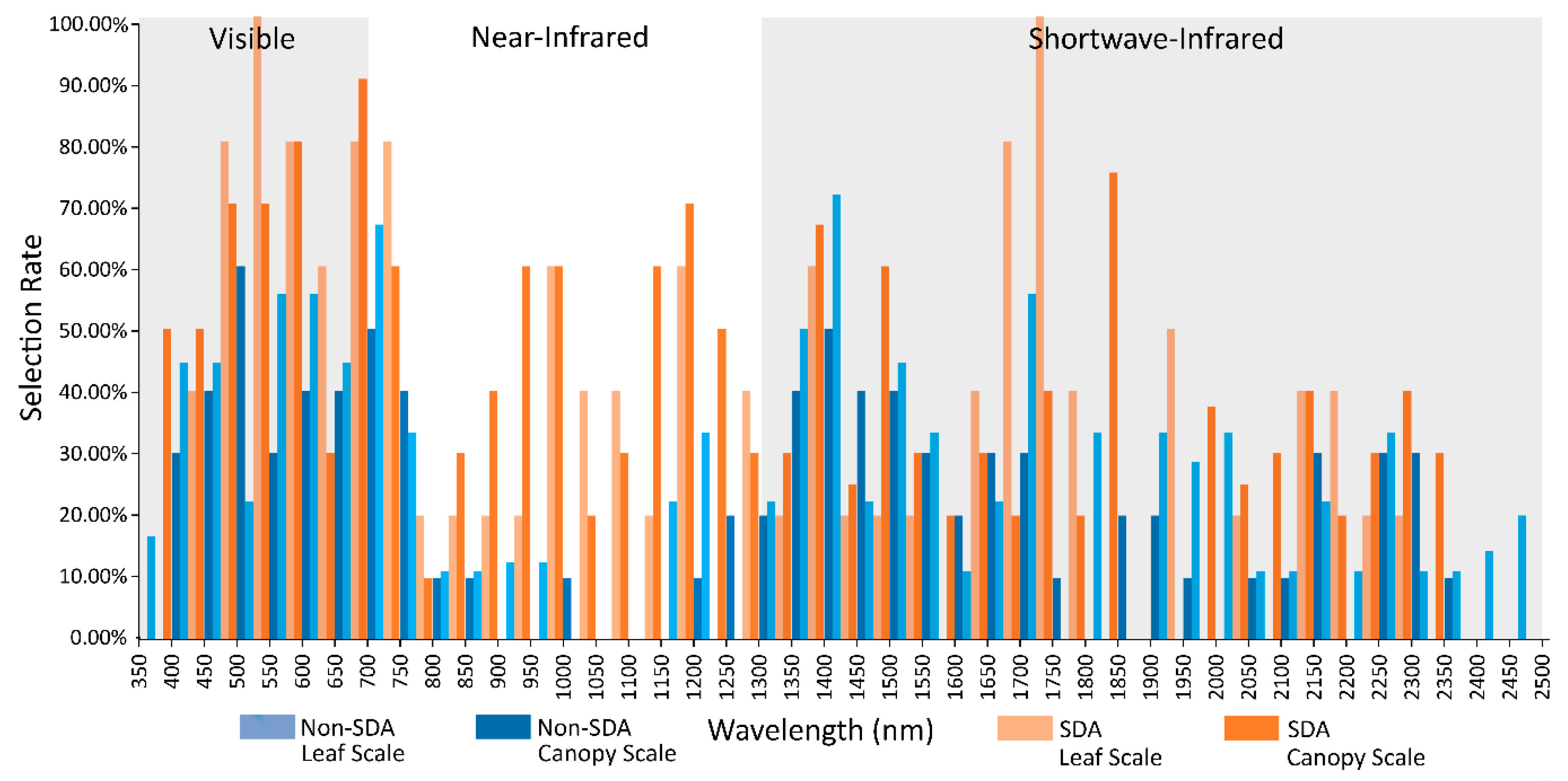
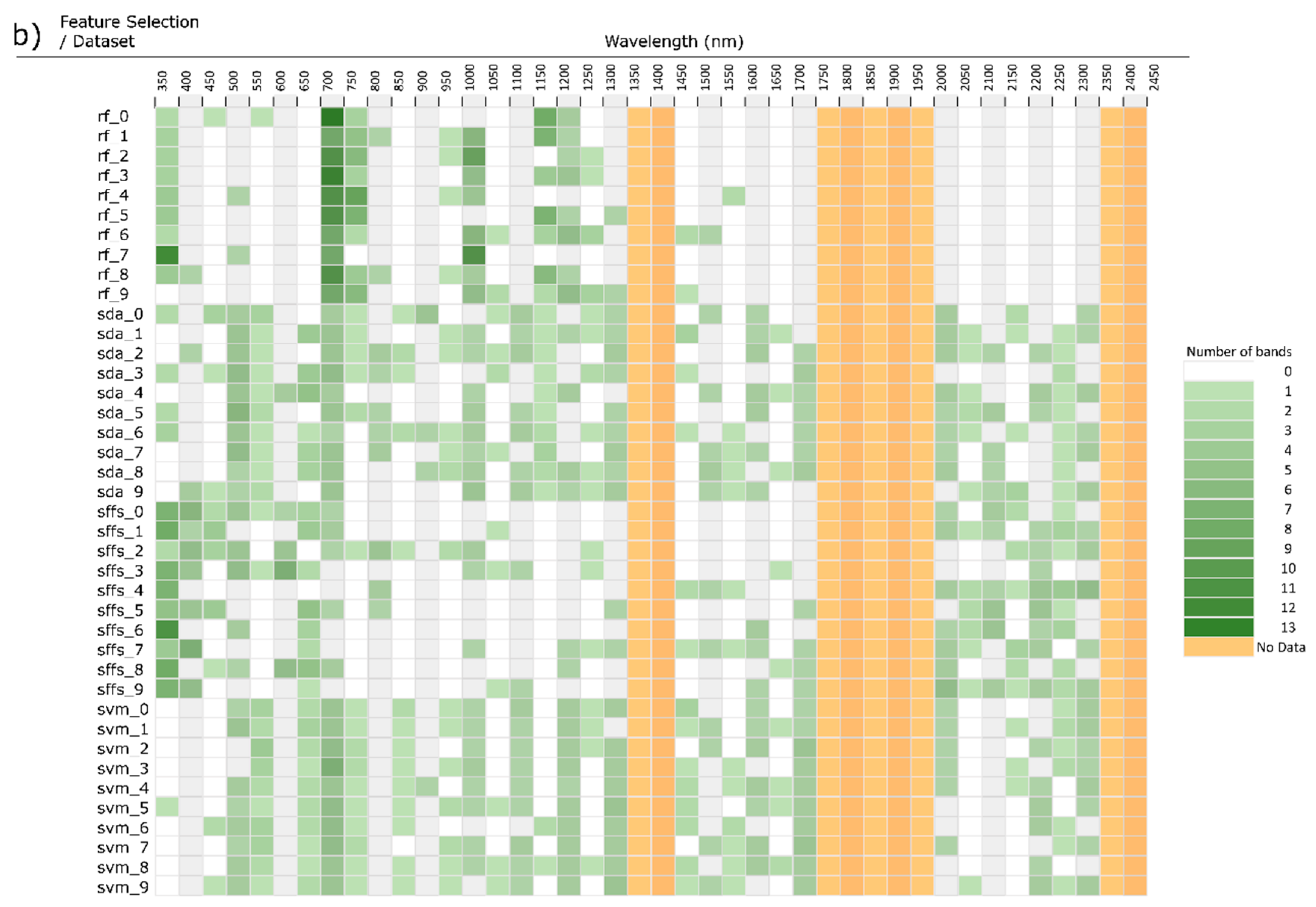
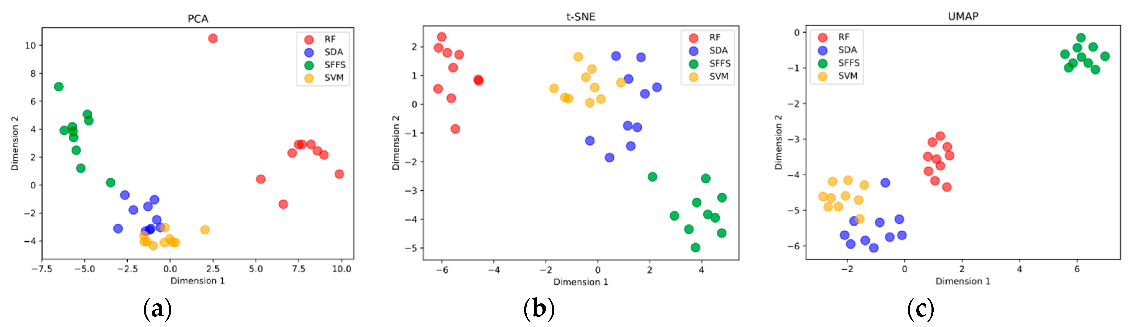
3.4. Comparison of Stepwise Discriminant Analysis (SDA) with non-SDA Feature Selectors
4. Study Design Influence
5. Discussion
6. Conclusions
Author Contributions
Funding
Acknowledgments
Conflicts of Interest
References
- Fassnacht, F.E.; Latifi, H.; Stereńczak, K.; Modzelewska, A.; Lefsky, M.; Waser, L.T.; Straub, C.; Ghosh, A. Review of studies on tree species classification from remotely sensed data. Remote Sens. Environ. 2016, 186, 64–87. [Google Scholar] [CrossRef]
- Fernandes, A.; Melo-Pinto, P.; Millan, B.; Tardaguila, J.; Diago, M. Automatic discrimination of grapevine (Vitis vinifera L.) clones using leaf hyperspectral imaging and partial least squares. J. Agric. Sci. 2015, 153, 455–465. [Google Scholar] [CrossRef]
- Clark, M.L.; Roberts, D.A.; Clark, D.B. Hyperspectral discrimination of tropical rain forest tree species at leaf to crown scales. Remote Sens. Environ. 2005, 96, 375–398. [Google Scholar] [CrossRef]
- Deng, W.; Huang, Y.; Zhao, C.; Chen, L.; Wang, X. Bayesian discriminant analysis of plant leaf hyperspectral reflectance for identification of weeds from cabbages. Afr. J. Agric. Res. 2016, 11, 551–562. [Google Scholar]
- Mariotto, I.; Thenkabail, P.S.; Huete, A.; Slonecker, E.T.; Platonov, A. Hyperspectral versus multispectral crop-productivity modeling and type discrimination for the HyspIRI mission. Remote Sens. Environ. 2013, 139, 291–305. [Google Scholar] [CrossRef]
- Lewis, M. Spectral characterization of Australian arid zone plants. Can. J. Remote Sens. 2002, 28, 219–230. [Google Scholar] [CrossRef]
- Sommer, C.; Holzwarth, S.; Heiden, U.; Heurich, M.; Müller, J.; Mauser, W. Feature based tree species classification using hyperspectral and lidar data in the Bavarian Forest National Park. In Proceedings of the 9th EARSeL Imaging Spectroscopy Workshop, Luxembourg, France, 14–16 April 2015; Volume 14, pp. 49–70. [Google Scholar]
- Prospere, K.; McLaren, K.; Wilson, B. Plant species discrimination in a tropical wetland using in situ hyperspectral data. Remote Sens. 2014, 6, 8494–8523. [Google Scholar] [CrossRef]
- Alonzo, M.; Bookhagen, B.; Roberts, D.A. Urban tree species mapping using hyperspectral and lidar data fusion. Remote Sens. Environ. 2014, 148, 70–83. [Google Scholar] [CrossRef]
- Cho, M.A.; Debba, P.; Mathieu, R.; Naidoo, L.; Van Aardt, J.; Asner, G.P. Improving discrimination of savanna tree species through a multiple-endmember spectral angle mapper approach: Canopy-level analysis. IEEE Trans. Geosci. Remote Sens. 2010, 48, 4133–4142. [Google Scholar] [CrossRef]
- Dalponte, M.; Bruzzone, L.; Gianelle, D. Tree species classification in the Southern Alps based on the fusion of very high geometrical resolution multispectral/hyperspectral images and LiDAR data. Remote Sens. Environ. 2012, 123, 258–270. [Google Scholar] [CrossRef]
- Alonso, M.C.; Malpica, J.A.; de Agirre, A.M. Consequences of the Hughes phenomenon on some classification techniques. In Proceedings of the ASPRS 2011 Annual Conference, Milwaukee, WI, USA, 1–5 May 2011; pp. 1–5. [Google Scholar]
- Hughes, G. On the mean accuracy of statistical pattern recognizers. IEEE Trans. Inf. Theory 1968, 14, 55–63. [Google Scholar] [CrossRef]
- Settles, B. Active Learning Literature Survey; University of Wisconsin-Madison Department of Computer Sciences: Madison, WI, USA, 2009. [Google Scholar]
- Zhu, X.J. Semi-Supervised Learning Literature Survey; University of Wisconsin-Madison Department of Computer Sciences: Madison, WI, USA, 2005. [Google Scholar]
- Van Dyk, D.A.; Meng, X.-L. The art of data augmentation. J. Comput. Graph. Stat. 2001, 10, 1–50. [Google Scholar] [CrossRef]
- Fassnacht, F.E.; Neumann, C.; Förster, M.; Buddenbaum, H.; Ghosh, A.; Clasen, A.; Joshi, P.K.; Koch, B. Comparison of feature reduction algorithms for classifying tree species with hyperspectral data on three central European test sites. IEEE J. Sel. Top. Appl. Earth Obs. Remote Sens. 2014, 7, 2547–2561. [Google Scholar] [CrossRef]
- Richter, R.; Reu, B.; Wirth, C.; Doktor, D.; Vohland, M. The use of airborne hyperspectral data for tree species classification in a species-rich central European forest area. Int. J. Appl. Earth Obs. Geoinf. 2016, 52, 464–474. [Google Scholar] [CrossRef]
- Curran, P.J. Remote sensing of foliar chemistry. Remote Sens. Environ. 1989, 30, 271–278. [Google Scholar] [CrossRef]
- Hennessy, A.; Lewis, M.; Clarke, K. Generative adversarial network synthesis of hyperspectral vegetation data. 2019; Unpublished manuscript, last modified 20 October 2019. [Google Scholar]
- Hueni, A. Field Spectroradiometer Data: Acquisition, Organisation, Processing and Analysis on the Example of New Zealand Native Plants. Master’s Thesis, Massey University, Palmerston North, New Zealand, 2006. [Google Scholar]
- Aneece, I.; Epstein, H. Distinguishing early successional plant communities using ground-level hyperspectral data. Remote Sens. 2015, 7, 16588–16606. [Google Scholar] [CrossRef]
- Cao, J.; Liu, K.; Liu, L.; Zhu, Y.; Li, J.; He, Z. Identifying mangrove species using field close-range snapshot hyperspectral imaging and machine-learning techniques. Remote Sens. 2018, 10, 2047. [Google Scholar] [CrossRef]
- Dian, Y.; Fang, S.; Le, Y.; Xu, Y.; Yao, C. Comparison of the different classifiers in vegetation species discrimination using hyperspectral reflectance data. J. Indian Soc. Remote Sens. 2014, 42, 61–72. [Google Scholar] [CrossRef]
- Eddy, P.; Smith, A.; Hill, B.; Peddle, D.; Coburn, C.; Blackshaw, R. Weed and crop discrimination using hyperspectral image data and reduced bandsets. Can. J. Remote Sens. 2014, 39, 481–490. [Google Scholar] [CrossRef]
- Fung, T.; Yan Ma, H.F.; Siu, W.L. Band selection using hyperspectral data of subtropical tree species. Geocarto Int. 2003, 18, 3–11. [Google Scholar] [CrossRef]
- Gross, J.W.; Heumann, B.W. Can flowers provide better spectral discrimination between herbaceous wetland species than leaves? Remote Sens. Lett. 2014, 5, 892–901. [Google Scholar] [CrossRef]
- Hoa, P.; Giang, N.; Binh, N.; Hieu, N.; Trang, N.; Toan, L.; Long, V.; Ai, T.; Hong, P.; Hai, L. Mangrove species discrimination in southern Vietnam based on in-situ measured hyperspectral reflectance. Int. J. Geoinform. 2017, 13, 25–35. [Google Scholar]
- Naidoo, L.; Cho, M.A.; Mathieu, R.; Asner, G. Classification of savanna tree species, in the greater Kruger national park region, by integrating hyperspectral and LiDAR data in a random forest data mining environment. ISPRS J. Photogramm. Remote Sens. 2012, 69, 167–179. [Google Scholar] [CrossRef]
- Peerbhay, K.Y.; Mutanga, O.; Ismail, R. Commercial tree species discrimination using airborne AISA Eagle hyperspectral imagery and partial least squares discriminant analysis (PLS-DA) in KwaZulu–Natal, South Africa. ISPRS J. Photogramm. Remote Sens. 2013, 79, 19–28. [Google Scholar] [CrossRef]
- Pu, R.; Bell, S.; Baggett, L.; Meyer, C.; Zhao, Y. Discrimination of seagrass species and cover classes with in situ hyperspectral data. J. Coast. Res. 2012, 28, 1330–1344. [Google Scholar] [CrossRef]
- Adam, E.; Mutanga, O. Spectral discrimination of papyrus vegetation (Cyperus papyrus L.) in swamp wetlands using field spectrometry. ISPRS J. Photogramm. Remote Sens. 2009, 64, 612–620. [Google Scholar] [CrossRef]
- Adam, E.; Mutanga, O.; Rugege, D.; Ismail, R. Discriminating the papyrus vegetation (Cyperus papyrus L.) and its co-existent species using random forest and hyperspectral data resampled to HYMAP. Int. J. Remote Sens. 2012, 33, 552–569. [Google Scholar] [CrossRef]
- Aneece, I.; Thenkabail, P. Accuracies achieved in classifying five leading world crop types and their growth stages using optimal earth observing-1 hyperion hyperspectral narrowbands on google earth engine. Remote Sens. 2018, 10, 2027. [Google Scholar] [CrossRef]
- Beh, B.C.; Tan, K.C.; Jafri, M.Z.M.; San Lim, H. Comparison of different discriminant functions for mangrove species analysis in Matang Mangrove Forest Reserve (MMFR), Perak based on statistical approach. In Proceedings of the Remote Sensing for Agriculture, Ecosystems, and Hydrology XIX, Maspalomas, Spain, 14–16 September 2004; p. 104211U. [Google Scholar]
- Chan, J.C.-W.; Paelinckx, D. Evaluation of random forest and adaboost tree-based ensemble classification and spectral band selection for ecotope mapping using airborne hyperspectral imagery. Remote Sens. Environ. 2008, 112, 2999–3011. [Google Scholar] [CrossRef]
- Das, B.; Sahoo, R.N.; Biswas, A.; Pargal, S.; Krishna, G.; Verma, R.; Chinnusamy, V.; Sehgal, V.K.; Gupta, V.K. Discrimination of rice genotypes using field spectroradiometry. Geocarto Int. 2018, 35, 64–77. [Google Scholar] [CrossRef]
- Datt, B. Recognition of eucalyptus forest species using hyperspectral reflectance data. In Proceedings of the IGARSS 2000. IEEE 2000 International Geoscience and Remote Sensing Symposium, Honolulu, HI, USA, 24–28 July 2000; pp. 1405–1407. [Google Scholar]
- Fernandes, M.R.; Aguiar, F.C.; Silva, J.M.; Ferreira, M.T.; Pereira, J.M. Spectral discrimination of giant reed (Arundo donax L.): A seasonal study in riparian areas. ISPRS J. Photogramm. Remote Sens. 2013, 80, 80–90. [Google Scholar] [CrossRef]
- Ferreira, M.P.; Zortea, M.; Zanotta, D.C.; Shimabukuro, Y.E.; de Souza Filho, C.R. Mapping tree species in tropical seasonal semi-deciduous forests with hyperspectral and multispectral data. Remote Sens. Environ. 2016, 179, 66–78. [Google Scholar] [CrossRef]
- George, R.; Padalia, H.; Kushwaha, S. Forest tree species discrimination in western Himalaya using EO-1 Hyperion. Int. J. Appl. Earth Obs. Geoinf. 2014, 28, 140–149. [Google Scholar] [CrossRef]
- Jones, T.G.; Coops, N.C.; Sharma, T. Employing ground-based spectroscopy for tree-species differentiation in the Gulf Islands National Park Reserve. Int. J. Remote Sens. 2010, 31, 1121–1127. [Google Scholar] [CrossRef]
- Papeş, M.; Tupayachi, R.; Martinez, P.; Peterson, A.; Powell, G. Using hyperspectral satellite imagery for regional inventories: A test with tropical emergent trees in the Amazon basin. J. Veg. Sci. 2010, 21, 342–354. [Google Scholar] [CrossRef]
- Raczko, E.; Zagajewski, B. Tree species classification of the UNESCO man and the biosphere karkonoski national park (poland) using artificial neural networks and APEX hyperspectral images. Remote Sens. 2018, 10, 1111. [Google Scholar] [CrossRef]
- Schmidt, K.; Skidmore, A. Spectral discrimination of vegetation types in a coastal wetland. Remote Sens. Environ. 2003, 85, 92–108. [Google Scholar] [CrossRef]
- Shang, X.; Chisholm, L.A. Classification of Australian native forest species using hyperspectral remote sensing and machine-learning classification algorithms. IEEE J. Sel. Top. Appl. Earth Obs. Remote Sens. 2014, 7, 2481–2489. [Google Scholar] [CrossRef]
- Thenkabail, P.S.; Enclona, E.A.; Ashton, M.S.; Van Der Meer, B. Accuracy assessments of hyperspectral waveband performance for vegetation analysis applications. Remote Sens. Environ. 2004, 91, 354–376. [Google Scholar] [CrossRef]
- Thenkabail, P.S.; Mariotto, I.; Gumma, M.K.; Middleton, E.M.; Landis, D.R.; Huemmrich, K.F. Selection of hyperspectral narrowbands (HNBs) and composition of hyperspectral twoband vegetation indices (HVIs) for biophysical characterization and discrimination of crop types using field reflectance and Hyperion/EO-1 data. IEEE J. Sel. Top. Appl. Earth Obs. Remote Sens. 2013, 6, 427–439. [Google Scholar] [CrossRef]
- Vaiphasa, C.; Ongsomwang, S.; Vaiphasa, T.; Skidmore, A.K. Tropical mangrove species discrimination using hyperspectral data: A laboratory study. Estuar. Coast. Shelf Sci. 2005, 65, 371–379. [Google Scholar] [CrossRef]
- Vaiphasa, C.; Skidmore, A.K.; de Boer, W.F.; Vaiphasa, T. A hyperspectral band selector for plant species discrimination. ISPRS J. Photogramm. Remote Sens. 2007, 62, 225–235. [Google Scholar] [CrossRef]
- Van Aardt, J.; Wynne, R. Examining pine spectral separability using hyperspectral data from an airborne sensor: An extension of field-based results. Int. J. Remote Sens. 2007, 28, 431–436. [Google Scholar] [CrossRef]
- Wang, J.; Xu, R.; Yang, S. Estimation of plant water content by spectral absorption features centered at 1450 nm and 1940 nm regions. Environ. Monit. Assess. 2009, 157, 459–469. [Google Scholar] [CrossRef] [PubMed]
- Asner, G.P. Biophysical and biochemical sources of variability in canopy reflectance. Remote Sens. Environ. 1998, 64, 234–253. [Google Scholar] [CrossRef]
- Rivard, B.; Sanchez-Azofeifa, G.; Foley, S.; Calvo-Alvarado, J. Species classification of tropical tree leaf reflectance and dependence on selection of spectral bands. Hyperspect. Remote Sens. Trop. Sub-Trop. For. 2008, 6, 141–159. [Google Scholar]
- Ollinger, S.V. Sources of variability in canopy reflectance and the convergent properties of plants. New Phytol. 2011, 189, 375–394. [Google Scholar] [CrossRef]
- Thenkabail, P.; Smith, R.; De Pauw, E. Hyperspectral Vegetation Indices for Determining Agricultural Crop Characteristics, CEO Research Publication Series No. 1; Center for Earth Observation, Yale University Press: New Haven, CT, USA, 1999. [Google Scholar]
- Thenkabail, P.S.; Smith, R.B.; De Pauw, E. Evaluation of narrowband and broadband vegetation indices for determining optimal hyperspectral wavebands for agricultural crop characterization. Photogramm. Eng. Remote Sens. 2002, 68, 607–622. [Google Scholar]
- Ferreira, M.P.; Grondona, A.E.B.; Rolim, S.B.A.; Shimabukuro, Y.E. Analyzing the spectral variability of tropical tree species using hyperspectral feature selection and leaf optical modeling. J. Appl. Remote Sens. 2013, 7, 073502. [Google Scholar] [CrossRef]
- Galvão, L.S.; Roberts, D.A.; Formaggio, A.R.; Numata, I.; Breunig, F.M. View angle effects on the discrimination of soybean varieties and on the relationships between vegetation indices and yield using off-nadir Hyperion data. Remote Sens. Environ. 2009, 113, 846–856. [Google Scholar] [CrossRef]
- Blackburn, G.A. Hyperspectral remote sensing of plant pigments. J. Exp. Bot. 2006, 58, 855–867. [Google Scholar] [CrossRef] [PubMed]
- Thomas, J.; Gausman, H. Leaf reflectance vs. leaf chlorophyll and carotenoid concentrations for eight crops. Agron. J. 1977, 69, 799–802. [Google Scholar] [CrossRef]
- Castro-Esau, K.L.; Sánchez-Azofeifa, G.A.; Rivard, B.; Wright, S.J.; Quesada, M. Variability in leaf optical properties of Mesoamerican trees and the potential for species classification. Am. J. Bot. 2006, 93, 517–530. [Google Scholar] [CrossRef]
- Pu, R. Broadleaf species recognition with in situ hyperspectral data. Int. J. Remote Sens. 2009, 30, 2759–2779. [Google Scholar] [CrossRef]
- Demmig-Adams, B.; Adams, W.W. The role of xanthophyll cycle carotenoids in the protection of photosynthesis. Trends Plant Sci. 1996, 1, 21–26. [Google Scholar] [CrossRef]
- Gamon, J.; Penuelas, J.; Field, C. A narrow-waveband spectral index that tracks diurnal changes in photosynthetic efficiency. Remote Sens. Environ. 1992, 41, 35–44. [Google Scholar] [CrossRef]
- Gitelson, A.A.; Merzlyak, M.N.; Chivkunova, O.B. Optical properties and nondestructive estimation of anthocyanin content in plant leaves. Photochem. Photobiol. 2001, 74, 38–45. [Google Scholar] [CrossRef]
- Gong, P.; Pu, R.; Yu, B. Conifer species recognition: An exploratory analysis of in situ hyperspectral data. Remote Sens. Environ. 1997, 62, 189–200. [Google Scholar] [CrossRef]
- Van Aardt, J.A. Spectral separability among six southern tree species. Photogramm. Eng. Remote Sens. 2001, 67, 1367–1375. [Google Scholar]
- Karlovska, A.; Grīnfelde, I.; Alsiņa, I.; Priedītis, G.; Roze, D. Plant reflected spectra depending on biological characteristics and growth conditions. In Proceedings of the International Scientific Conference Rural Development, Akademija, Lithuania, 23–24 November 2017. [Google Scholar]
- Clevers, J.; De Jong, S.; Epema, G.; Van Der Meer, F.; Bakker, W.; Skidmore, A.; Scholte, K. Derivation of the red edge index using the MERIS standard band setting. Int. J. Remote Sens. 2002, 23, 3169–3184. [Google Scholar] [CrossRef]
- Dawson, T.; Curran, P. Technical note A new technique for interpolating the reflectance red edge position. Int. J. Remote Sens. 1998, 19, 2133–2139. [Google Scholar] [CrossRef]
- Gholizadeh, A.; Mišurec, J.; Kopačková, V.; Mielke, C.; Rogass, C. Assessment of red-edge position extraction techniques: A Case study for norway spruce forests using hymap and simulated sentinel-2 data. Forests 2016, 7, 226. [Google Scholar] [CrossRef]
- Dalponte, M.; Bruzzone, L.; Vescovo, L.; Gianelle, D. The role of spectral resolution and classifier complexity in the analysis of hyperspectral images of forest areas. Remote Sens. Environ. 2009, 113, 2345–2355. [Google Scholar] [CrossRef]
- Cochrane, M. Using vegetation reflectance variability for species level classification of hyperspectral data. Int. J. Remote Sens. 2000, 21, 2075–2087. [Google Scholar] [CrossRef]
- Rock, B.; Hoshizaki, T.; Miller, J. Comparison of in situ and airborne spectral measurements of the blue shift associated with forest decline. Remote Sens. Environ. 1988, 24, 109–127. [Google Scholar] [CrossRef]
- Knipling, E.B. Physical and physiological basis for the reflectance of visible and near-infrared radiation from vegetation. Remote Sens. Environ. 1970, 1, 155–159. [Google Scholar] [CrossRef]
- Kumar, L. A comparison of reflectance characteristics of some Australian eucalyptus species based on high spectral resolution data—Discriminating using the visible and NIR regions. J. Spat. Sci. 2007, 52, 51–64. [Google Scholar] [CrossRef]
- Kumar, L.; Skidmore, A.K.; Mutanga, O. Leaf level experiments to discriminate between eucalyptus species using high spectral resolution reflectance data: Use of derivatives, ratios and vegetation indices. Geocarto Int. 2010, 25, 327–344. [Google Scholar] [CrossRef]
- Elvidge, C.D. Visible and near infrared reflectance characteristics of dry plant materials. Remote Sens. 1990, 11, 1775–1795. [Google Scholar] [CrossRef]
- Lehmann, J.R.K.; Große-Stoltenberg, A.; Römer, M.; Oldeland, J. Field spectroscopy in the VNIR-SWIR region to discriminate between Mediterranean native plants and exotic-invasive shrubs based on leaf tannin content. Remote Sens. 2015, 7, 1225–1241. [Google Scholar] [CrossRef]
- Kokaly, R.F.; Asner, G.P.; Ollinger, S.V.; Martin, M.E.; Wessman, C.A. Characterizing canopy biochemistry from imaging spectroscopy and its application to ecosystem studies. Remote Sens. Environ. 2009, 113, S78–S91. [Google Scholar] [CrossRef]
- Alonso-Atienza, F.; Rojo-Álvarez, J.L.; Rosado-Muñoz, A.; Vinagre, J.J.; García-Alberola, A.; Camps-Valls, G. Feature selection using support vector machines and bootstrap methods for ventricular fibrillation detection. Expert Syst. Appl. 2012, 39, 1956–1967. [Google Scholar] [CrossRef]
- Pudil, P.; Novovičová, J.; Kittler, J. Floating search methods in feature selection. Pattern Recognit. Lett. 1994, 15, 1119–1125. [Google Scholar] [CrossRef]
- Guyon, I.; Weston, J.; Barnhill, S.; Vapnik, V. Gene selection for cancer classification using support vector machines. Mach. Learn. 2002, 46, 389–422. [Google Scholar] [CrossRef]
- Deng, H.; Runger, G. Feature selection via regularized trees. In Proceedings of the 2012 International Joint Conference on Neural Networks (IJCNN), Dallas, TX, USA, 4–9 August 2013; pp. 1–8. [Google Scholar]
- Melgani, F.; Bruzzone, L. Classification of hyperspectral remote sensing images with support vector machines. IEEE Trans. Geosci. Remote Sens. 2004, 42, 1778–1790. [Google Scholar] [CrossRef]
- Pal, M.; Mather, P.M. Assessment of the effectiveness of support vector machines for hyperspectral data. Future Gener. Comput. Syst. 2004, 20, 1215–1225. [Google Scholar] [CrossRef]
- Pal, M.; Foody, G.M. Feature selection for classification of hyperspectral data by SVM. IEEE Trans. Geosci. Remote Sens. 2010, 48, 2297–2307. [Google Scholar] [CrossRef]
- Breiman, L. Random forests. Mach. Learn. 2001, 45, 5–32. [Google Scholar] [CrossRef]
- Huberty, C.J. Applied Discriminant Analysis; Wiley-Interscience: New York, NY, USA, 1994. [Google Scholar]
- Thompson, B. Why Wont Stepwise Methods Die; American Counseling Association: Alexandria, VA, USA, 1989. [Google Scholar]
- Thompson, B. Stepwise Regression and Stepwise Discriminant Analysis Need Not Apply Here: A Guidelines Editorial; SAGE Publications: Thousand Oaks, CA, USA, 1995. [Google Scholar]
- Flom, P.L.; Cassell, D.L. Stopping stepwise: Why stepwise and similar selection methods are bad, and what you should use. In Proceedings of the NorthEast SAS Users Group Inc 20th Annual Conference, Baltimore, MD, USA, 11–14 November 2007. [Google Scholar]
- Whitaker, J.S. Use of Stepwise Methodology in Discriminant Analysis; The Annual Meeting of the Southwest Educational Research Association; Texas A & M University: College Station, TX, USA, 1997; p. 18. [Google Scholar]
- Huberty, C.J.; Barton, R.M. An Introduction to Discriminant Analysis. Meas. Eval. Couns. Dev. 1989, 22, 158–168. [Google Scholar] [CrossRef]


| References | Wavelengths/Bandwidths | Classes | Pre-Processing | Feature Selection Method | No. Bands Selected | Accuracy % | Study Context and Spatial Scale or Resolution |
|---|---|---|---|---|---|---|---|
| [22] | 350–1025 nm, 3 nm | 12 | Band depth | Segmented PCA | 12 | 77.0 | Successional plant communities from canopy field spectra |
| [23] | 454–950 nm, 4 nm | 8 | Smoothing | SDA | 14 | 91.4 | Mangrove forest field canopy spectra |
| [23] | 454–950 nm, 4 nm | 8 | Smoothing | CFS | 23 | 92.3 | Mangrove forest field canopy spectra |
| [23] | 454–950 nm, 4 nm | 8 | Smoothing | SPA | 23 | 93.1 | Mangrove forest field canopy spectra |
| [10] | 384.8–1054.3 nm, 9.23 nm | 10 | SAM Band Selector Addon | 31 | 53.0 | Savanna tree species from airborne imagery (1.12 m) | |
| [11] | 403–989 nm, 4.6 nm | 8 | Sequential Forward Floating Selection | 43 | 74.1 | Alpine tree species and 2 non-species classes, airborne imagery (1 m) | |
| [24] | 400–900 nm, 1 nm | 13 | Spec angle and dist., feature parameters | 7 | 96.2 | Varied plant species from lab leaf spectra | |
| [25] | 400–1000 nm, 10 nm | 5 | PCA, SDA, Manual selection | 7 | ~91.4 | Crop and weed species from field imagery (1.25 m) | |
| [26] | 400–900 nm, 2.6 nm | 25 | Smoothing | Hierarchical Clustering | 13 | 89.0 | Sub-tropical tree species from lab leaf spectra |
| [27] | 475–900 nm, 1 nm | 22 | Forward Feature Selection | 8 | 43.0 | Herbaceous wetland species from field leaf spectra | |
| [28] | 325–1075 nm, 2 nm | 6 | Smoothing | SDA | 6 | 92.0 | Mangrove forest field canopy spectra |
| [28] | 325–1075 nm, 2 nm | 6 | Smoothing, CR | SDA | 17 | 93.6 | Mangrove forest field canopy spectra |
| [6] | 400–900 nm, 1.4 nm | 8 | PCA, Discriminant Analysis | 13 | 57.0 | Arid zone plant groups from field leaf spectra | |
| [29] | 384.8–1054.3, 9.23 nm | 9 | Random Forest, Gini Index | 8 | 80.3 | Savanna tree species from airborne imagery (1.3 m) | |
| [29] | 384.8–1054.3, 9.23 nm | 9 | Continuum removed | Random Forest, Gini Index | 9 | ~79.0 | Savanna tree species from airborne imagery (1.3 m) |
| [30] | 393–900 nm, 2.2 nm | 6 | PLSDA VIP score | 78 | 88.8 | Forestry species from airborne imagery (2.4 m) | |
| [31] | 400–800 nm, 3 nm | 3 | Two Sample T-test | 5 | 69.1 | Seagrass species field canopy spectra | |
| [31] | 400–800 nm, 3 nm | 3 | Normalized | Two Sample T-test | 5 | 66.0 | Seagrass species field canopy spectra |
| [31] | 400–800 nm, 3 nm | 3 | Normalized 1st Derivative | Two Sample T-test | 5 | 71.1 | Seagrass species field canopy spectra |
| [31] | 400–800 nm, 3 nm | 3 | Normalized 2nd Derivative | Two Sample T-test | 5 | 73.2 | Seagrass species field canopy spectra |
| [31] | 400–800 nm, 3 nm | 3 | 1st Derivative | Two Sample T-test | 5 | 69.1 | Seagrass species field canopy spectra |
| [31] | 400–800 nm, 3 nm | 3 | 2nd Derivative | Two Sample T-test | 5 | 67.0 | Seagrass species field canopy spectra |
| [7] | 400–1000 nm, 3 nm | 13 | Normalisation | PCA, Correlation matrix, Band variance | 53 | 77.0 | European forest trees species from airborne imagery (1.6 m) |
| References | Wavelengths/Bandwidths | Classes | Pre-processing | Feature Selection Method | Bands | Accuracy % | Study Context and Spatial Scale or Resolution |
|---|---|---|---|---|---|---|---|
| [32] | 350–2500 nm @ 3, 10 nm | 4 | ANOVA, CART | 8 | 97.4 | Wetland species from field canopy spectra | |
| [33] | 350–2500 nm @ 3, 10 nm | 4 | Resampled | Random Forest | 10 | 90.5 | Wetland species from field canopy spectra |
| [9] | 385–2450 nm @ 9.6 nm | 29 | Forward Feature Selection | 7 | 79.2 | Urban street tree species from airborne imagery (3.7 m) | |
| [34] | 427–2355 nm @ 10 nm | 4 | PCA | 15 | 86.3 | Agricultural crops, Hyperion (30 m) | |
| [35] | 350–2500 nm @ 10nm | 6 | Resampled | ANOVA, LDA | 26 | 77.0 | Mangrove species leaf scale |
| [36] | 400–2500 nm @ 16 nm | 16 | Best-First Search Algorithm | 21 | ~69.5 | Temperate forest ecotopes from airborne imagery (4 m) | |
| [36] | 400–2500 nm @ 16 nm | 16 | Random Forest | 21 | ~69.5 | Temperate forest ecotopes from airborne imagery (4 m) | |
| [37] | 350–2350 nm @ 1 nm | 14 | ANOVA (Tukey HSD), CART | 17 | 98.0 | Rice genotypes from canopy spectra | |
| [38] | 400–2500 nm @ 10 nm | 7 | Resampled | SDA | 12 | 70.4 | Eucalypt forest species from lab leaf spectra |
| [38] | 400–2500 nm @ 10 nm | 7 | Resampled, 1st Derivative | SDA | 13 | 72.4 | Eucalypt forest species from lab leaf spectra |
| [4] | 350–2500 nm @ 1.4, 2 nm | 7 | PCA | 8 | 84.3 | Cabbage crops and weed species from field canopy spectra | |
| [39] | 350–2450 nm @ 3, 10nm | 4 | Kruskal-Wallis post hoc Dunn, CART | 56 | ~95 | Giant Reed and coexisting vegetation from field canopy spectra | |
| [40] | 400–2400 nm @ 4, 6 nm | 8 | Smoothing | Stepwise Regression Wrapper | 30 | ~70.0 | Tropical tree species from airborne imagery (1 m) |
| [41] | 400–2350 nm @ 10 nm | 6 | Continuum Removed | SDA | 29 | 82.3 | Himalayan forest species from satellite imagery (30 m) |
| [42] | 429–2400 nm @ 2 nm | 11 | SDA | 40 | ~98.0 | Canadian forest tree species from lab leaf spectra | |
| [42] | 429–2400 nm @ 2 nm | 11 | 1st Derivative | SDA | 40 | ~98.0 | Canadian forest tree species from lab leaf spectra |
| [42] | 429–2400 nm @ 2 nm | 11 | 2nd Derivative | SDA | 40 | ~98.0 | Canadian forest tree species from lab leaf spectra |
| [5] | 426.5–2355 nm @ 10 nm | 5 | LS-means, SDA, PCA, LL-R2 | 29 | 90.2 | Crop species from satellite imagery (30 m) | |
| [5] | 426.5–2355 nm @ 10 nm | 5 | Resampled | LS-means, SDA, PCA, LL-R2 | 21 | 92.0 | Crop species from canopy field spectra |
| [43] | 415–2340 nm @ 10 nm | 5 | SDA | 25 | 100 | Amazon tree species from satellite imagery (30 m) | |
| [43] | 415–2340 nm @ 10 nm | 5 | SDA | 25 | 100 | Amazon tree species from satellite imagery (30 m) | |
| [8] | 400–2400 nm @ 5 nm | 46 | Smoothing, Normalization | PCA | 20 | 82.6 | Tropical wetland species from field leaf spectra |
| [8] | 400–2400 nm @ 5 nm | 46 | Smoothing, Normalization | Mann-Whitney U-test | 21 | 86.8 | Tropical wetland species from field leaf spectra |
| [8] | 400–2400 nm @ 5 nm | 46 | Smoothing, Normalization | ANOVA | 23 | 83.4 | Tropical wetland species from field leaf spectra |
| [8] | 400–2400 nm @ 5 nm | 46 | Smoothing, Normalization | SVM | 20 | 87.1 | Tropical wetland species from field leaf spectra |
| [8] | 400–2400 nm @ 5 nm | 46 | Smoothing, Normalization | Random Forest | 20 | 86.1 | Tropical wetland species from field leaf spectra |
| [8] | 400–2400 nm @ 5 nm | 46 | Smoothing, Normalization | Random Forest (a) | 20 | 84.8 | Tropical wetland species from field leaf spectra |
| [44] | 413–2440 nm @ 0.6, 11 nm | 6 | PCA | 40 | 87.0 | ||
| [45] | 400–2500 nm @ 2, 6, 10 nm | 27 | Smoothing, Continuum removed | Mann-Whitney U-test, Manual Selection | 6 | - | Saltmarsh vegetation types from field canopy spectra |
| [46] | 350–2500 nm @ 3, 10 nm | 7 | ANOVA – post hoc Tukey-Kramer | 9 | 94.7 | Australian forest species from lab leaf spectra | |
| [47] | 390–2360 nm @ 10 nm | 4 | Resampled | PCA, LL-R2, SDA, DGVI | 22 | 97.0 | Crops and savanna cover types from field canopy spectra |
| [48] | 350–2350 nm @ 10 nm | 8 | SDA | 20 | 95.0 | Crop types from field canopy spectra | |
| [49] | 350–2500 nm @ 3, 10 nm | 16 | Genetic Algorithm | 4 | ~80.0 | Mangrove species from lab leaf spectra | |
| [50] | 350–2500 nm @ 3, 10 nm | 16 | Genetic Algorithm | (30*4) | ~80.0 | Mangrove species from lab leaf spectra | |
| [51] | 400–2500 nm @ 10 nm | 3 | SDA | 10 | 65.0 | Pine tree species from airborne imagery (3.4 m) | |
| [51] | 400–2500 nm @ 10 nm | 3 | 1st Derivative | SDA | 10 | 77.0 | Pine tree species from airborne imagery (3.4 m) |
| [51] | 400–2500 nm @ 10 nm | 3 | 2nd Derivative | SDA | 10 | 72. | Pine tree species from airborne imagery (3.4 m) |
| [52] | 350–2500 nm @ 10 nm | 3 | Resampled | ANOVA, LDA | 15 | 90.0 | Mangrove species from lab leaf spectra |
| Feature Selector | Software Package and Library | Hyperpaprametes |
|---|---|---|
| SVM | Python 3.6, scikit-learn v0.21.3 | C = 100, class_weight = ‘balanced’, kernel = ‘linear’ |
| SDA | Python 3.6, milk v0.6.1 | tolerance = 0.001, significance_in = 0.01, significance_out = 0.01, Metric = ‘Wilk’s Lambda’ |
| SFFS | R 3.6.1, varSel v0.1 | Metric = “Jeffries-Matusita distance”, Strategy = "mean" |
| RF | Python 3.6, scikit-learn v0.21.3 | n_estimators = 100, criterion = ‘gini’, max_depth = None, min_samples_leaf = 1 |
© 2020 by the authors. Licensee MDPI, Basel, Switzerland. This article is an open access article distributed under the terms and conditions of the Creative Commons Attribution (CC BY) license (http://creativecommons.org/licenses/by/4.0/).
Share and Cite
Hennessy, A.; Clarke, K.; Lewis, M. Hyperspectral Classification of Plants: A Review of Waveband Selection Generalisability. Remote Sens. 2020, 12, 113. https://doi.org/10.3390/rs12010113
Hennessy A, Clarke K, Lewis M. Hyperspectral Classification of Plants: A Review of Waveband Selection Generalisability. Remote Sensing. 2020; 12(1):113. https://doi.org/10.3390/rs12010113
Chicago/Turabian StyleHennessy, Andrew, Kenneth Clarke, and Megan Lewis. 2020. "Hyperspectral Classification of Plants: A Review of Waveband Selection Generalisability" Remote Sensing 12, no. 1: 113. https://doi.org/10.3390/rs12010113
APA StyleHennessy, A., Clarke, K., & Lewis, M. (2020). Hyperspectral Classification of Plants: A Review of Waveband Selection Generalisability. Remote Sensing, 12(1), 113. https://doi.org/10.3390/rs12010113