Modeling Hyperspectral Response of Water-Stress Induced Lettuce Plants Using Artificial Neural Networks

Abstract

Modeling the hyperspectral response of vegetables is important for estimating water stress through a noninvasive approach. This article evaluates the hyperspectral response of water-stress induced lettuce (Lactuca sativa L.) using artificial neural networks (ANN). We evenly split 36 lettuce pots into three groups: control, stress, and bacteria. Hyperspectral response was measured four times, during 14 days of stress induction, with an ASD Fieldspec HandHeld spectroradiometer (325–1075 nm). Both reflectance and absorbance measurements were calculated. Different biophysical parameters were also evaluated. The performance of the ANN approach was compared against other machine learning algorithms. Our results show that the ANN approach could separate the water-stressed lettuce from the non-stressed group with up to 80% accuracy at the beginning of the experiment. Additionally, this accuracy improved at the end of the experiment, reaching an accuracy of up to 93%. Absorbance data offered better accuracy than reflectance data to model it. This study demonstrated that it is possible to detect early stages of water stress in lettuce plants with high accuracy based on an ANN approach applied to hyperspectral data. The methodology has the potential to be applied to other species and cultivars in agricultural fields.

1. Introduction

Remote sensing is an important tool for the analysis of vegetation in agricultural fields because it allows farmers to obtain data in a faster manner than most traditional methods [1,2]. Changes in the spectral response of plants can be observed with equipment that records wavelength values, such as a spectroradiometer [3]. The analysis of the spectral signatures enables the identification of vegetation characteristics that would not be visually perceived in asymptomatic plants [4]. Because of this, many studies focusing on phytosanitary problems are based on spectroscopy. These problems include nutritional deficiencies [5,6,7]; diseases [8], biomass [9], and, as in the present study, water stress [10].

The spectral response of a plant differs according to the species, which motivates the creation of different approaches to model it [11]. One of the problems commonly faced by farmers is related to water stress, which limits growth and compromises its production [12]. Water stress is responsible for chlorophyll variation and impairing other biological components, such as leaf area and root size [13]. The alteration of these components results in the appearance of visual symptoms, but they are difficult to identify due to their similarity to other problems, such as diseases, malnutrition, and cold damage [14]. An alternative that can identify changes caused by water stress alone is hyperspectral analysis [10,11].

The amount of leaf water is best estimated in the near-infrared and medium-infrared spectral regions [15]. In the near-infrared region, the spectral response is associated with the structural organization of intracellular molecules located in the mesophyll, which is affected as a consequence of stress [14]. Stress may also unbalance other physiological conditions and cause changes in visible and red-edge regions [15]. Changes in these spectral regions are associated with foliar pigmentation. Studies have sought to evaluate spectral behavior in these and other regions of the spectrum [16,17]. In addition, the absorbance curve has shown a better relationship with leaf pigmentation [18], which encourages the use of absorbance data to evaluate the negative effects caused by stress in plants.

Different approaches have been adopted to model the hyperspectral response when detecting water stress in cultures. In rice, multivariate analysis models were applied to determine the spectral response of the plant under different stress levels [10]. In tomatoes, classification trees were used to separate the spectral indices that best corresponded to the induced water stress [12]. In winter wheat crops, through continuous analysis of hyperspectral data over time, it was possible to quantify water stress in relation to other variables, such as disease and nitrogen accumulation [19]. Other studies have evaluated the implications of water stress through hyperspectral data in different plants, such as vineyards [11] and citrus fruits [20].

Recently, machine learning approaches have been used in modeling the hyperspectral response of different conditions associated with vegetation [21]. The popular techniques used for analyzing data include regression analysis, vegetation indices, linear polarizations, wavelet-based filtering, and, currently, machine learning algorithms like random forest, decision tree, support vector machine (SVM), k-nearest neighbor (kNN), artificial neural networks (ANN), naïve Bayes (NB), and others [22,23,24,25]. To evaluate the hyperspectral response of plants, machine learning has already been implemented in different scenarios. A radial basis function and the kNN were used to detect citrus canker in several disease development stages [26]. ANN, NB, and kNN were also used to model pepper fusarium disease in a climate room [27]. A combination of different machine learning algorithms like SVM, ANN, and others were also evaluated to model photosynthetic variables [28].

In lettuce, water stress poses a major threat. To deal with this, commercially available seeds are being inoculated with rhizobacteria, because it mitigates the effects of the stress [29]. These effects; however, may not be visually perceptible, which makes detection by ordinary approaches difficult. Hyperspectral data have already demonstrated high potential in assessing water stress in plants in different spectral regions (350–2500 nm) [11,23,30]. However, to date, no model has evaluated the spectral response of lettuce submitted to water stress. Here we evaluate the hyperspectral response of water-stress induced lettuce with a machine learning method through ANN. The contribution of this study is twofold. Firstly, we identified the effects of water stress in lettuce and its association with their spectral response. Secondly, we evaluated the performance of the ANN algorithm to model its effects. The rest of this article is organized as follows. Section 2 presents the materials and methods adopted in this study. Section 3 and Section 4 present and discuss the results obtained in the experimental analysis. Finally, Section 5 concludes the article.

2. Materials and Methods

The experiment was conducted in a growth chamber under controlled conditions in a phytotron. Twenty-eight-day-old lettuce (Lactuca sativa L.) plants were transplanted to pots with 0.5 kg of agricultural soil (pH (CaCl₂ 0.01 mol L⁻¹) 5.9; 43.9 mg dm-3 of P (Mehlich-1), 2.7 mmol dm-3 of K, 25.3 mmol dm-3 of Ca, 5.3 mmol dm-3 of Mg, 14.3 mmol dm-3 of H + Al). The experimental design was randomized with three treatments (n = 36). One treatment was carried out with B. subtilis inoculation, strain AP-3 [31]. The inoculation was performed with bacteria obtained by scraping cells multiplied in a solid medium, diluted in sterile water to a concentration of 1.0.109 cels. mL⁻¹, and 0.1 mL per inoculum. The plants were cultivated for 14 days under the same irrigation conditions, maintaining the soil at field capacity. From the 14th day on, water restriction was applied.

The treatments were conducted as follows: (i) control group, with maintenance of the field capacity and without inoculation of the plants; (ii) stress group, with maintenance of 50% of the field capacity and without inoculation of the plants, and; (iii) bacteria group, with maintenance of 50% of field capacity and inoculation of the plants. The water replacement for field capacity maintenance of only 50% was conducted by the gravimetric method. The phytotron chamber maintained the same temperature (25 °C) and lighting conditions during the experiment. Water-deficit treatment was performed for 15 days and was completed on the 30th day after the transplantation of the plants to vessels. The experimental design and analysis are summarized below (Figure 1).

2.1. Spectral Data Measurements

To record the spectral response of each plant, considering the different treatments, a darkroom was prepared to avoid light interference from other materials. The spectral response of the lettuce was measured using a Fieldspec HandHeld ASD spectroradiometer, operating at a spectral range of 325–1075 nm, in 512 channels with a spectral resolution of 1.6 nm and a 1° field of view. The equipment was carefully placed close to the leaves, at a 45° inclination, in relation to the height of the plant so that its field of view (FOV) did not exceed the area of the plant and register the spectral response of the substrate. A halogenic lamp was also placed at 45° on the other side. Before each measurement, the equipment was calibrated with a Lambertian (Spectralon^® plate) surface plate.

The spectroradiometer registered 10 spectral curves during the same measurement for different leaves. This resulted in 360 spectral signatures for each measured day. These signatures represent the radiance from the leaves along the electromagnetic wavelength. Because the spectroradiometer records the radiance that reaches the equipment, we needed to transform it into the reflectance factor. For that, the leaf radiance was divided by a reference radiance, which corresponds with the Lambertian plate measured previously. The spectroradiometer also has a known calibration factor (K), which must be multiplied by the values of the described operation. This factor, together with the radiance values of the reference plate of the Lambertian surface, was used to estimate the bidirectional reflectance factor (BRF), as shown in Equation (1) [32].

$$BRF\left({\omega }_i{\omega }_r\right)=\frac{dL \left({\theta }_r,{\Phi }_r\right) \left(target\right)}{dL \left({\theta }_r,{\Phi }_r\right) \left(reference\right)} K \left({\theta }_i,{\Phi }_i,{\theta }_r,{\Phi }_r\right)$$

(1)

where dL is the spectral radiance, ω is the solid angle, θ and Φ are in order, the zenith and azimuth angles, respectively; i is the incident flux, and r is the reflected energy flux. As mentioned, the K value is the correction factor from the equipment manufacturer. The BRF represents the spectral signature of the recorded radiometric target, also called the spectral response of the selected target.

To remove regions with a low signal-to-noise ratio, the spectral range from 380 to 1020 nm was selected to compose the spectral data, removing everything outside this range. The spectral curves were evaluated in terms of reflectance and absorbance values. Following Beer–Lambert’s law, which shows that a concentration of an absorbent is proportional to the absorbance, the spectral reflectance values were converted using Equation (2).

$$A=log\left(\frac{1}{R}\right)$$

(2)

where A corresponds to absorbance and R corresponds to the spectral reflectance obtained with the Fieldspec HandHeld ASD spectroradiometer.

2.2. Biophysical Data Measurements

The leaf chlorophyll content (α + β) was recorded using a portable chlorophyllometer (Clorofilog Falker). The measurements were taken in the leaves of the apical part, median part, and basal part of each lettuce plant. This device operates in three spectral regions, in which the first two are in the red and red-edge regions and the third one in the near-infrared region [33]. The diameter of the leaves of each plant was also measured using a millimetric tape. The plants were then detached and weighed using a digital balance. At this stage, the aerial part (leaf and stem) was removed from the root and weighed separately, obtaining the fresh mass (g). The material was then left to dry in the open air for 48 h and weighed again to find its dry mass (g).

2.3. Statistical Data Analysis

The Shapiro–Wilk test was used to verify the normality of the data related to the biophysical parameters. The ANOVA method was applied to determine the difference among the three treatments (control, stress, and bacteria groups), while the mean difference was verified using the Tukey test. A 95% confidence interval was then adopted for all statistical analyses. For spectral response curves, the correlation of single wavelengths with the selected biophysical parameters was calculated for both reflectance and absorbance values. Contour maps resulting from traditional 2D correlation analysis were also applied between the pairs of the treatments to determine the spectral intervals that presented similarity. Correlation graphs between the biophysical parameters and all the spectral wavelengths of the three groups were then plotted. The results were compared using their means, standard deviations, correlation coefficient, coefficient of regression (R²), mean discrepancy (by bootstrapping), and root mean squared error (RMSE). The metrics evaluated here were obtained with the open-source software PAST v. 3.2 and the statistical program R v. 3.6.

2.4. ANN and Machine Learning Analysis

In a computational environment, we randomly separated 80% of the data to train the ANN algorithm and 20% to test it. The number of spectral wavelengths (n = 360) was the same for each day. The spectral wavelengths were added as input for the ANN, and one hidden layer with n neurons was considered. A linear activation function was applied in the output layer. We adopted the Adam Optimizer with regularization of a = 0.0001. We used an open-source version of the RapidMiner v. 9.4 software.

To define the best hyperparameters, we performed a cross-validation method by separating our dataset into 10 folds. This separation was stratified and we used only the training dataset (80%). In this approach, one-fold is used to validate the algorithm performance while the remaining folds are used to train the model. The test is repeated until all 10 folds are used individually as validation data. An example of the training curve being adjusted to the 1st measurement day absorbance data is plotted below (Figure 2).

We applied a hyperparametrization evaluation and detected that 100 neurons in hidden layers and a maximum number of interactions of 200 presented the ideal configuration without overfitting our model for most of the tests. Finally, we plotted an ROC (receiver operating characteristic) curve to evaluate the comparison between each classification and a confusion matrix of the ANN results. We evaluated the gain ratio and the F-score for each individual wavelength.

To test the robustness of the ANN, we compared it with other traditional machine learning algorithms, such as decision-tree; support vector machine (SVM); random forest (RF); naïve Bayes; and logistic regression. The number of training and testing remained the same. We also performed a hyperparametrization with these algorithms. The criteria for stopping was defined once it did not return in any practical gains for the classification accuracy (%). For this, we considered the individual characteristic of each classifier, like the number of trees, nodes and leaves, number of interactions, function degree, and others.

The decision tree and random forest models provide classification trees that rely on the idea of an overall accuracy improvement by adding the predictions of combined independent predictors [34]. SVM uses a regression approach to find separation lines and can be applied in many cases where there is a distinct margin of separation. Naïve Bayes is a probabilistic classifier that applies the Bayes’ theorem with independence assumptions. Lastly, logistic regression is also a regression approach that bases itself in a sigmoid function to model the predicted classes [35].

The metrics used for evaluating the performance of each algorithm was the AUC (area under the curve), overall accuracy, F1-score, precision, and recall. We compared each one of them during the four stages of the spectral response measurement: 14th, 19th, 24th, and 29th days. Both the reflectance and the absorbance values were used separately as input features. The results are presented in the following section.

3. Results

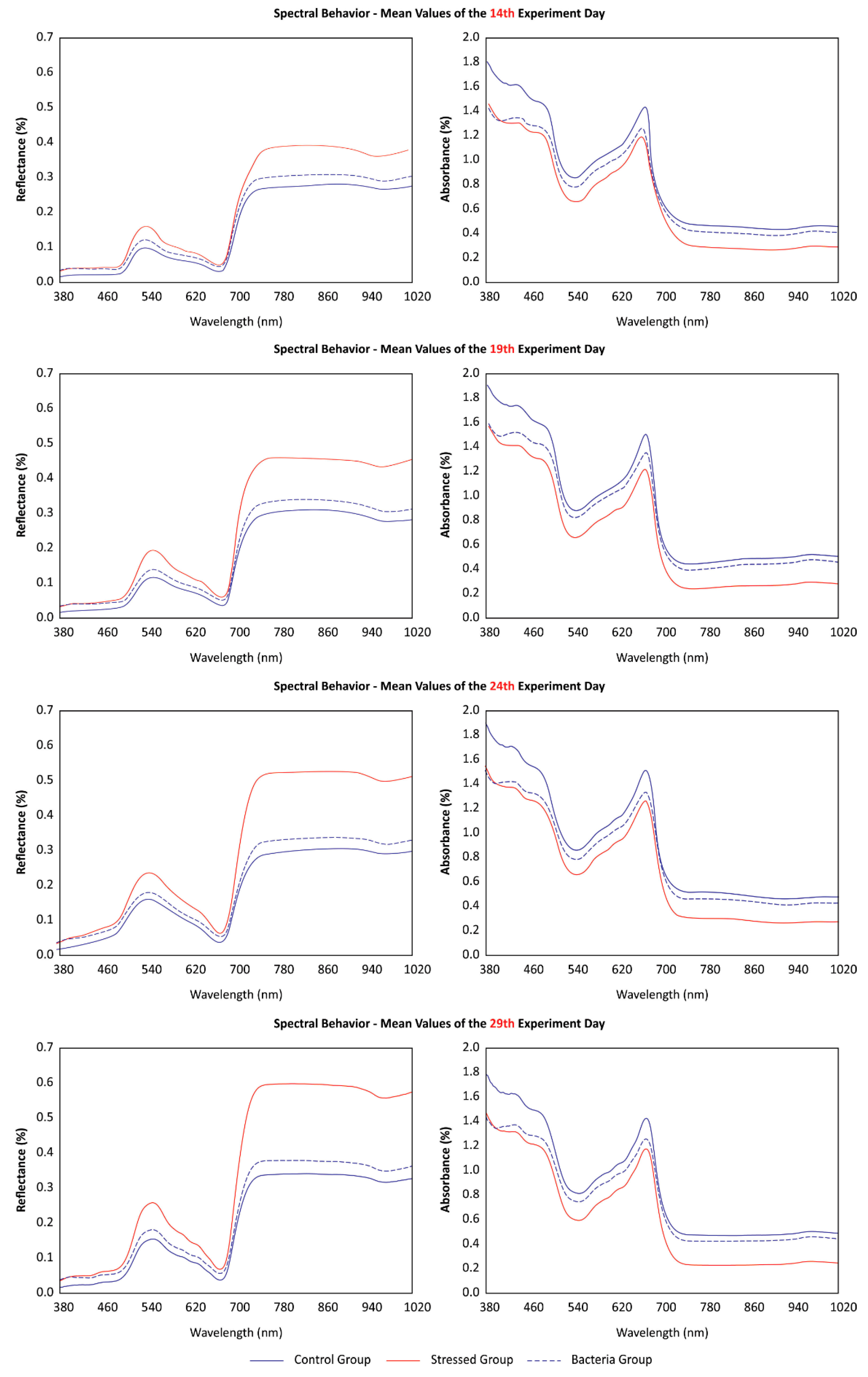
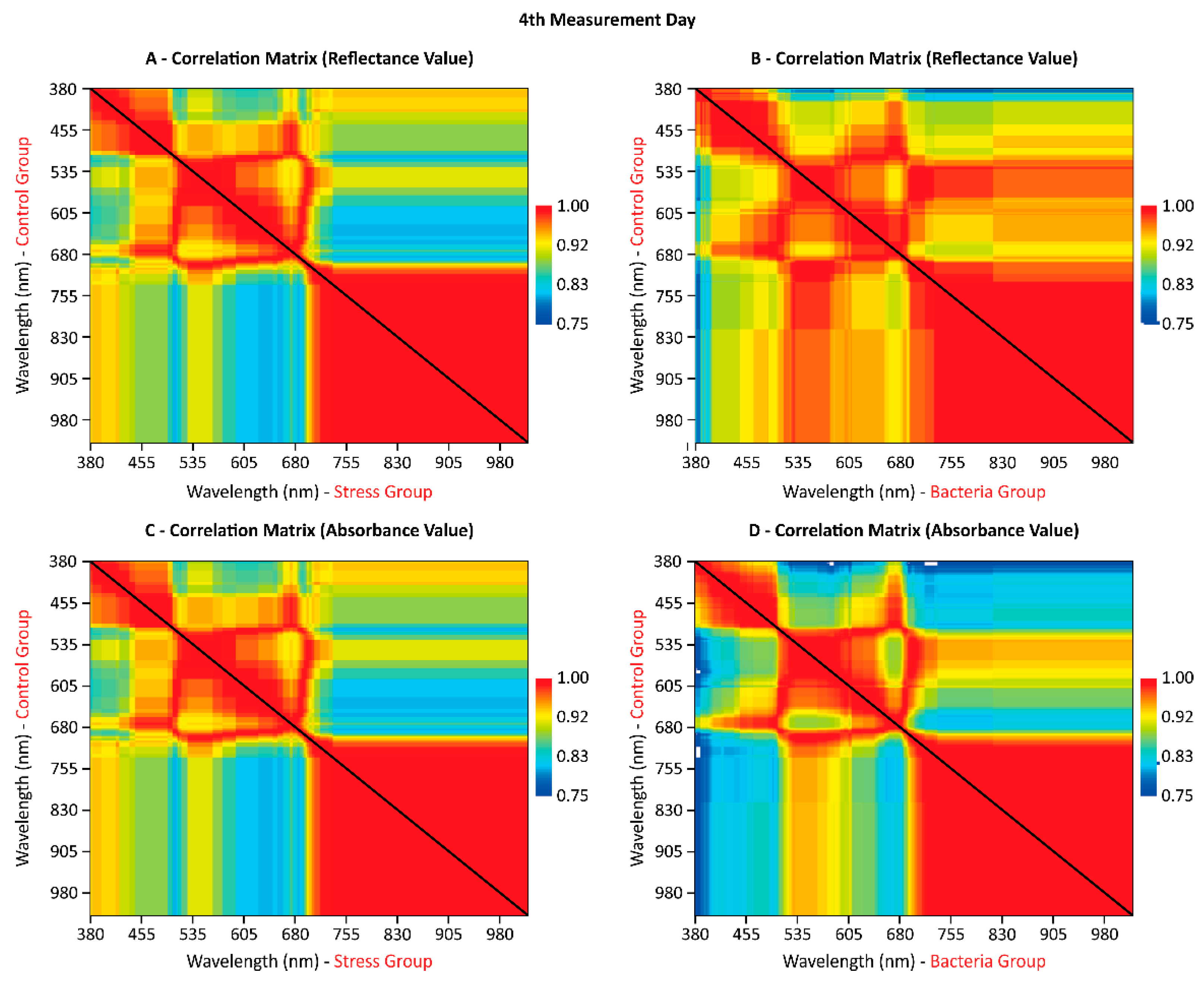
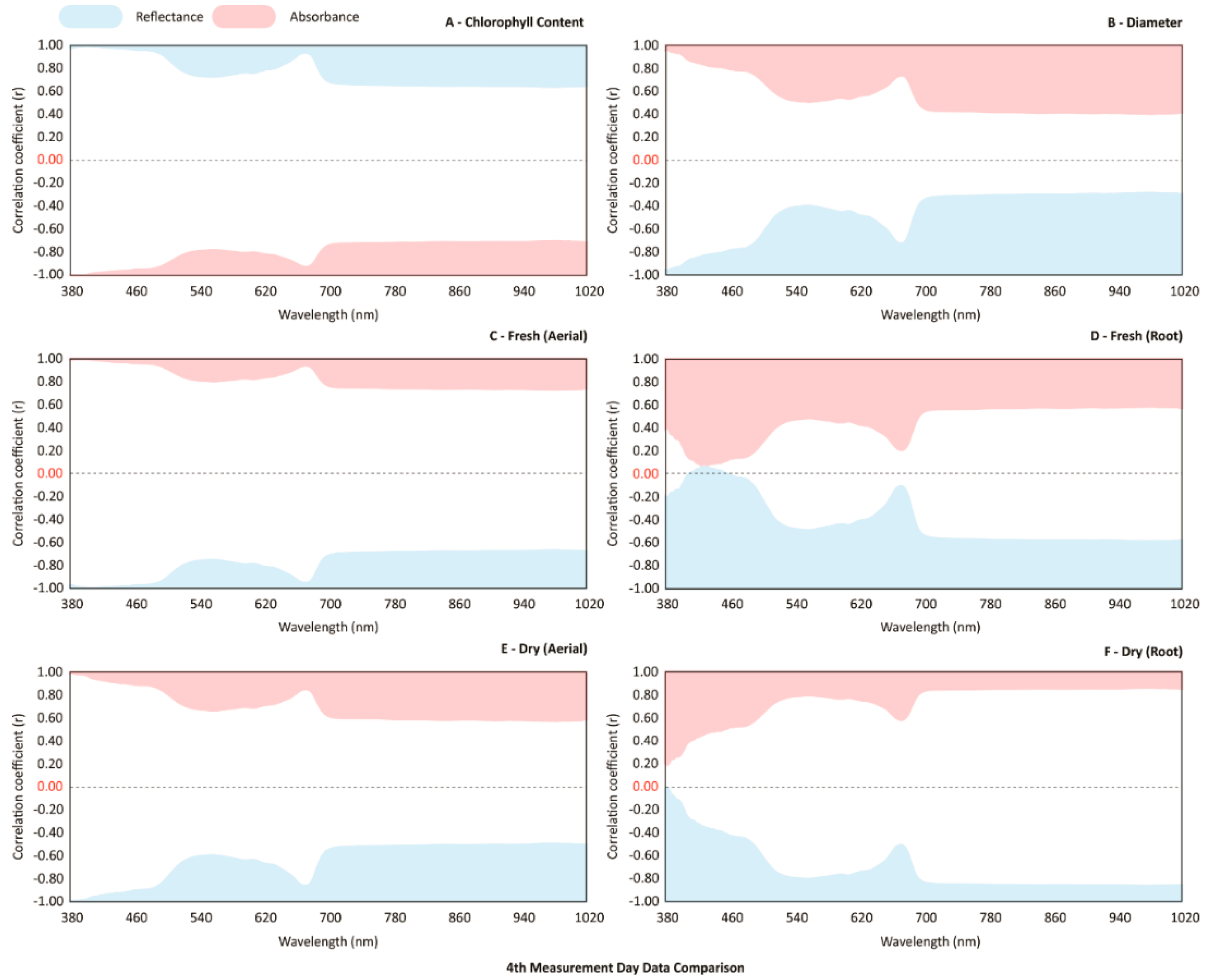
3.1. Hyperspectral and Biophysical Parameters Comparison

The water stress caused a reduction in practically all biophysical parameters. The exception was for the root development node treatment inoculated with the rhizobacteria. This indicates that the influence of the bacteria was more evident in the root system. The bacteria group had mean values similar or even higher to those found for the control group, both in the fresh mass and in the dry root (

Table 1. Results from the mean test between the biophysical parameters mean.

Treatment	Chlorophyll Content	Diameter (cm)	Weight (g)
			Fresh (Aerial)	Fresh (Root)	Dry (Aerial)	Dry (Root)
Control Group	12.55 b	18.33 a	11.04 a	3.48 bc	1.86 a	0.48 b
Stress Group	20.02 a	17.17 a	6.87 bc	2.97 c	1.49 ab	0.40 c
Bacteria Group	19.60 a	16.58 ab	7.27 b	4.82 a	1.43 b	0.52 ab
C. V.	29.54	16.15	28.14	26.48	22.18	20.07
F value	4.677	7.942	35.56	6.952	3.293	6.236
p-value	0.0124	0.0012	<0.0001	0.0021	0.0417	0.0036

Mean values followed by equal letters in lines do not present differences at 5% in the Turkey test. C. V. = coefficient of variation.

). Chlorophyll content also expressed high differences between the control group and the others.

At the end of the experiment, the lowest values of reflectance and the highest values of absorbance were observed in the control group (Figure 3). The spectral behavior of each treatment increased in difference as the stress progress continued. Stress and bacteria groups were both submitted to water stress, and their spectral response curves were distanced from the control curve. This condition can be explained by the reduction in fresh leaf mass and leaf diameter, which caused an increase in chlorophyll concentration in both groups (stress and bacteria). Furthermore, a continuous analysis over time showed that reflectance and absorbance values both increased and decreased, respectively. The stress group; however, was the one that presented a higher discrepancy over time.

To evaluate the correlation between each spectral behavior in the final day of the experiment, a matrix (Figure 4) was organized with the correlation values between all groups. In general, the control group presented better correlations with the bacteria group than the stress group. The correlation was higher in the near-infrared region for all curves. The green region (from 520 to 580 nm) was more evident on the reflectance curve in the bacteria group and was better isolated when evaluated on the absorbance curve (Figure 4C,D). This could prove difficult in differentiating both groups’ spectral behavior. Still, both groups returned different amplitudes in the averaged values (Figure 3), which indicates a feasible separation between them.

The relationship between the biophysical parameters and all the spectral wavelengths of the three groups is shown in Figure 5. The parameters that presented best correlations with the spectral curves were chlorophyll, fresh masses and aerial dry matter, and dry weight of roots. With the exception of the dry root weight, the aforementioned parameters presented higher negative and positive correlations in the visible region (Figure 5A,C,D), specifically in the blue region (from 380 to 460 nm) and in a smaller range in the red region (between 640 and 680 nm), which coincides with the absorption regions of chlorophyll. The weight of the root dry mass was the parameter that presented the highest correlation (r = 0.80) with the near-infrared region (700 nm onwards).

The mean values of the correlation of each parameter with the reflectance and absorbance curves were also compared (

Table 2. Differences from mean values to correlations from absorbance and reflectance.

Biophysical Parameter	Mean Correlation ± Std. Dev.		Mean Difference	R2	RMSE	R2	RMSE
	Reflectance (r)	Absorbance (r)		Reflectance		Absorbance
Chlorophyll Content	0.759 ± 0.131	−0.803 ± 0.104	1.562 (1.549–1.574)	0.43	0.125	0.70	0.102
Diameter	−0.486 ± 0.215	0.540 ± 0.175	1.026 (1.006–1.047)	0.11	0.128	0.38	0.180
Fresh Weight (Aerial)	−0.779 ± 0.122	0.822 ± 0.097	1.602 (1.591–1.613)	0.47	0.099	0.72	0.120
Fresh Weight (Root)	−0.421 ± 0.278	0.377 ± 0.228	0.797 (0,771–0.824)	0.36	0.108	0.17	0.209
Dry Weight (Aerial)	−0.646 ± 0.172	0.695 ± 0.139	1.341 (1.325–1.357)	0.27	0.116	0.56	0.152
Dry Weight (Root)	−0.734 ± 0.226	0.709 ± 0.186	1.443 (1.422–1.465)	0.76	0.065	0.47	0.166

): the chlorophyll, diameter, fresh aerial weight, and dry root weight had better correlations (r = −0.803; 0.540; 0.822; and 0.709, respectively) with absorbance than with reflectance. The difference between averages ranged from 0.797 (fresh root) to 1.602 (fresh aerial), which demonstrates how much the reflectance values differ from those of absorbance. This behavior is better observed in the absorbance wavelengths of chlorophyll, fresh weight of the aerial part and in the dry-root weight, which presented values higher than 0.7, and the lowest values in root mean squared error (RMSE).

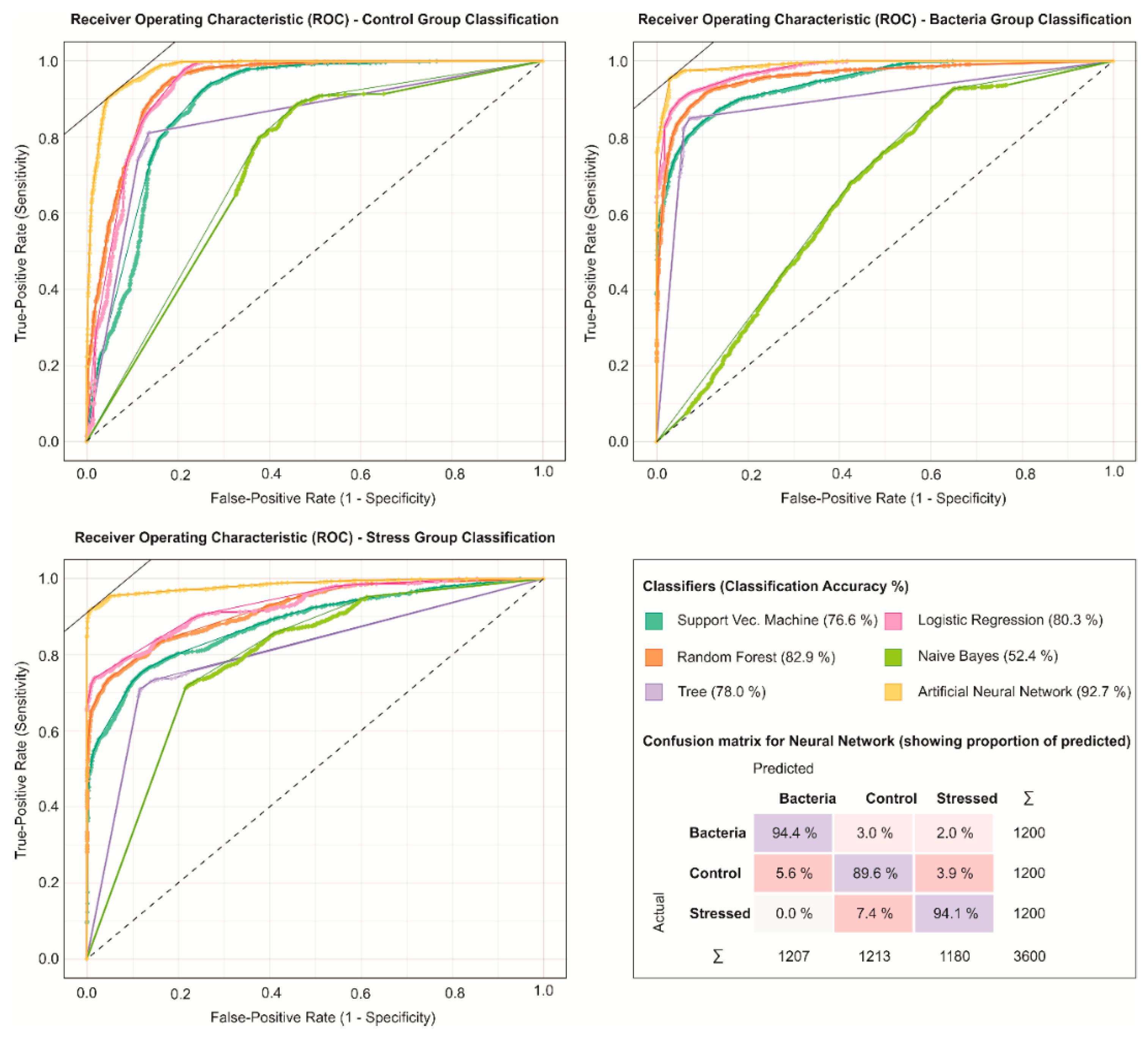
3.2. Modeling the Hyperspectral Wavelengths Through Artificial Neural Network

The wavelengths were modeled by different machine learning algorithms from the 14th day of the experiment. The ANN model presented here was able to classify better than any of the remaining algorithms since the first day of measurement (

Table 3. Accuracy metrics for each of the machine learning algorithms evaluated in this study.

Model	AUC		Class. Acc. (%)		F1-Score (%)		Precision (%)		Recall (%)
Day: 14th	Refl.	Abs.	Refl.	Abs.	Refl.	Abs.	Refl.	Abs.	Refl.	Abs.
Decision Tree	0.620	0.741	58.5	63.5	58.6	63.6	57.8	63.9	57.6	63.5
SVM	0.671	0.767	59.8	63.8	58.1	63.2	55.3	65.4	58.8	63.8
Random Forest	0.712	0.822	56.4	66.5	56.0	66.5	56.7	66.5	59.9	66.5
ANN	0.794	0.924	70.3	79.6	68.2	79.7	71.2	80.1	70.4	79.6
Naïve Bayes	0.589	0.707	44.2	54.8	46.4	54.2	49.8	55.4	50.1	54.8
Logistic Regression	0.701	0.833	66.2	71.4	60.3	71.3	65.4	71.4	61.9	71.4
Day: 19th	Refl.	Abs.	Refl.	Abs.	Refl.	Abs.	Refl.	Abs.	Refl.	Abs.
Decision Tree	0.702	0.772	60.5	69.2	59.5	69.2	64.6	69.3	60.2	69.2
SVM	0.755	0.803	58.8	60.6	59.2	58.0	58.4	60.6	58.8	60.6
Random Forest	0.811	0.891	62.3	74.5	56.5	74.5	64.0	74.5	69.2	74.5
ANN	0.904	0.941	75.6	82.0	70.8	81.9	74.1	81.8	74.0	82.0
Naïve Bayes	0.677	0.694	50.0	50.6	48.2	47.7	45.4	48.8	44.3	50.6
Logistic Regression	0.733	0.858	65.4	67.3	59.3	66.0	62.4	66.2	59.3	67.3
Day: 24th	Refl.	Abs.	Refl.	Abs.	Refl.	Abs.	Refl.	Abs.	Refl.	Abs.
Decision Tree	0.792	0.869	78.8	81.2	74.2	81.2	75.3	81.2	74.1	81.2
SVM	0.813	0.949	72.6	83.7	76.6	83.9	75.2	84.6	71.6	83.7
Random Forest	0.899	0.952	70.5	84.4	73.5	84.4	78.6	84.5	78.5	84.4
ANN	0.922	0.985	82.5	90.5	85.4	90.4	84.7	90.5	83.6	90.5
Naïve Bayes	0.684	0.869	60.2	70.4	67.9	70.7	65.8	71.4	61.4	70.4
Logistic Regression	0.868	0.971	77.9	89.4	76.1	89.3	67.8	89.4	72.1	89.4
Day: 29th	Refl.	Abs.	Refl.	Abs.	Refl.	Abs.	Refl.	Abs.	Refl.	Abs.
Decision Tree	0.818	0.845	81.2	78.0	71.3	78.0	70.2	78.0	64.9	78.0
SVM	0.879	0.902	83.7	76.6	70.2	76.8	71.7	77.5	62.3	76.6
Random Forest	0.912	0.942	84.4	83.1	74.5	83.1	75.3	83.7	70.1	83.1
ANN	0.945	0.984	90.5	92.7	81.3	92.7	82.4	92.7	79.3	92.7
Naïve Bayes	0.819	0.719	70.4	52.4	38.7	48.0	60.1	49.3	46.4	52.4
Logistic Regression	0.901	0.945	89.4	75.3	89.3	80.3	70.8	80.6	64.3	80.3

). In general, the absorbance values offered better accuracy than the reflectance ones. The accuracy and other metrics were improved with each measurement, indicating an increased difference over time.

The other machine learning algorithms were also able to return similar classification accuracies. The logistic regression method presented high accuracy in the first three measurements. However, it declined over the final day. This behavior was noted for the other algorithms as well. ANN was not only able to maintain consistency over time but also presented its highest accuracy on the final day. Another observation is that, to all machine learning methods applied here, the absorbance values were more efficient in discriminating the plant groups in most of the classifications.

To visualize the differences between each group, an ROC curve of the last day of measurement was used (Figure 6). The ROCs suggest that the ANN was better to differentiate individually the three groups, while other algorithms performed worse at specific conditions. The ANN also returned a less false-positive rate than all of the other machine learning algorithms. The confusion matrix of the final measurement day also shows how the ANN had more problems in predicting the control group (89.6%) than the other groups (94.4% and 94.1%, bacteria and stress, respectively).

Based on this classification, the gain ratio and the relief-F were used to evaluate the contribution of individual wavelengths to the ANN model (Figure 7). These metrics suggest that the stress group presented higher differences with the control group than the bacteria group, easily distinguishable by the algorithm. However, there appears to be a higher discrepancy between the bacteria group and the control group at the blue region (380 to 440 nm). Nonetheless, the near-infrared region and the 660 to 730 nm region appears to be contributing more to the stress group response.

4. Discussion

This study evaluated the spectral response of lettuce submitted to water stress while modeling its effects with an ANN and other machine learning algorithms. For that, we separated our data into three groups: control, stress, and bacteria. The reason to include the rhizobacteria in this situation is to induce a similarity with what transpires in greenhouses or horticulture models, as this bacterium is commonly present in soil and commercial seeds [29]. The addition of the bacteria group is also important to reinforce our test as it can act as a middle-ground between the stress group and the control group. We firstly evaluated the biological and physical response of the induced stress, and later compared it with the hyperspectral measurement. Lastly, we used ANN and other machine learning algorithms to classify both groups solely by their spectral response.

Our results indicate that the physiological response to water stress in early-stage lettuce is the reduction in leaf size and an increase in chlorophyll concentration. This behavior was evident both in the stress group and in the bacteria group, although with lower intensity in the latter. Changes in leaf pigmentation are noticeable in cases of plant stress [15]. However, an interesting observation is that the stress did not affect root weight in the bacteria group. This indicates that there is an effect in mitigating this stress, although this was not indicated by leaf analysis. By examining the mean spectral curves of each treatment (Figure 2) there is a small amplitude between the red-edge region wavelengths. The red-edge region is commonly known to indicate stress presence [23,34], and this may explain why the bacteria group did not differentiate much from the control group here.

Regarding the correlation between biophysical parameters and the wavelengths, it is initially perceived that absorbance wavelengths are more correlated with most biophysical parameters. An important observation to be made is the strongest correlation between chlorophyll and leaf fresh-weight with these wavelengths (Figure 4 and Table 2). This relationship between absorbance levels and the biophysical parameter was continuous throughout the experiment, particularly in regard to modeling each group’s response with machine learning algorithms (Table 3). Still, the correlation was more pronounced in the green and near-infrared regions (Figure 3). This situation is also evident when observing the mean curves of each treatment (Figure 2), where the amplitude between the curves is smaller in the blue, red, and red-edge remaining regions.

The classification performed by the ANN algorithm in this study showed interesting results since the first day of measurement when lettuces had just been stressed one day before the actual measurement. This condition is important to mention as it indicates how powerful hyperspectral analysis in conjunction with machine learning algorithms can be. From the evaluation metrics used in this study, it is evident how ANN was better in distinguishing the three plant groups. By observing the phenomenon temporally, one can see how the performance of the algorithms increased (Table 3). This can be explained by the increased distinction between the wavelengths of each group. As the stress occurred, the spectral behavior of these experiments became distinct from each other. Because this study is unique in this regard, there is a lack of literature to compare with. Still, the accuracy found here is similar to or even higher than those obtained by modeling different stresses effects in plants [21,24,25,26,27].

Another contribution of this study is the evaluation of the performance of different algorithms for both reflectance and absorbance wavelengths. Absorbance curves were directly related to changes in biophysical parameters for all treatments (Figure 4 and Table 2). This persisted in the machine learning analysis, where the performance of the algorithms was superior in differentiating the three groups by using their absorbance values. Thus, it is recommended that the modeling of these effects in lettuce is preferably performed from the conversion of reflectance to absorbance data. Another observation is that, by evaluating the performance of each algorithm over time, the ANN accuracy reached its peak at the last measurement day (with 92.7%), while the other algorithms decreased in performance (from the third to the fourth day of evaluation). This indicates how feasible the ANN algorithm was in modeling the water-stress effects in comparison to the others.

Lastly, the ANN algorithm has shown high precision and recall values (Table 2) when classifying each group, as shown in Figure 5. The confusion matrix demonstrated a small decrease in performance (89.6%) for differentiating the control group from the others. Regardless, the gain ratio and relief-F metrics (Figure 6) show how each individual wavelength contributed to the ANN model. In the gain ratio analysis, there is a predominance of wavelengths in the region of blue (380 to 440 nm), red (660 to 730 nm), and near-infrared (790 nm onwards). Despite the similarity between the curves of both groups, there was a smaller amplitude difference for the blue region. This may indicate how much the blue region contributed to differentiate the effects of the stress on the bacteria group. This was similar in the assessment of relief-F curves, in which this same region presented an even higher value than the group under stress. The blue region is responsible for the absorption of chlorophyll and may be an indication of how important the stress effect was in this spectral range. Nevertheless, the model also indicated greater contributions in the red region, red-edge, and near-infrared, which corroborates with the observations made during previous results (Figure 3). Apart from other species and cultivars, future research could be conducted exploring additional spectral regions such as the shortwave infrared (SWIR) region that is unfortunately not considered in the Fieldspec HandHeld ASD spectroradiometer device.

5. Conclusions

In this study, we have applied an artificial neural network algorithm to model the hyperspectral response of water-induced stress in lettuce. The ANN algorithm detected differences since the first day of the induced stress, with an 80% classification accuracy. The algorithm continued to present an increasing performance along with time-series analysis, resulting in a final 93% accuracy. The spectral wavelengths that contributed the most for its prediction were located around 380 to 440 nm, 660 to 730 nm, and, on a lower level, 790 nm onwards. We also detected that absorbance values are more suitable to deal with this issue than reflectance. Although the rhizobacteria did mitigate the water-stress effect at some point, a spectral behavior difference was noticed by the ANN algorithm, proving its robustness. The proposed approach indicated how feasible water stress in lettuce at early stages is measurable with machine learning algorithms such as ANN in hyperspectral data. While the small number of instances (four measurement days) evaluated could provide problems for the experiment, all machine learning algorithms tested here were able to classify it appropriately. For future works, we recommend similar studies with other species and cultivars. Additionally, the method demonstrated here could be scaled up to remote sensing platforms like unmanned aerial vehicles (UAV), as currently hyperspectral sensors can be embedded in it.

References

1. Díaz-Varela, R.A.; de la Rosa, R.; León, L.; Zarco-Tejada, P.J. High-resolution airborne UAV imagery to assess olive tree crown parameters using 3D photo reconstruction: Application in breeding trials. Remote Sens. 2015, 7, 4213–4232. [Google Scholar] [CrossRef]
2. Ampatzidis, Y.; Partel, V. UAV-based high throughput phenotyping in citrus utilizing multispectral imaging and artificial intelligence. Remote Sens. 2019, 11, 410. [Google Scholar] [CrossRef]
3. Chen, J.; Li, F.; Wang, R.; Fan, Y.; Raza, M.A.; Liu, Q.; Yang, W. Estimation of nitrogen and carbon content from soybean leaf reflectance spectra using wavelet analysis under shade stress. Comput. Electron. Agric. 2019, 156, 482–489. [Google Scholar] [CrossRef]
4. Muñoz-Huerta, R.F.; Guevara-Gonzalez, R.G.; Contreras-Medina, L.M.; Torres-Pacheco, I.; Prado-Olivarez, J.; Ocampo-Velazquez, R.V. A review of methods for sensing the nitrogen status in plants: Advantages, disadvantages and recent advances. Sensors 2013, 13, 10823–10843. [Google Scholar] [CrossRef]
5. Zhai, Y.; Cui, L.; Zhou, X.; Gao, Y.; Fei, T.; Gao, W. Estimation of nitrogen, phosphorus, and potassium contents in the leaves of different plants using laboratory-based visible and near-infrared reflectance spectroscopy: Comparison of partial least-square regression and support vector machine regression methods. Int. J. Remote Sens. 2013, 34, 2502–2518. [Google Scholar] [CrossRef]
6. Moharana, S.; Dutta, S. Spatial variability of chlorophyll and nitrogen content of rice from hyperspectral imagery. J. Photogramm. Remote Sens. 2016, 122, 17–29. [Google Scholar] [CrossRef]
7. Osco, L.P.; Ramos, A.P.M.; Moriya, É.A.S.; de Souza, M.; Junior, J.M.; Matsubara, E.T.; Imai, N.N.; Creste, J.E. Improvement of leaf nitrogen content inference in Valencia-orange trees applying spectral analysis algorithms in UAV mounted-sensor images. Int. J. Appl. Earth Obs. Geoinf. 2019, 83, 101907. [Google Scholar] [CrossRef]
8. Martins, G.D.; Galo ML, B.T.; Vieira, B.S. Detecting and mapping root-knot nematode infection in coffee crop using remote sensing measurements. IEEE J. Sel. Top. Appl. Earth Obs. Remote Sens. 2017, 10, 5395–5403. [Google Scholar] [CrossRef]
9. Kross, A.; McNairn, H.; Lapen, D.; Sunohara, M.; Champagne, C. Assessment of RapidEye vegetation indices for estimation of leaf area index and biomass in corn and soybean crops. Int. J. Appl. Earth Obs. Geoinf. 2015, 34, 235–248. [Google Scholar] [CrossRef]
10. Krishna, G.; Sahoo, R.N.; Singh, P.; Bajpai, V.; Patra, H.; Kumar, S.; Sahoo, P.M. Comparison of various modeling approaches for water-deficit stress monitoring in rice crop through hyperspectral remote sensing. Agric. Water Manag. 2019, 213, 231–244. [Google Scholar] [CrossRef]
11. Loggenberg, K.; Strever, A.; Greyling, B.; Poona, N. Modeling water stress in a Shiraz vineyard using hyperspectral imaging and machine learning. Remote Sens. 2018, 10, 202. [Google Scholar] [CrossRef]
12. Elvanidi, A.; Katsoulas, N.; Ferentinos, K.; Bartzanas, T.; Kittas, C. Hyperspectral machine vision as a tool for water stress severity assessment in soilless tomato crop. Biosyst. Eng. 2018, 165, 25–35. [Google Scholar] [CrossRef]
13. Lisar, S.Y.; Motafakkerazad, R.M.M.; Rahm, I.M. Water Stress in Plants: Causes, Effects, and Responses. Water Stress 2012, 10, 1–16. [Google Scholar] [CrossRef]
14. Gerhards, M.; Schlerf, M.; Rascher, U.; Udelhoven, T.; Juszczak, R.; Alberti, G.; Inoue, Y. Analysis of airborne optical and thermal imagery for detection of water stress symptoms. Remote Sens. 2018, 10, 1139. [Google Scholar] [CrossRef]
15. Maimaitiyiming, M.; Ghulam, A.; Bozzolo, A.; Wilkins, J.L.; Kwasniewski, M.T. Early detection of plant physiological responses to different levels of water stress using reflectance spectroscopy. Remote Sens. 2017, 9, 745. [Google Scholar] [CrossRef]
16. Delloye, C.; Weiss, M.; Defourny, P. Retrieval of the canopy chlorophyll content from Sentinel-2 spectral bands to estimate nitrogen uptake in intensive winter wheat cropping systems. Remote Sens. Environ. 2018, 216, 245–261. [Google Scholar] [CrossRef]
17. Kalacska, M.; Lalonde, M.; Moore, T.R. Estimation of foliar chlorophyll and nitrogen content in an ombrotrophic bog from hyperspectral data: Scaling from leaf to image. Remote Sens. Environ. 2015, 169, 270–279. [Google Scholar] [CrossRef]
18. Min, M.; Lee, W. Determination of significant wavelengths and prediction of nitrogen content for citrus. Am. Soc. Agric. Eng. 2005, 48, 455–461. [Google Scholar] [CrossRef]
19. Huang, W.; Lu, J.; Ye, H.; Kong, W.; Mortimer, A.H.; Shi, Y. Quantitative identification of crop disease and nitrogen-water stress in winter wheat using continuous wavelet analysis. Int. J. Agric. Biol. Eng. 2018, 11, 145–152. [Google Scholar] [CrossRef]
20. Zarco-Tejada, P.; González-Dugo, V.; Berni, J. Fluorescence, temperature and narrow-band indices acquired from a UAV platform for water stress detection using a micro-hyperspectral imager and a thermal camera. Remote Sens. Environ. 2012, 117, 322–337. [Google Scholar] [CrossRef]
21. Rocha, A.D.; Groen, T.A.; Skidmore, A.K. Spatially-explicit modelling with support of hyperspectral data can improve prediction of plant traits. Remote Sens. Environ. 2019, 231, 111200. [Google Scholar] [CrossRef]
22. Ghamisi, P.; Plaza, J.; Chen, Y.; Li, J.; Plaza, A.J. Advanced spectral classifiers for hyperspectral images: A review. IEEE Geosci. Remote Sens. Mag. 2017, 5, 8–32. [Google Scholar] [CrossRef]
23. Index, S.; Xu, N.; Tian, J.; Tian, Q.; Xu, K.; Tang, S. Analysis of vegetation red edge with different illuminated/shaded canopy proportions and to construct normalized difference canopy. Remote Sens. 2019, 11, 1192. [Google Scholar] [CrossRef]
24. Gao, J.; Meng, B.; Liang, T.; Feng, Q.; Ge, J.; Yin, J.; Wu, C.; Cui, X.; Hou, M.; Liu, J.; et al. Modeling alpine grassland forage phosphorus based on hyperspectral remote sensing and a multi-factor machine learning algorithm in the east of Tibetan Plateau, China. ISPRS J. Photogramm. Remote Sens. 2019, 147, 104–117. [Google Scholar] [CrossRef]
25. Zhang, J.; Huang, Y.; Reddy, K.N.; Wang, B. Assessing crop damage from dicamba on non-dicamba-tolerant soybean by hyperspectral imaging through machine learning. Pest Manag. Sci. 2019. [Google Scholar] [CrossRef]
26. Abdulridha, J.; Batuman, O.; Ampatzidis, Y. UAV-based remote sensing technique to detect citrus canker disease utilizing hyperspectral imaging and machine learning. Remote Sens. 2019, 11, 1373. [Google Scholar] [CrossRef]
27. Karadağ, K.; Tenekeci, M.E.; Taşaltın, R.A. Detection of pepper fusarium disease using machine learning algorithms based on spectral reflectance. Sustain. Comput. Inform. Syst. 2019. [Google Scholar] [CrossRef]
28. Fu, P.; Meacham-Hensold, K.; Guan, K.; Bernacchi, C.J. Hyperspectral leaf reflectance as proxy for photosynthetic capacities: An ensemble approach based on multiple machine learning algorithms. Front. Plant Sci. 2019. [Google Scholar] [CrossRef]
29. Enebe, M.C.; Babalola, O.O. The influence of plant growth-promoting rhizobacteria in plant tolerance to abiotic stress: A survival strategy. Appl. Microbiol. Biotechnol. 2018, 102, 7821–7835. [Google Scholar] [CrossRef]
30. Wang, J.; Xu, R.; Yang, S. Estimation of plant water content by spectral absorption features centered at 1,450 nm and 1,940 nm regions. Environ. Monit. Assess. 2008, 157, 459–469. [Google Scholar] [CrossRef]
31. Araujo, F.F.; Henning, A.A.; Hungria, M. Phytohormones and antibiotics produced by Bacillus subtilis and their effects on seed pathogenic fungi and on soybean root development. World J. Microbiol. Biotechnol. 2005, 21, 1639–1645. [Google Scholar] [CrossRef]
32. Anderson, K.; Rossini, M.; Labrador, J.P.; Balzarolo, M.; Arthur, A.; Fava, F.; Julitta, T. Vescovo. Inter-comparison of hemispherical conical reflectance factors (HCRF) measured with four fiber-based spectrometers. Remote Sens. Sens. 2013, 21, 605–617. [Google Scholar] [CrossRef]
33. FALKER. ClorofiLOGElectronic: Chlorophyll Content Meter. Available online: http://www.falker.com.br/en/product-clorofilog-chlorophyll-meter.php (accessed on 30 November 2018).
34. Liang, L.; Di, L.; Huang, T.; Wang, J.; Lin, L.; Wang, L.; Yang, M. Estimation of leaf nitrogen content in wheat using new hyperspectral indices and a random forest regression algorithm. Remote Sens. 2018, 10, 1940. [Google Scholar] [CrossRef] [Green Version]
35. Thomas, M. Mitchell. In Machine Learning, 1st ed.; McGraw-Hill, Inc.: New York, NY, USA, 1997. [Google Scholar]
Figure 1. The workflow of the experimental analysis conducted in this study.
Remotesensing 11 02797 g001
Figure 2. Example of the training curve with the difference in accuracy for the artificial neural networks (ANN) model.
Remotesensing 11 02797 g002
Figure 3. Comparison between the mean spectral reflectance and absorptance at selected wavelengths for each of the three treatment groups.
Remotesensing 11 02797 g003
Figure 4. The correlation matrix between the mean spectral wavelengths.
Remotesensing 11 02797 g004
Figure 5. The correlation coefficient (r) between the spectral wavelengths (380–1020 nm) and the biophysical parameter; reflectance (blue curve) and absorbance (pink curve).
Remotesensing 11 02797 g005
Figure 6. Receiver operating characteristic (ROC) curve comparison for each group classification and the ANN confusion matrix.
Remotesensing 11 02797 g006
Figure 7. The individual contribution of the wavelengths to model the water-stress induced lettuces in relation to the control group.
Remotesensing 11 02797 g007