Feasibility Study of Tractor-Test Vehicle Technique for Practical Structural Condition Assessment of Beam-Like Bridge Deck


Abstract
1. Introduction
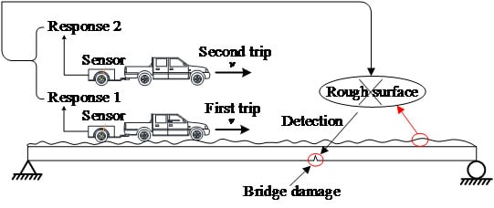
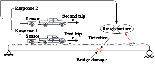
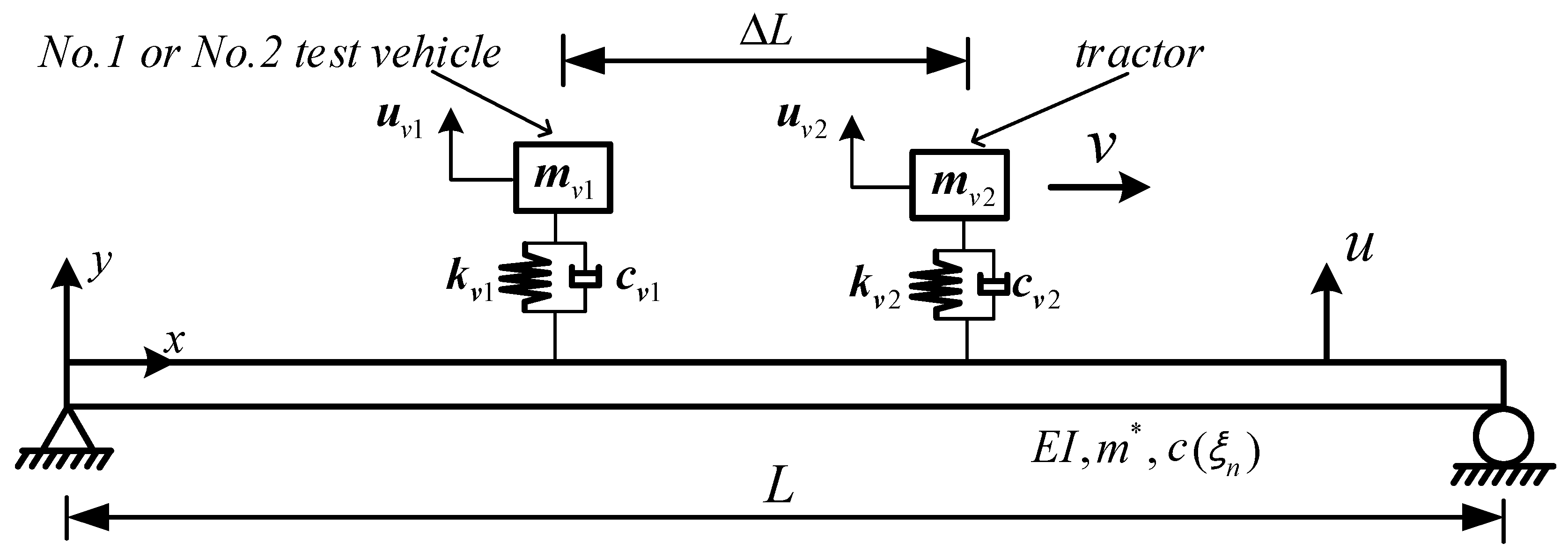
2. The Tractor-Test Vehicle Technique (TTVT) of Non-Destructive Testing
2.1. Indirect Measurement of Mode Shape of Bridge Structures
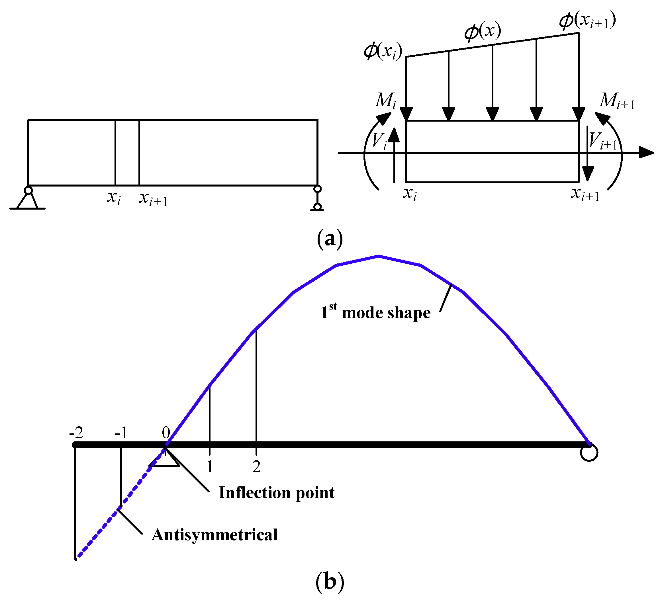
2.2. Element Bending Stiffness of Beam from the Improved DSC Method
2.3. Reducing the Effect of Road Surface Roughness
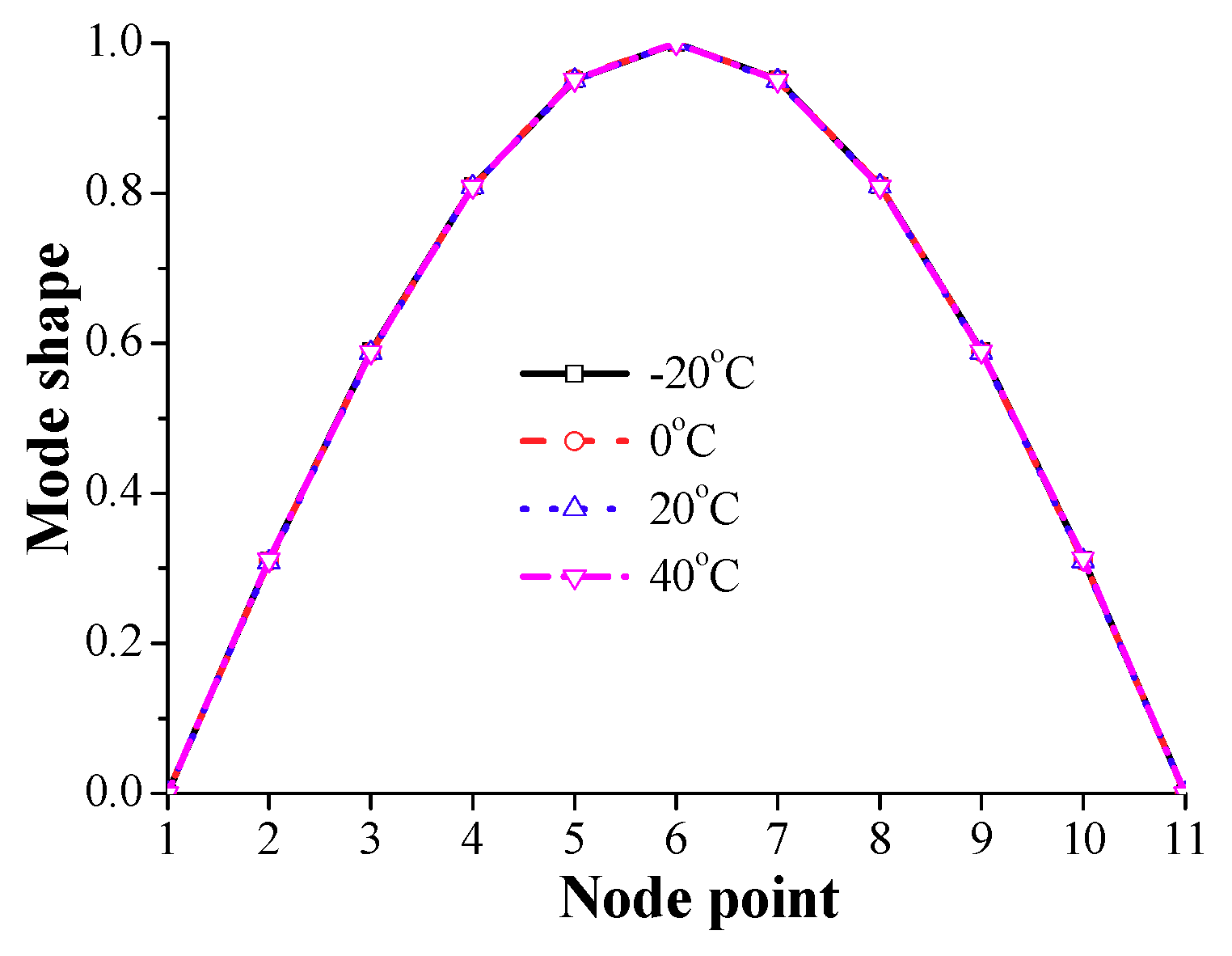
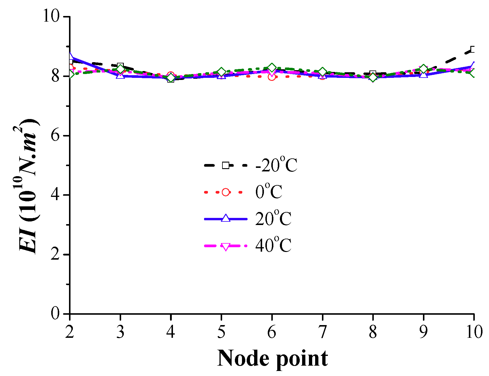
2.4. Effect of Ambient Temperature
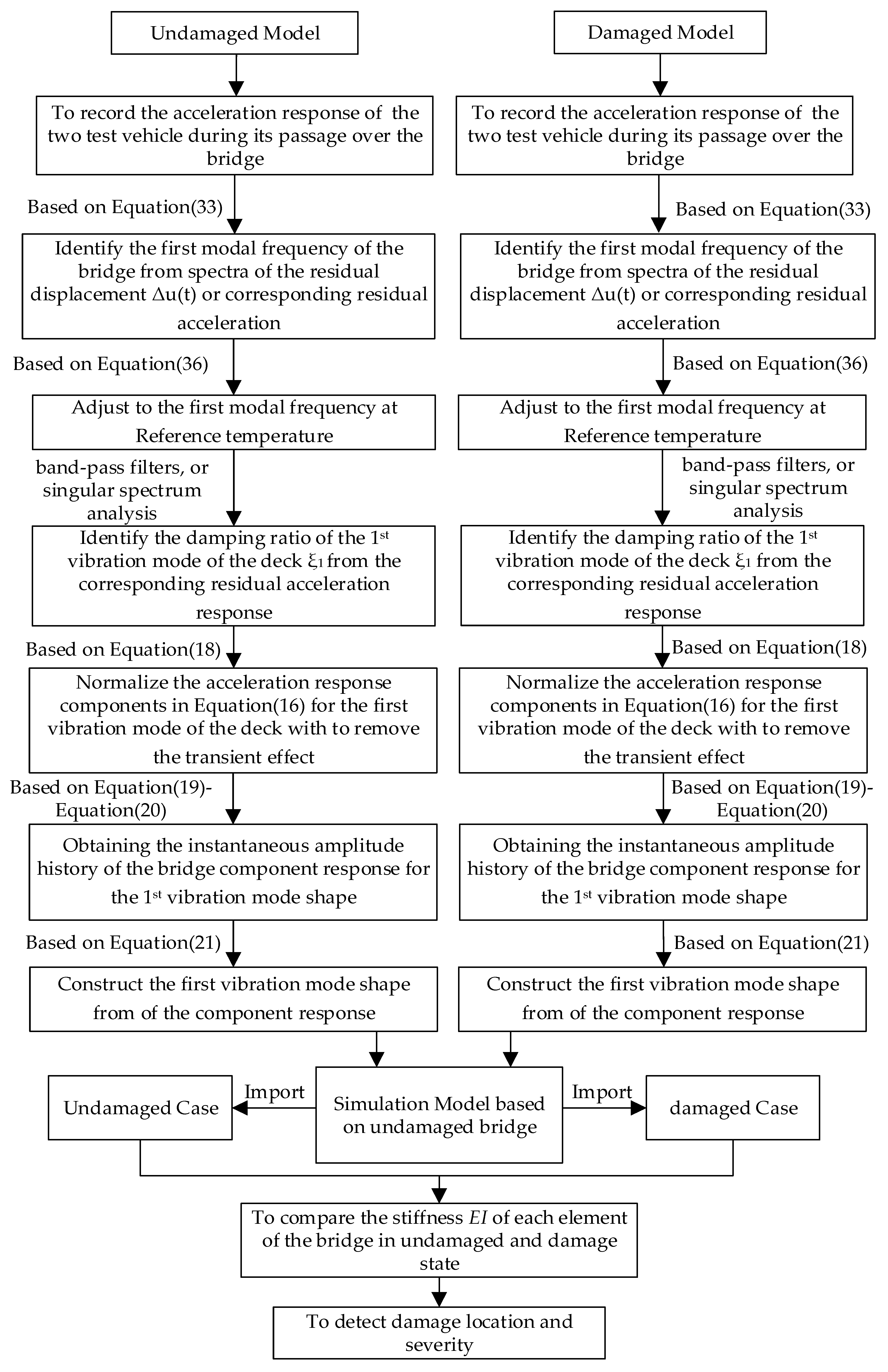
2.5. Analysis Procedure of Tractor-Test Vehicle Technique for Non-Destructive Testing
- (1)
- Record the acceleration responses of the two test vehicles in the undamaged state.
- (2)
- Identify the first modal frequency of the bridge structure from spectra of the residual displacement and corresponding residual acceleration , which indicate a vehicle response without the effect ofroad surface roughness based on tractor-test vehicle technique, in both the undamaged and damaged states of the structure. If the ambient temperature is different from the reference temperature, adjust the identified frequencies in both states to that at the reference temperature with Equation (36).
- (3)
- Normalize the acceleration response components in Equation(16) for the first vibration mode of the deck with to remove the transient effect. After the 1st bridge frequency is made available, one can extract the acceleration response components and the damping ratio of the 1st vibration mode of the deckassociated with from the corresponding residual accelerationby any feasible signal processing tools.
- (4)
- Then, obtaining the instantaneous amplitude history of the bridge component response for the 1st vibration mode shape. Performing the Hilbert transform to the decomposed bridge component response in Equation (18) yields its transform pair in Equation (19). Then, one can obtain the instantaneous amplitude history of the bridge component response using Equations (20) and (21).
- (5)
- Construct the first vibration mode shape from of the component response by Equation (21), the curve of the instantaneous amplitude function is representative of the mode shape of the bridge in absolute value. The sign of the 1st mode shape can be decided according to engineers’ judgment or experience [9].
- (6)
- Calculate the modal curvature of the beam using the mode shape obtained above by the central difference method with due correction described in Section 3.
- (7)
- Calculate the bending moment M of the beam with Equation (23) for each monitored cross-section of the deck.
- (8)
- Calculate the bending stiffness EI of the beam using Equation (22) for each monitored cross-section of the deck.
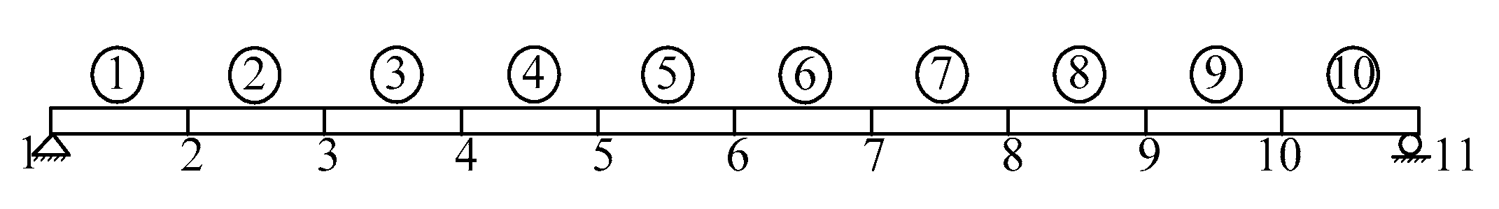
3. Numerical Study
3.1. Ratio of Vehicle Parameters
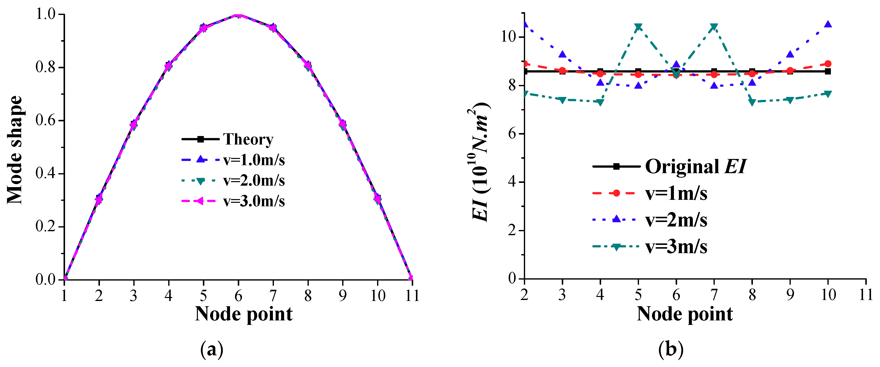
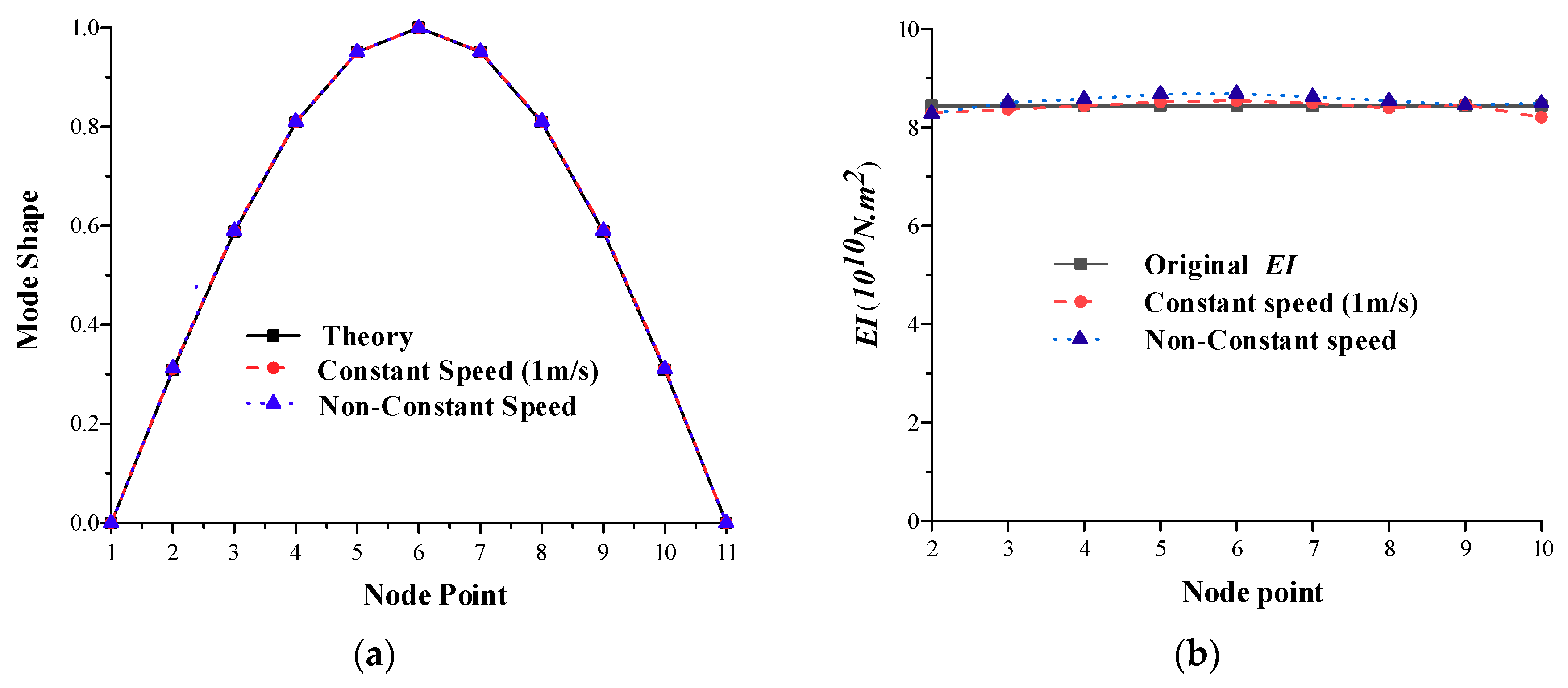
3.2. Effect of Constant Vehicle Speed
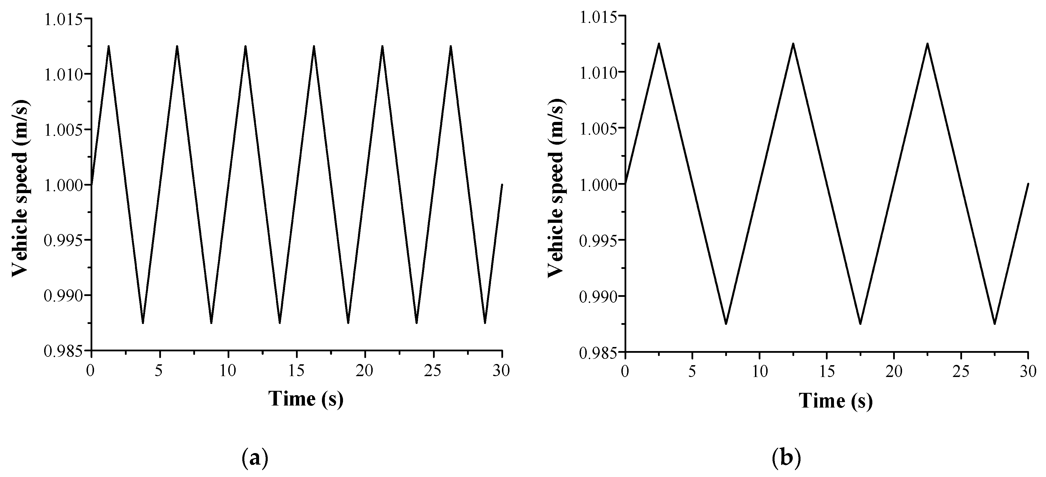
3.3. Effect of Non-Constant Vehicle Speed
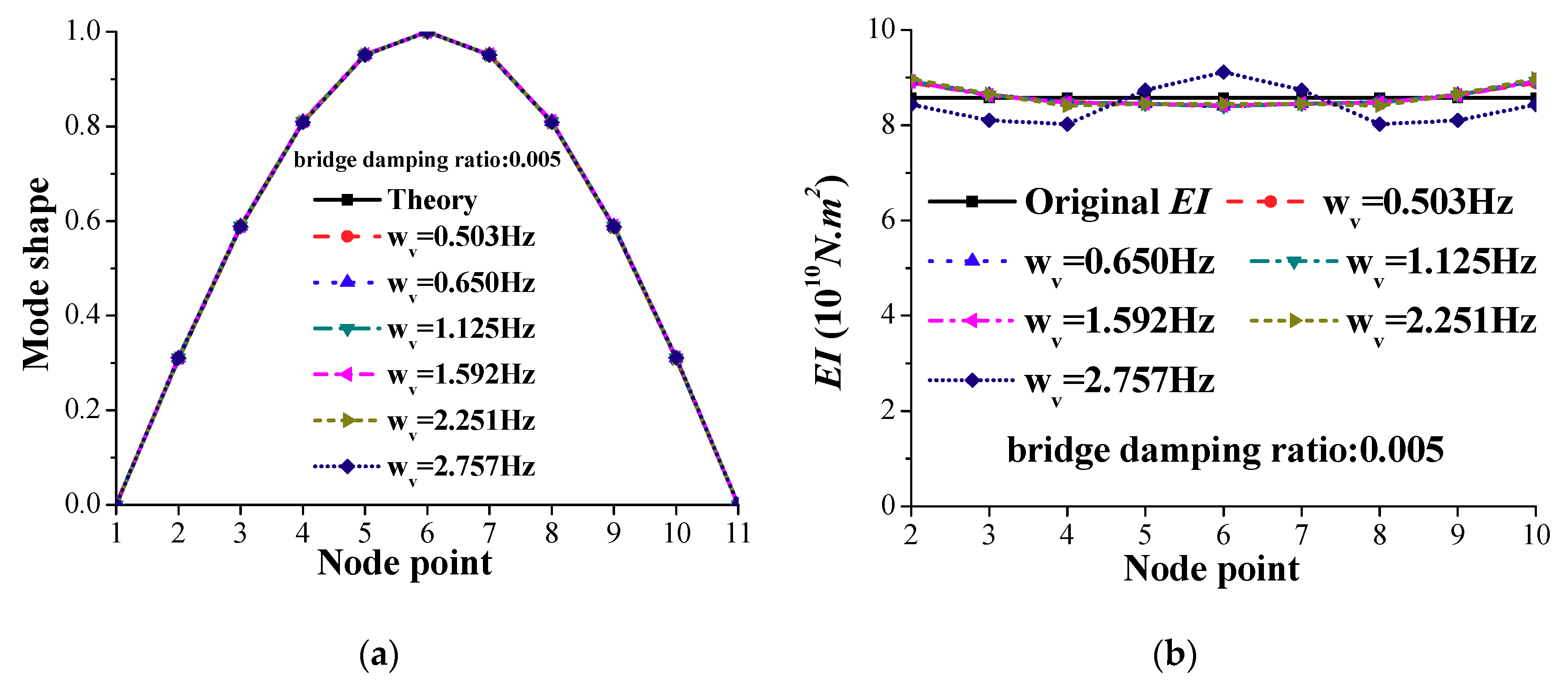
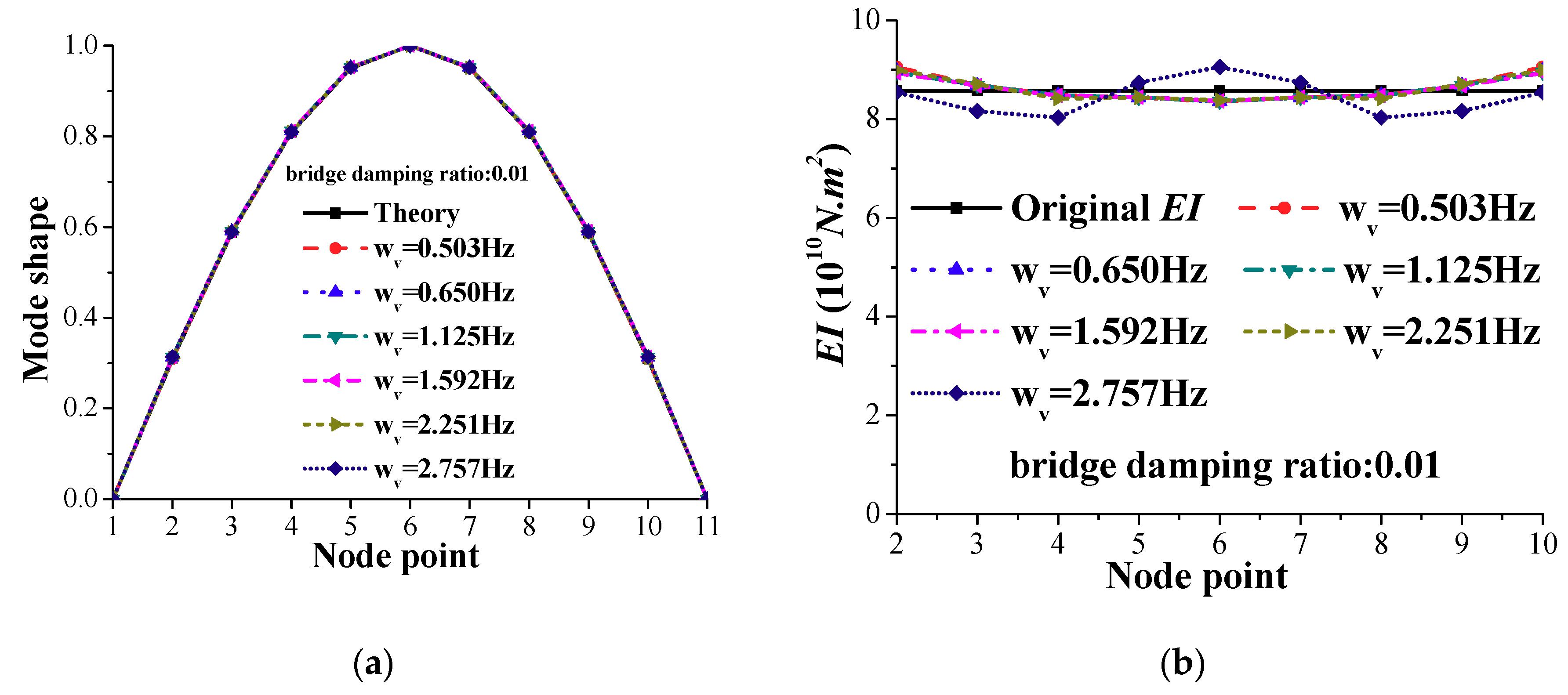
3.4. Effect of Vehicle Modal Frequency
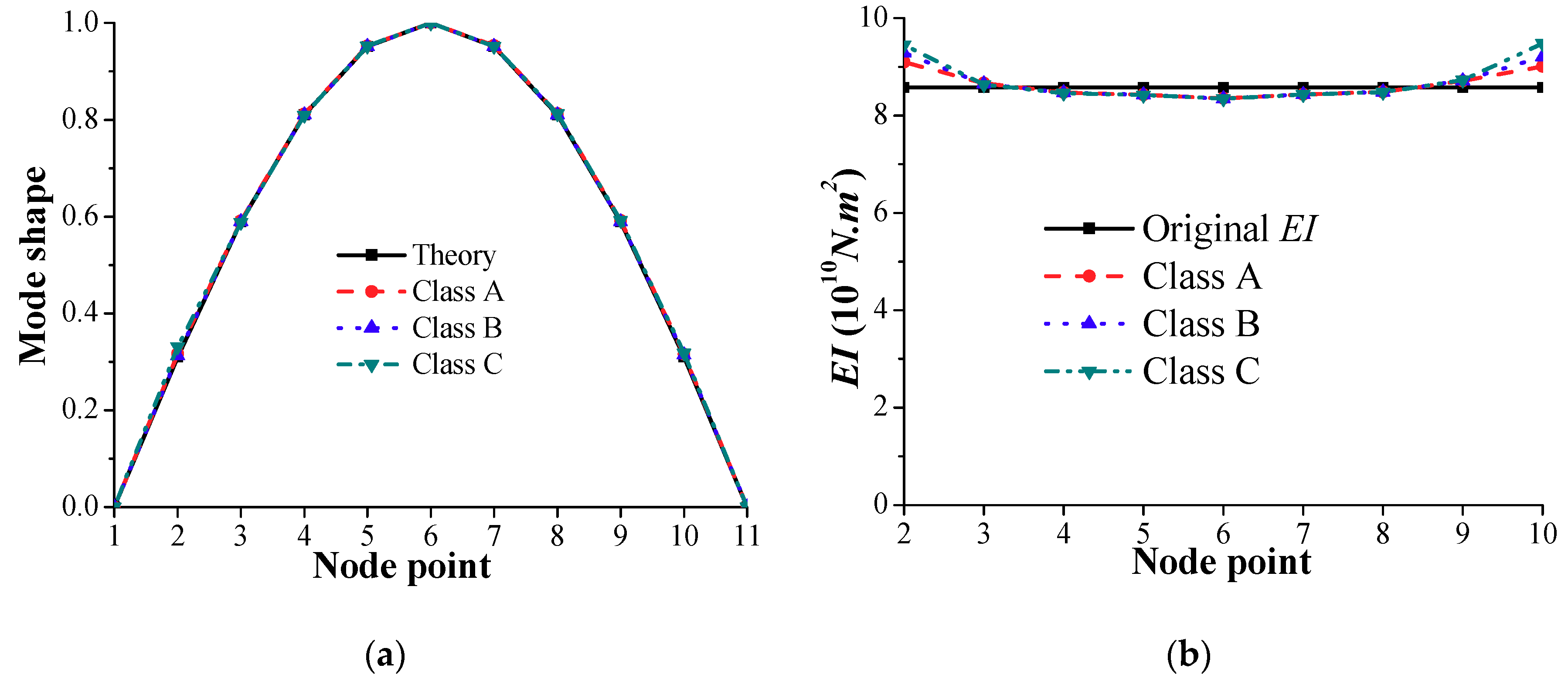
3.5. Effect of Road Surface Roughness
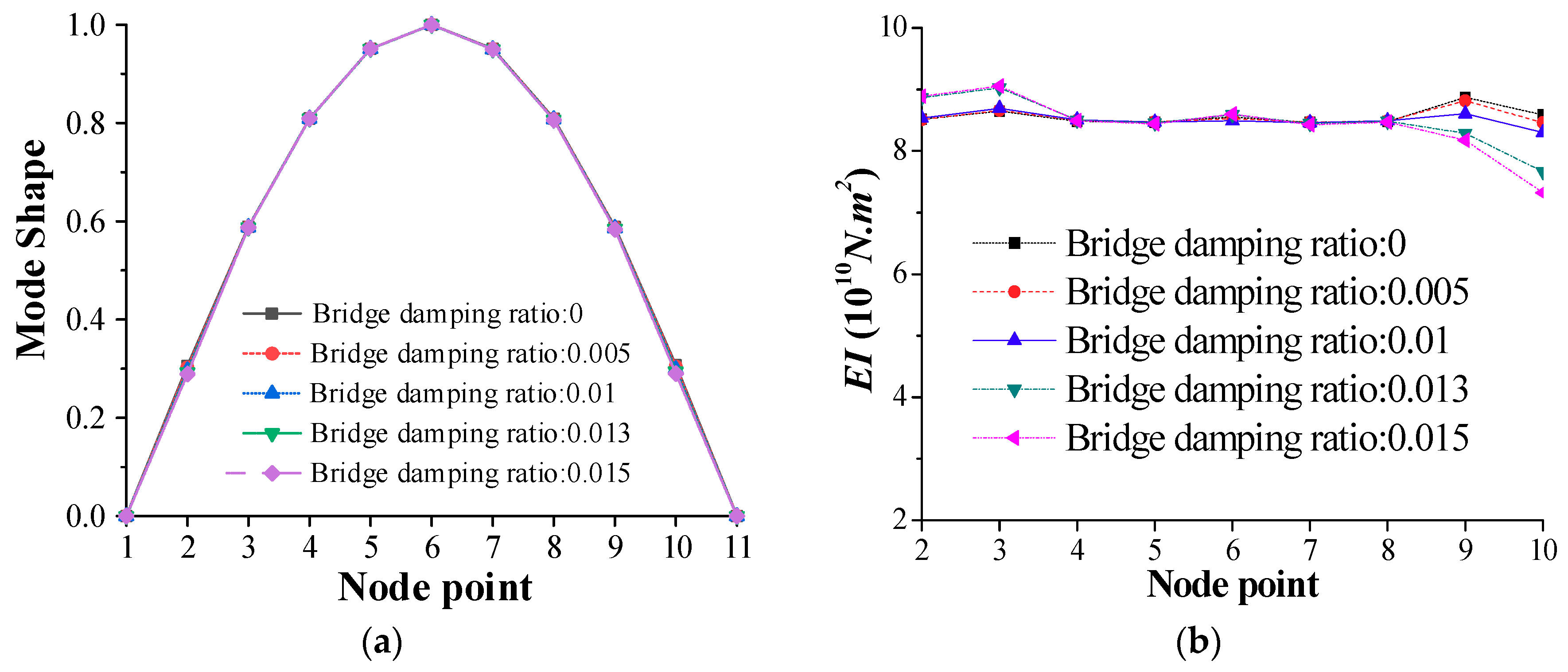
3.6. Effect of Bridge Damping Ratio
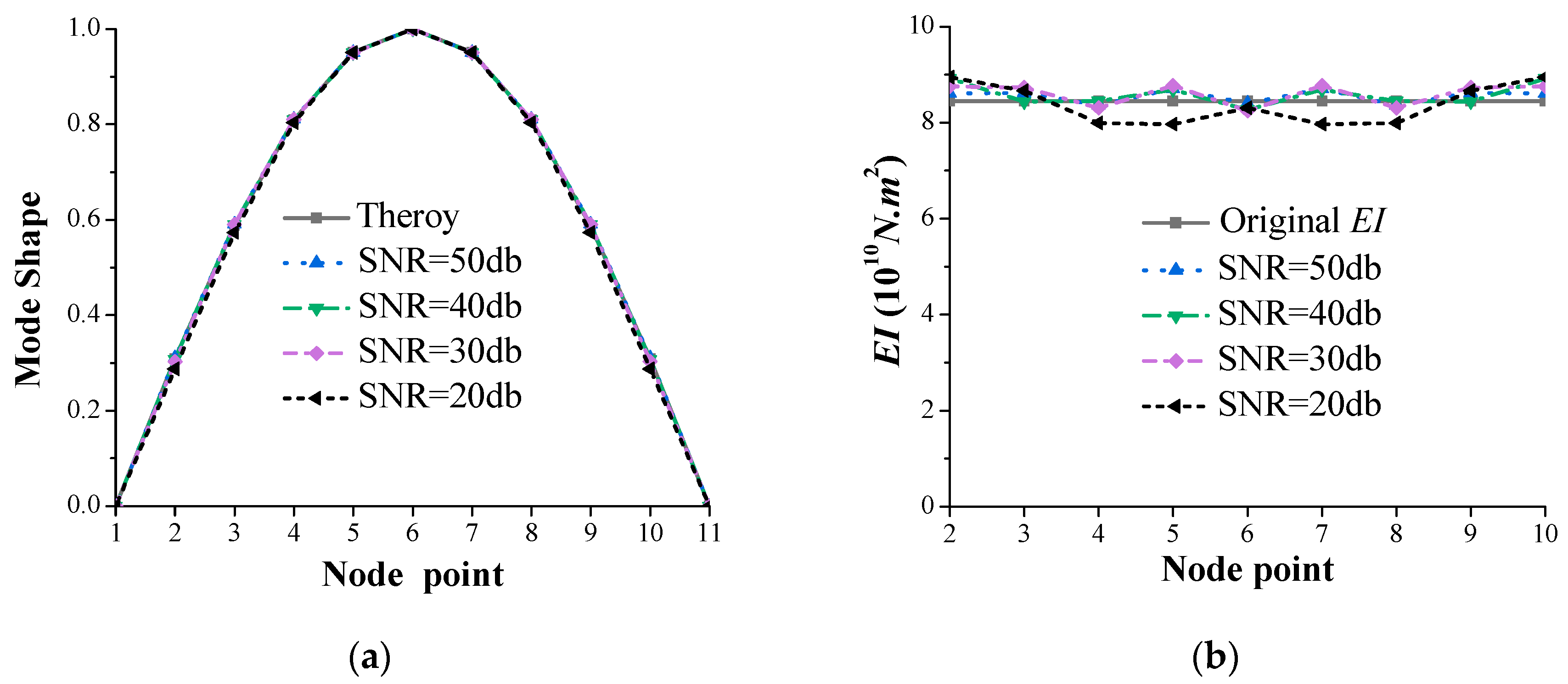
3.7. Effect of Measurement Noise
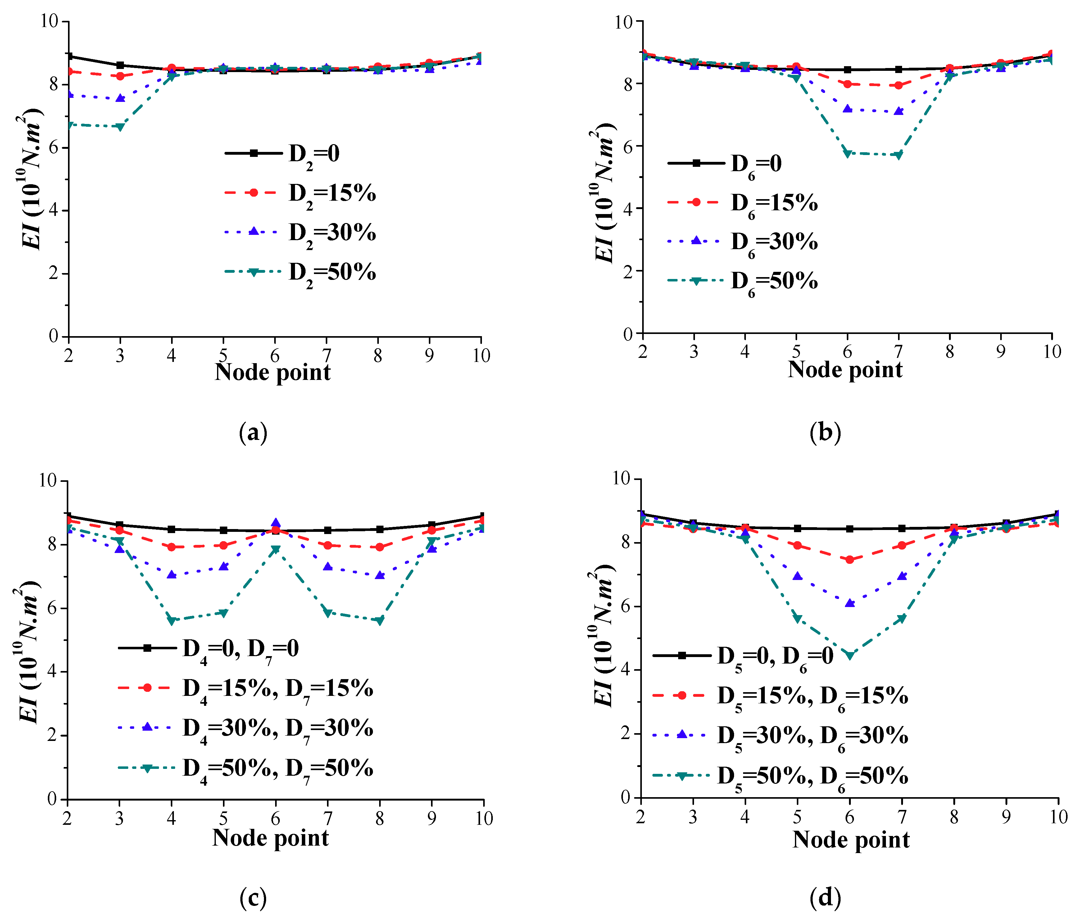
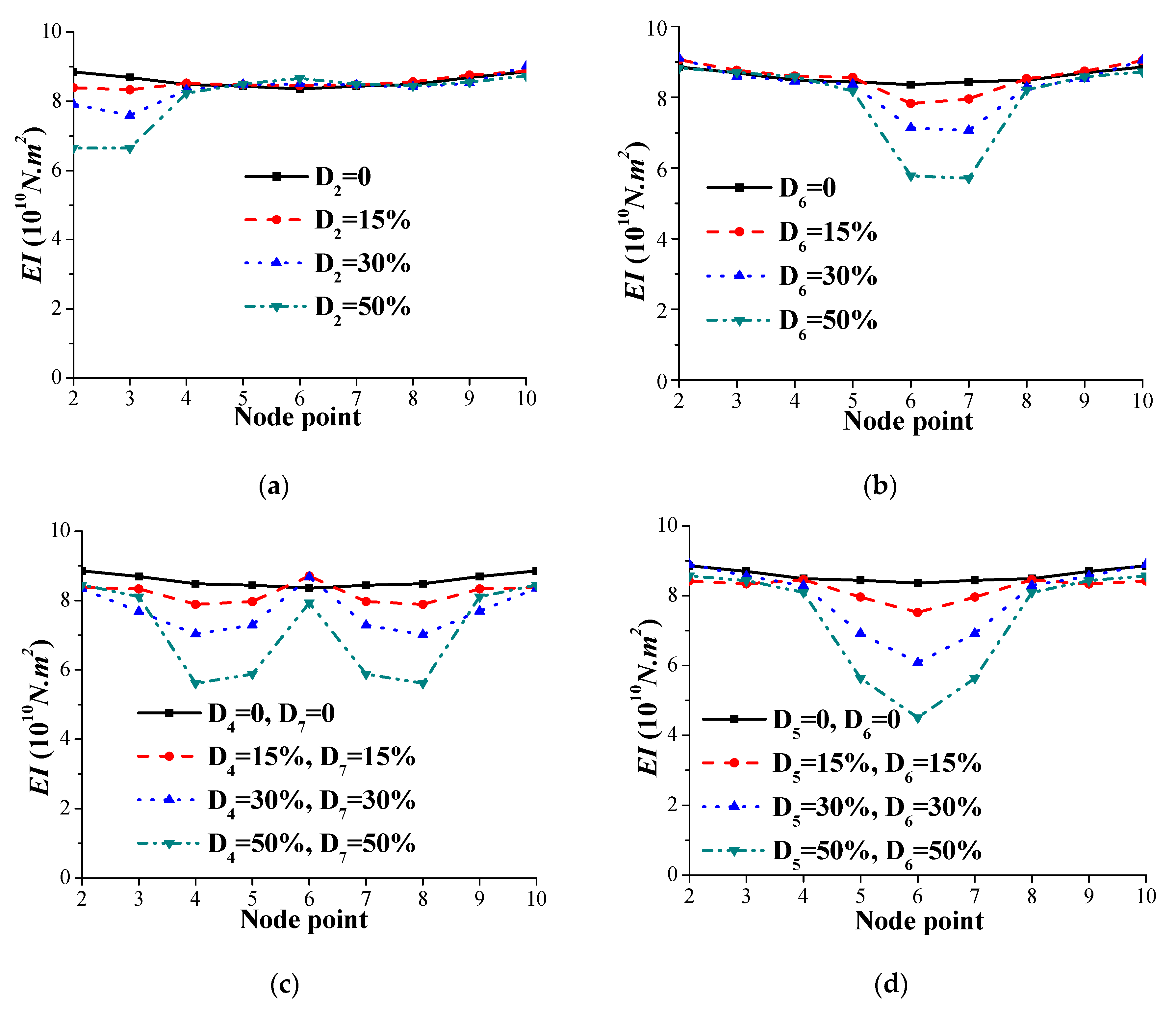
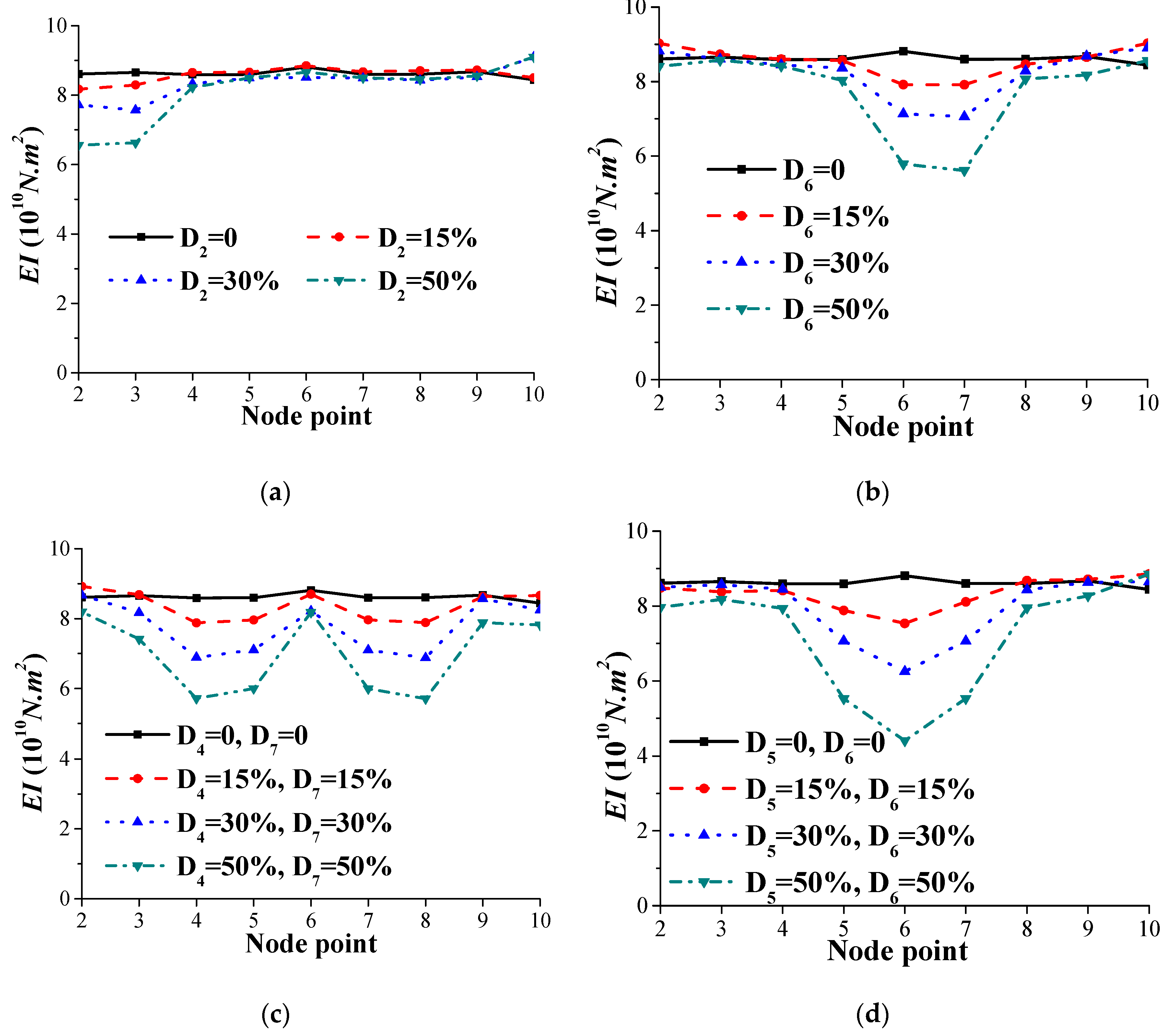
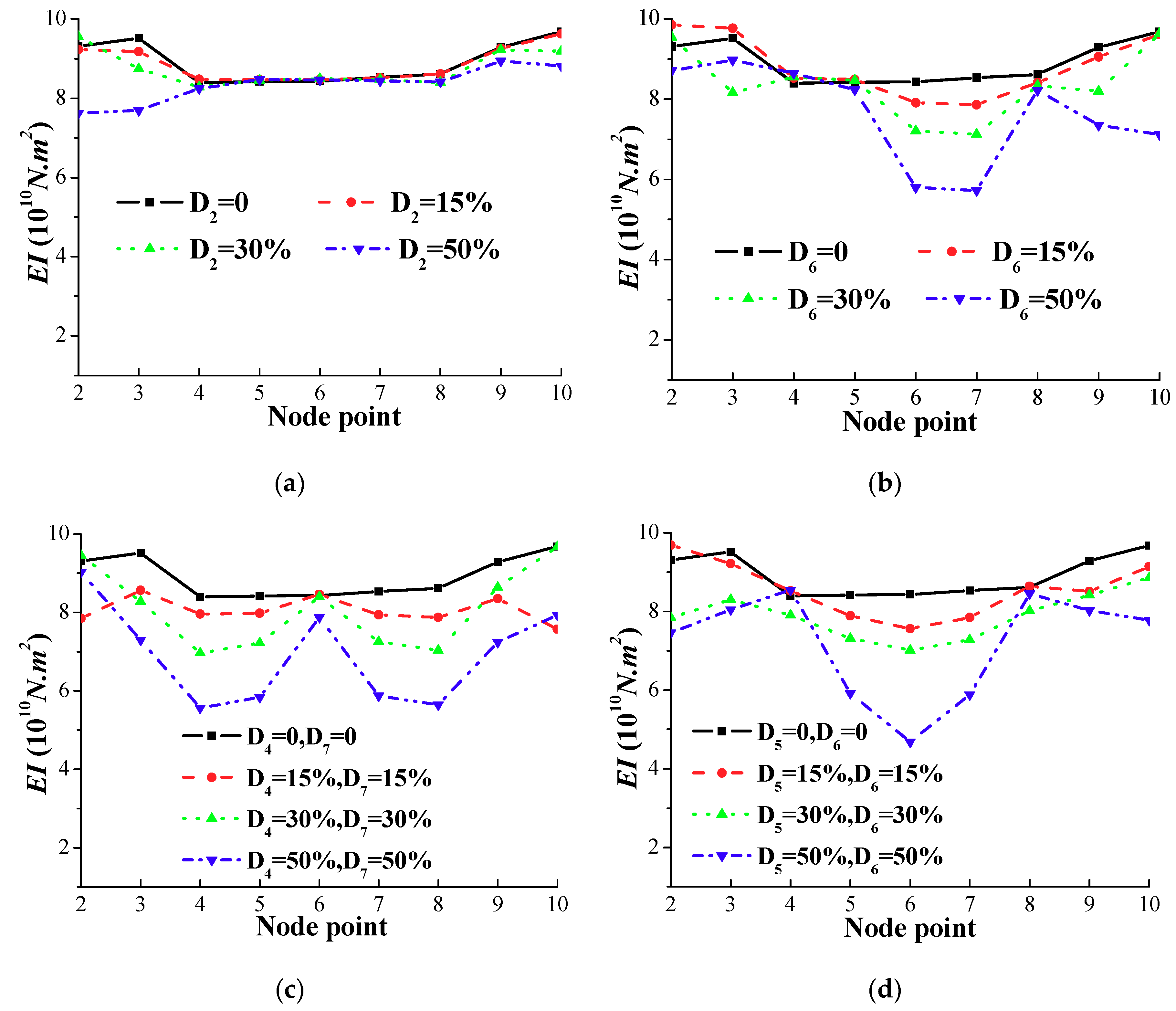
4. Damage Scenarios Studied
4.1. Case 1
4.2. Case 2
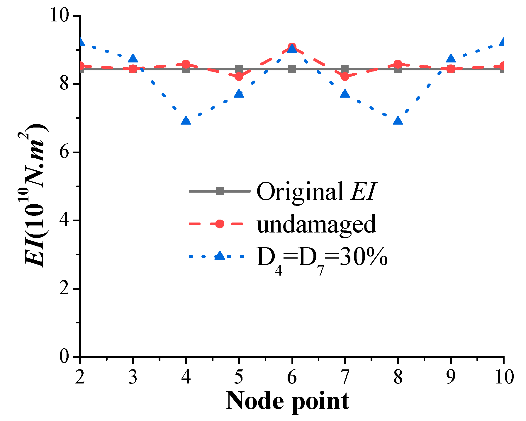
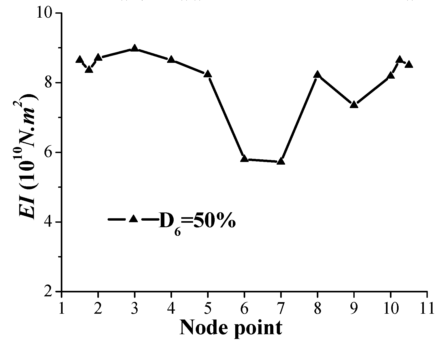
4.3. Case 3
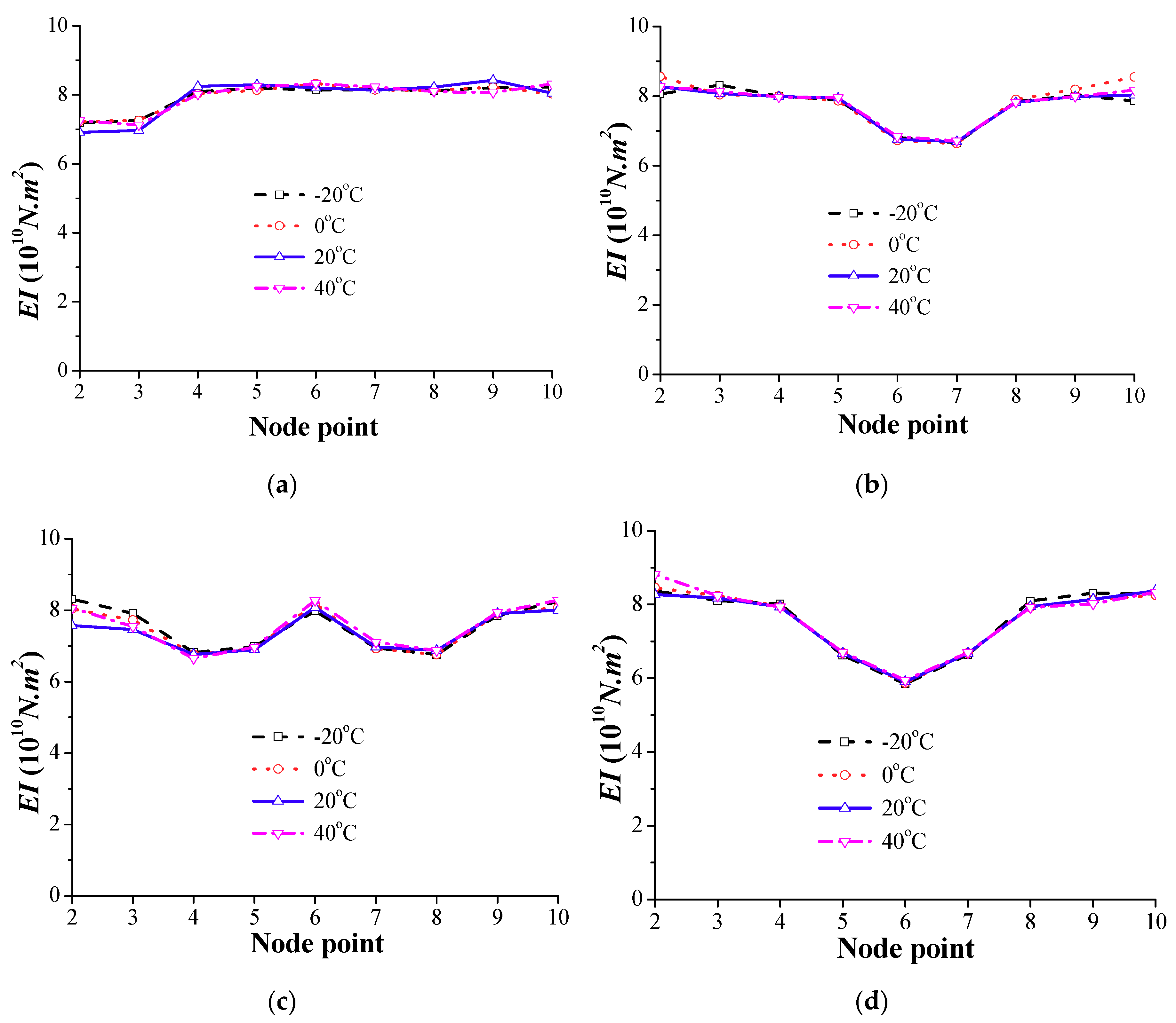
4.4. Case 4
4.5. Discussion on the Boundary Effects
4.6. Discussion on the Variation of Bridge Bearing
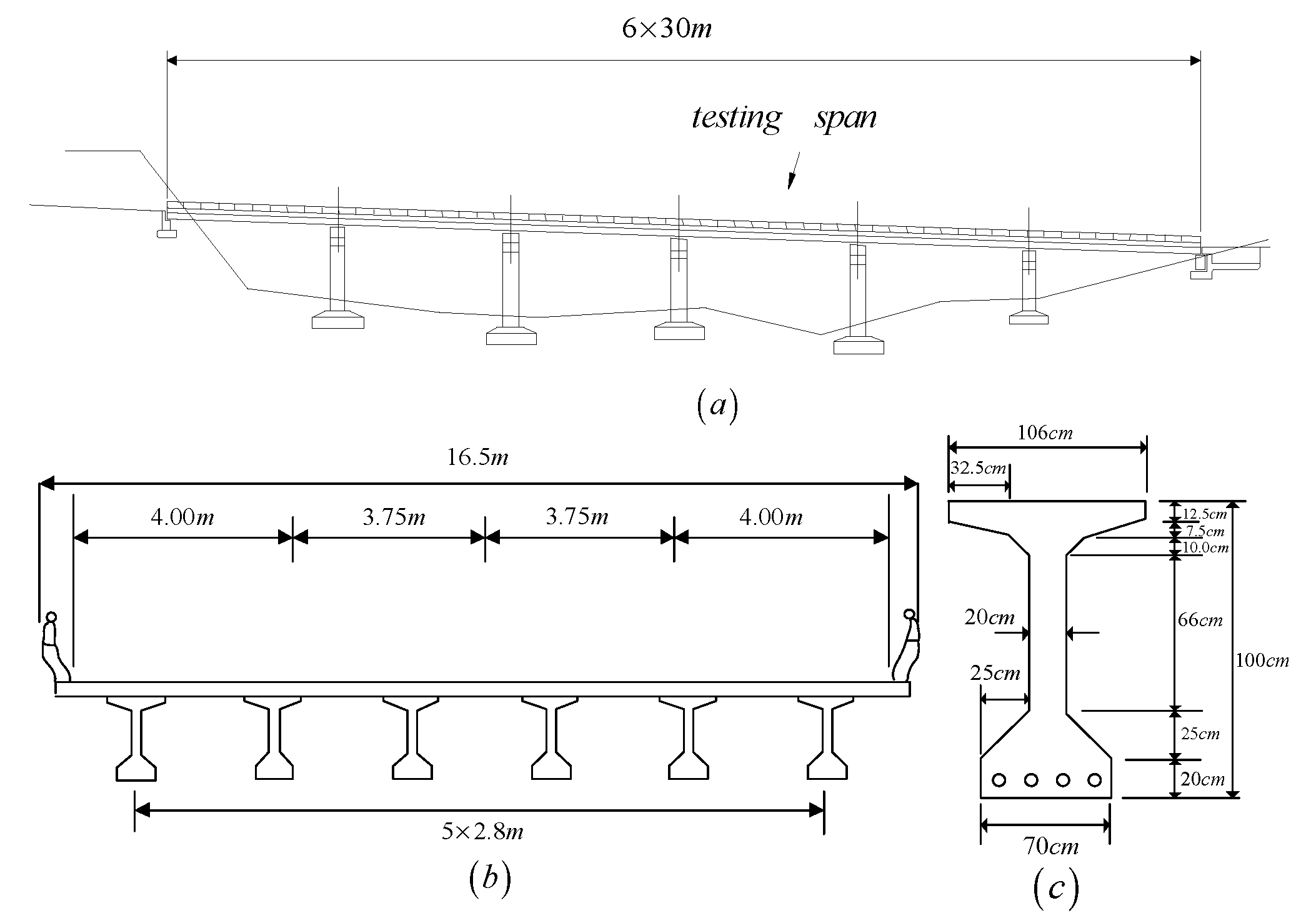
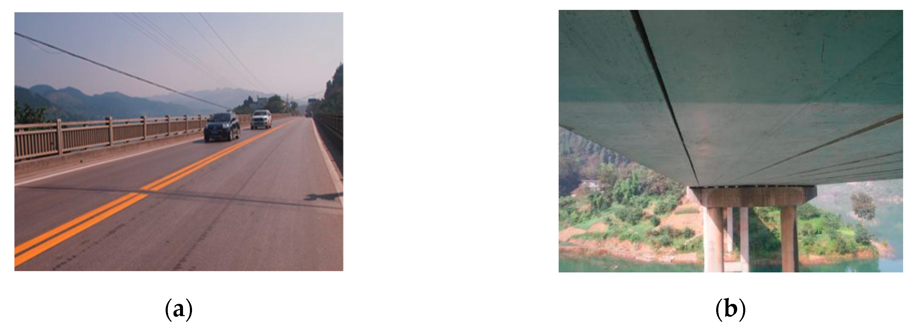
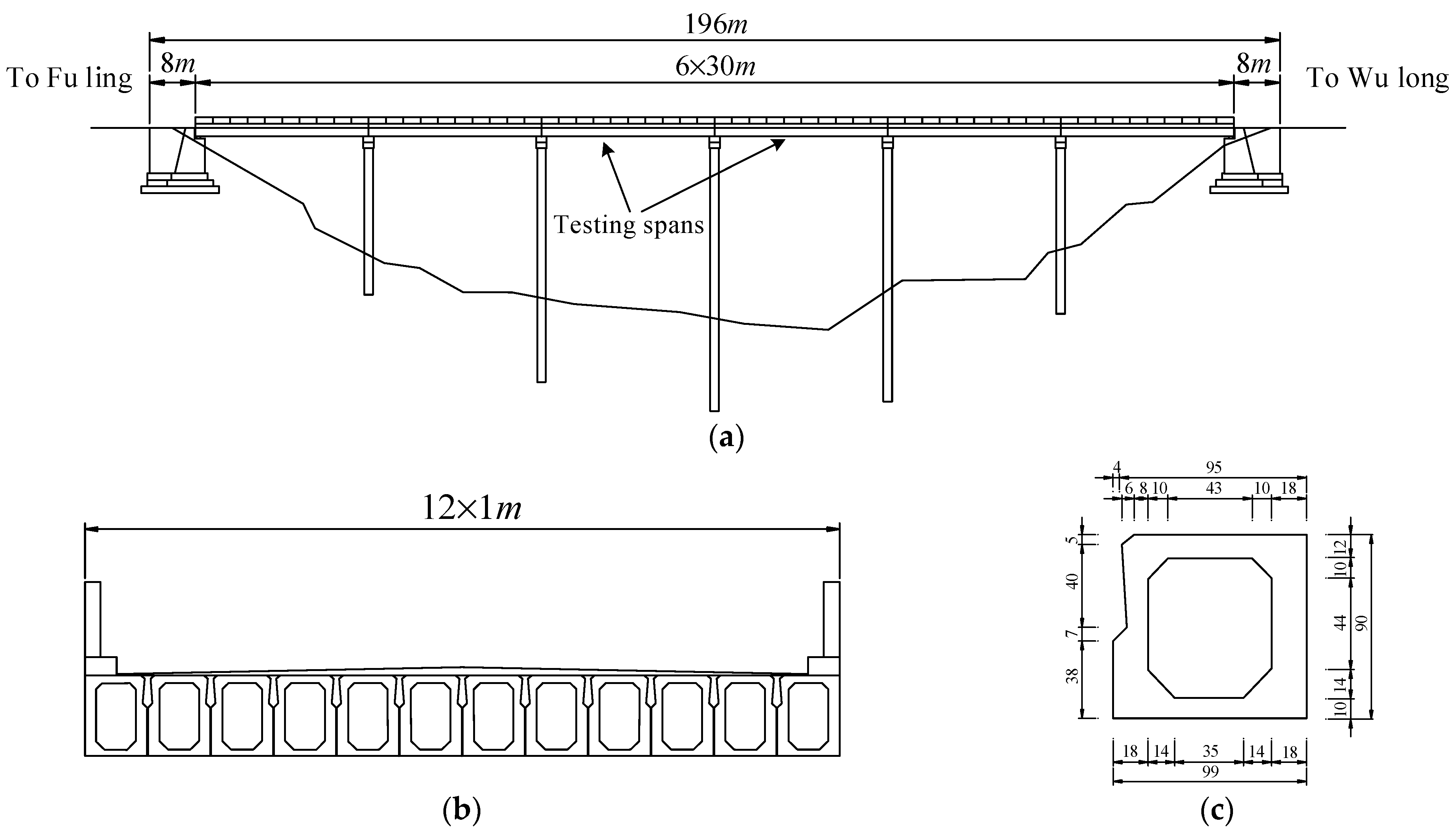
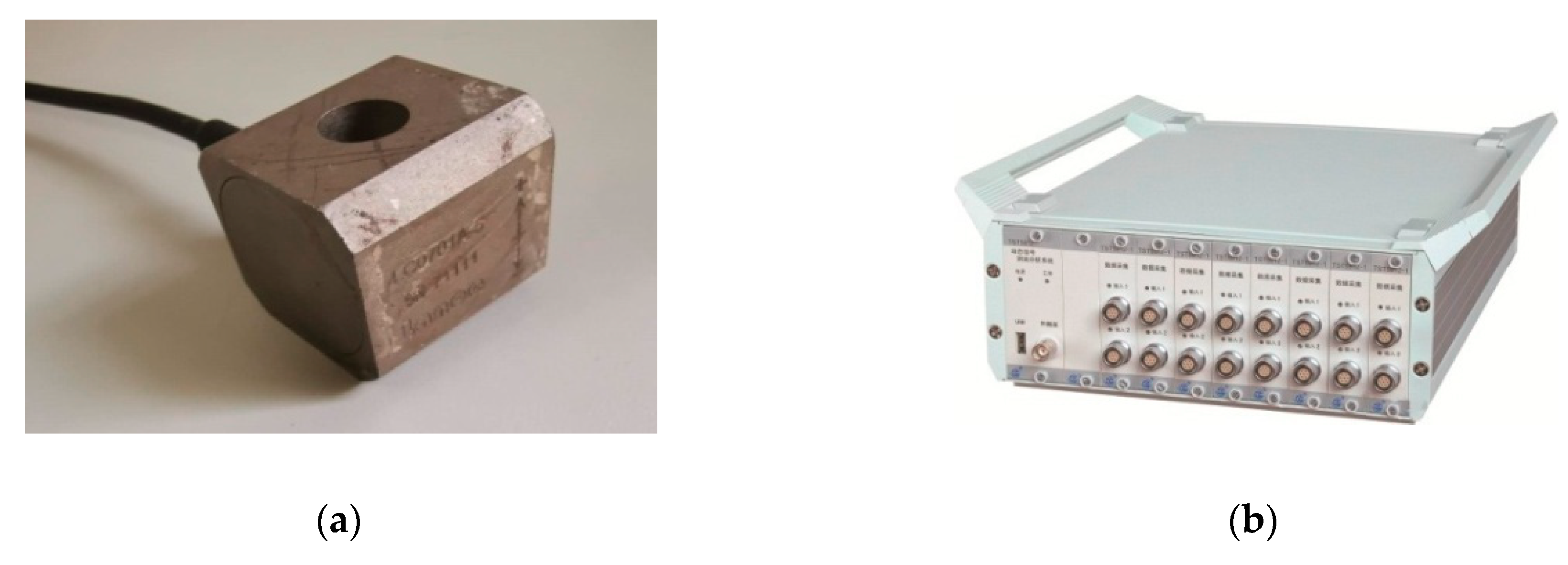
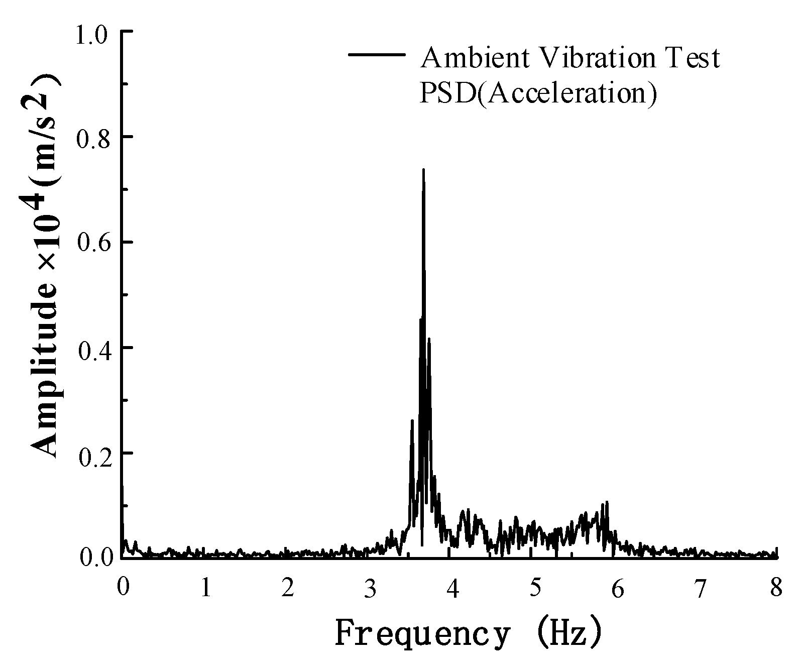
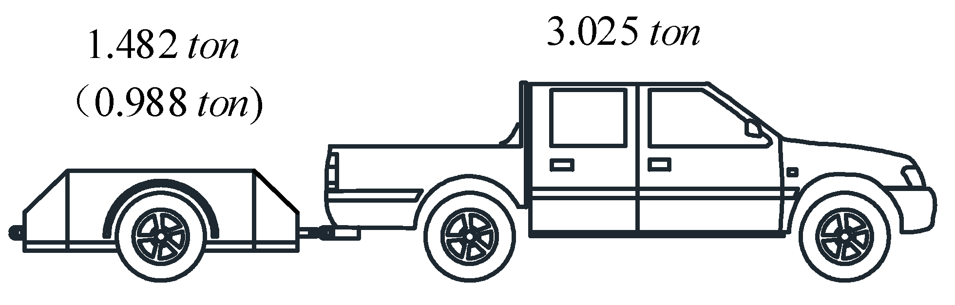
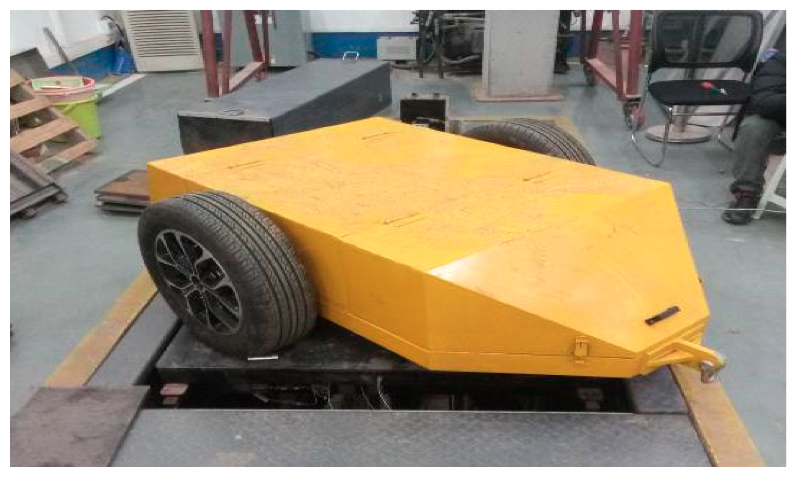
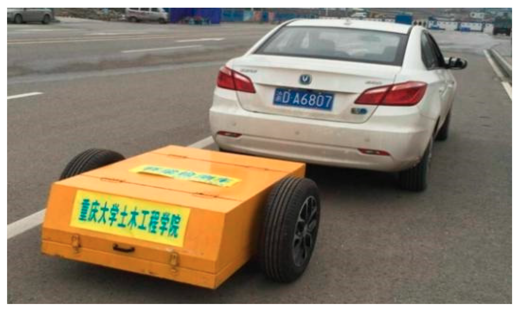
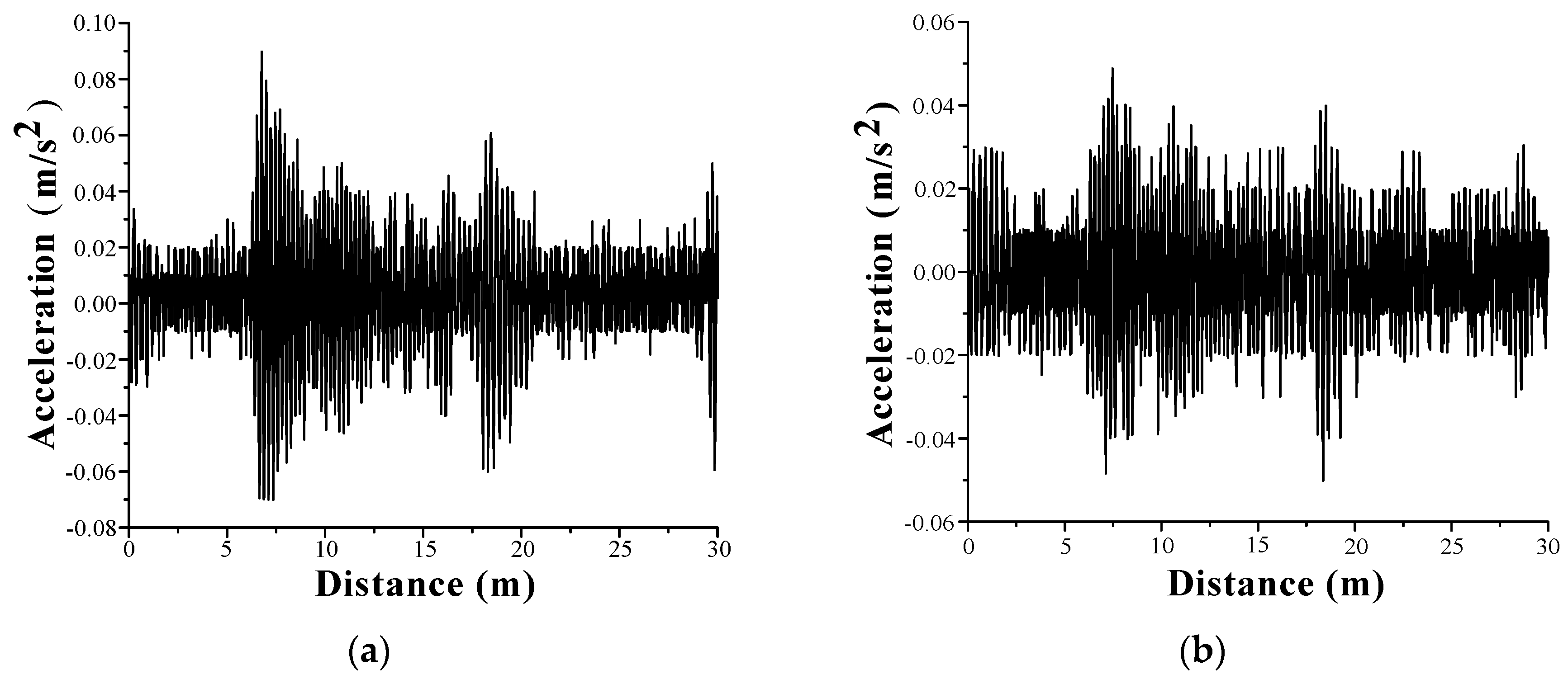
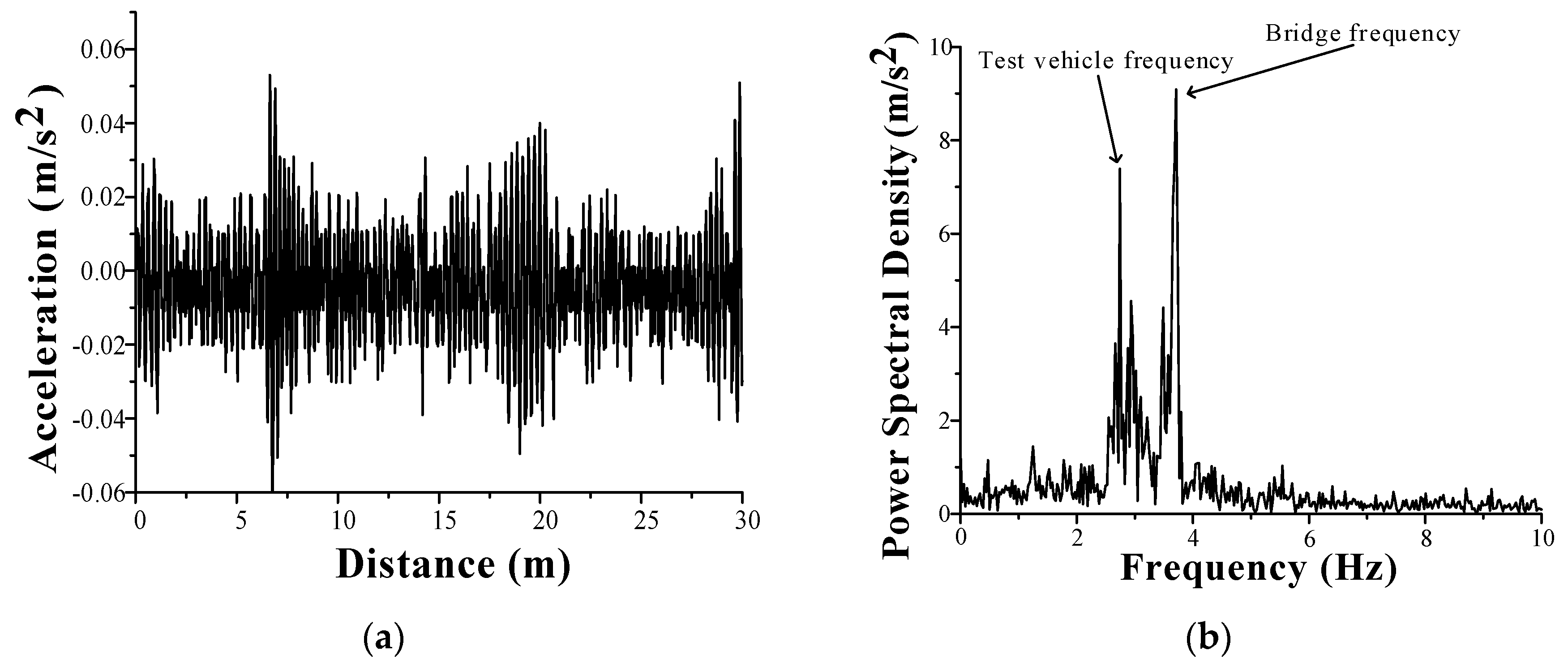
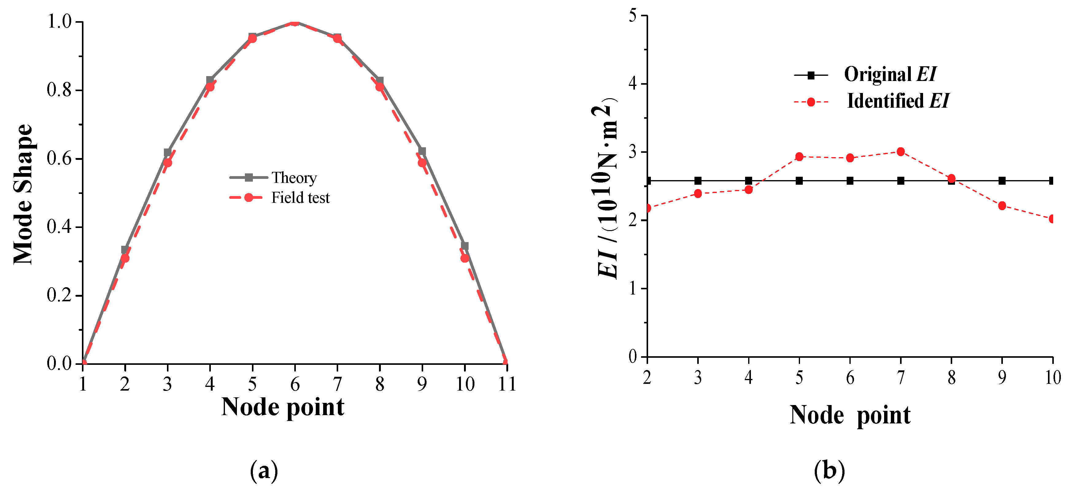
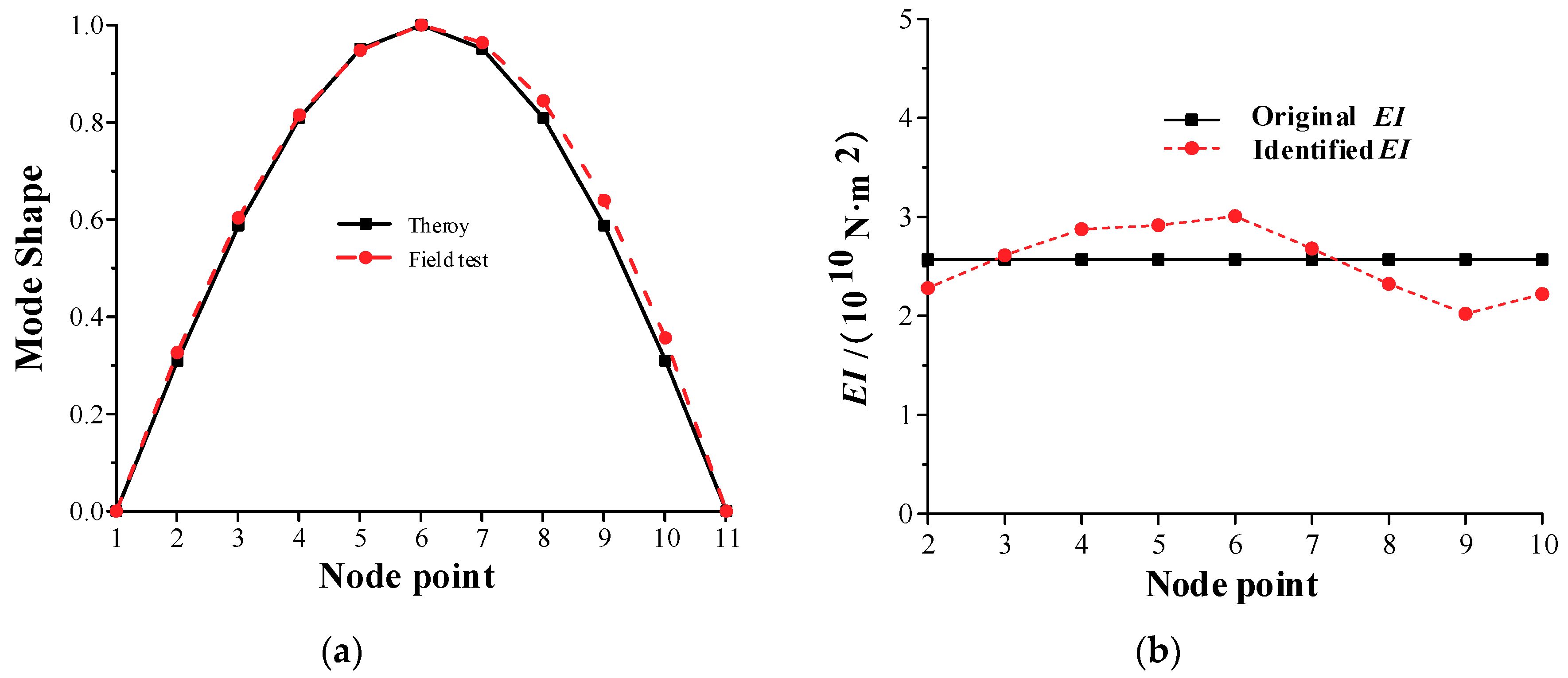
5. Field Test Study
6. Conclusions
- (1)
- Two test vehicles are designed to have identical modal frequency and damping ratio, but the No.2 test vehicle has a mass, stiffness and damping coefficient proportional to those of the No.1 test vehicle. This technique can help to generate a response from an equivalent vehicle of a single vehicle-bridge system that is free from the effect of road surface roughness.
- (2)
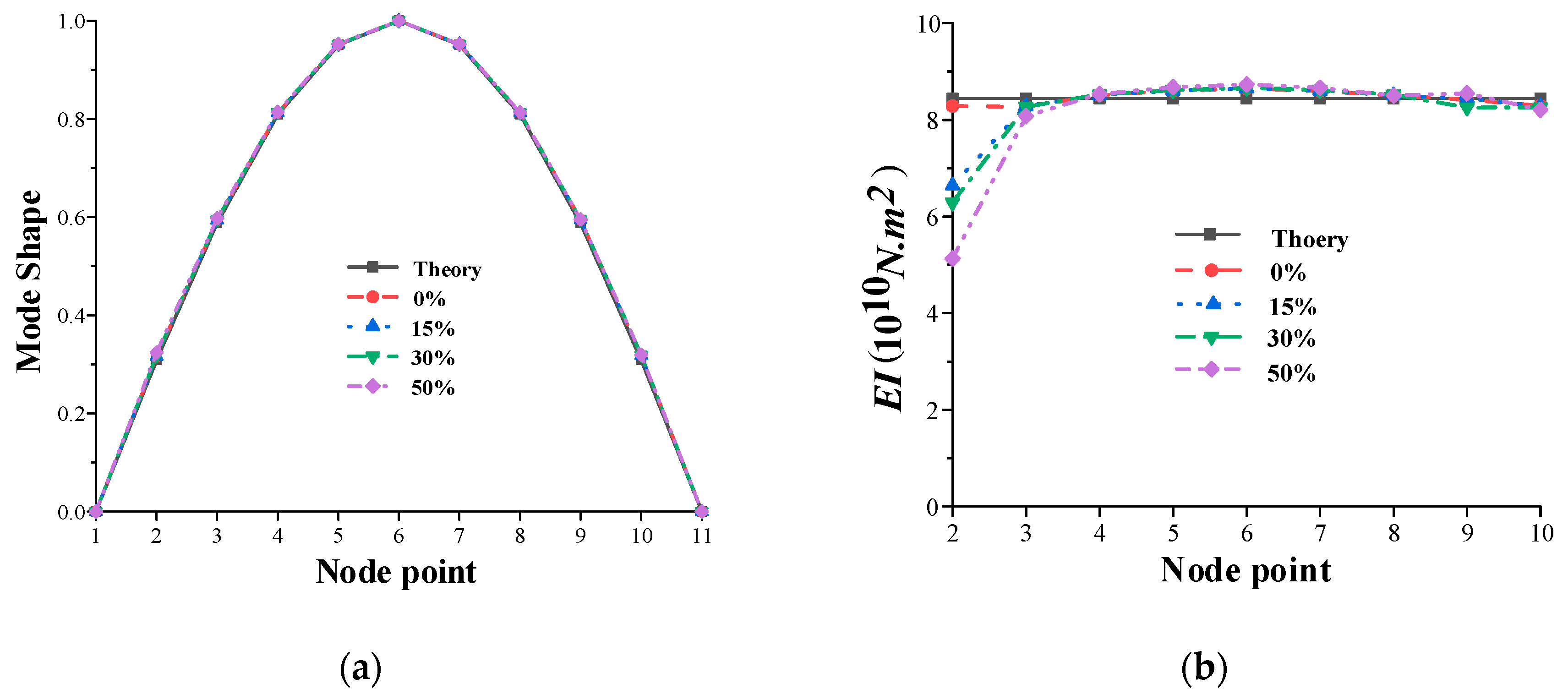
- The first modal frequency and mode shape of the deck structure can be accurately estimated from the response of the equivalent vehicle with consideration of damping of the vehicle-tractor-bridge system, non-uniform test vehicle speed, measurement noise, and different ambient temperatures in the measurements.
- (3)
- The bending stiffness EI of the bridge deck can be better estimated with improvements proposed for the DSC method. For locations such as simply-supported ends of the beam, the improved DSC method can be used to obtain the stiffness by extrapolating the mode shape and using a refined model (or denser data measurements) near these locations.
- (4)
- The tractor-test vehicle technique of non-destructive testing with the proposed modifications has been demonstrated to be feasible for practical application to regular monitoring and evaluation of the structural health condition of a beam-like bridge deck with the advantages of simplicity, mobility, and ease of implementation.
Author Contributions
Funding
Acknowledgments
Conflicts of Interest
References
- Yang, Y.; Mosalam, K.M.; Liu, G.; Wang, X.L. Damage detection using improved direct stiffness calculations-a case study. Int. J. Struct. Stab. Dyn. 2016, 16, 1640002. [Google Scholar] [CrossRef]
- Kim, S.; Oberheim, T.; Pakzad, S.; Fenves, G. Structural Health Monitoring of the Golden Gate Bridge; UC Berkeley Nest Retreat Presentation Jan: Berkeley, CA, USA, 2003; pp. 223–243. [Google Scholar]
- Chan, T.H.; Yu, L.; Tam, H.Y.; Ni, Y.Q.; Liu, S.Y.; Chung, W.H. Fiber Bragg grating sensors for structural health monitoring of Tsing Ma bridge: Background and experimental observation. Eng. Struct. 2006, 28, 648–659. [Google Scholar] [CrossRef]
- Yang, Y.; Yang, L.; Wu, B.; Yao, G.; Li, H.; Robert, S. Safety prediction using vehicle safety evaluation model passing on long-span bridge with fully connected neural network. Adv. Civ. Eng. 2019, 2019, 8130240. [Google Scholar] [CrossRef]
- Yang, Y.B.; Lin, C.W.; Yau, J.D. Extracting bridge frequencies from the dynamic response of a passing vehicle. J. Sound Vib. 2004, 272, 471–493. [Google Scholar] [CrossRef]
- Lin, C.W.; Yang, Y.B. Use of a passing vehicle to scan the fundamental bridge frequencies: An experimental verification. Eng. Struct. 2005, 27, 18651–18878. [Google Scholar] [CrossRef]
- Yang, Y.B.; Chen, W.F.; Yu, H.W.; Chan, C.S. Experimental study of a hand-drawn cart for measuring the bridge frequencies. Eng. Struct. 2013, 57, 2222–2231. [Google Scholar] [CrossRef]
- Yang, Y.B.; Chen, W.F. Extraction of bridge frequencies from a moving test vehicle by stochastic subspace identification. J. Bridge Eng. 2016, 21, 4015053. [Google Scholar] [CrossRef]
- Yang, Y.B.; Li, Y.C.; Chang, K. Constructing the mode shapes of a bridge from a passing vehicle: A theoretical study. Smart Struct. Syst. 2014, 13, 797–819. [Google Scholar] [CrossRef]
- Malekjafarian, A.; Obrien, E.J. On the use of a passing vehicle for the estimation of bridge mode shapes. J. Sound Vib. 2017, 397, 77–91. [Google Scholar] [CrossRef]
- Malekjafarian, A.; Obrien, E.J. Identification of bridge mode shapes using Short Time Frequency Domain Decomposition of the responses measured in a passing vehicle. Eng. Struct. 2014, 81, 386–397. [Google Scholar] [CrossRef]
- Gomeza, H.C.; Fanning, P.J.; Feng, M.Q.; Lee, S. Testing and long-term monitoring of a curved concrete box girder bridge. Eng. Struct. 2011, 33, 2861–2869. [Google Scholar] [CrossRef]
- Kim, J.; Lynch, J.P. Experimental analysis of vehicle–bridge interaction using a wireless monitoring system and a two-stage system identification technique. Mech. Syst. Signal Process. 2012, 28, 31–39. [Google Scholar] [CrossRef]
- Siringoringo, D.M.; Fujino, Y. Estimating bridge fundamental frequency from vibration response of instrumented passing vehicle: Analytical and experimental study. Adv. Struct. Eng. 2012, 15, 417–433. [Google Scholar] [CrossRef]
- Sitton, J.D.; Zeinali, Y.; Story, B.A. Frequency Estimation onTwo-Span Continuous Bridges Using Dynamic Responses of PassingVehicles. J. Eng. Mech. 2020, 146, 4019115. [Google Scholar] [CrossRef]
- Gonzalez, A.; OBrien, E.J.; McGetrick, P.J. Identification of damping in a bridge using a moving instrumented vehicle. J. Sound Vib. 2012, 331, 4115–4131. [Google Scholar] [CrossRef]
- Keenahan, J.; Obrien, E.J.; McGetrick, P.J.; González, A. The use of a dynamic truck-trailer drive-by system to monitor bridge damping. Struct. Health Monit. 2014, 13, 143–157. [Google Scholar] [CrossRef]
- Yang, Y.B.; Zhang, B.; Chen, Y.N.; Qian, Y.; Wu, Y.T. Bridge damping identification by vehicle scanning method. Eng. Struct. 2019, 183, 637–645. [Google Scholar] [CrossRef]
- Chang, K.C.; Wu, F.B.; Yang, Y.B. Effect of road roughness on indirect approach for measuring bridge frequencies form a passing vehicle. Interact. Multiscale Mech. 2010, 3, 299–308. [Google Scholar] [CrossRef]
- Yang, Y.B.; Li, Y.C.; Chang, K.C. Using two connected vehicles to measure the frequencies of bridges with rough surface: A theoretical study. Acta Mech. 2012, 223, 1851–1861. [Google Scholar] [CrossRef]
- Kong, X.; Cai, C.S.; Kong, B. Numerically Extracting Bridge Modal Properties from Dynamic Responses of Moving Vehicles. J. Eng. Mech. 2016, 142, 4016025. [Google Scholar] [CrossRef]
- Bu, J.Q.; Law, S.S.; Zhu, X.Q. Innovative bridge condition assessment from dynamic response of a passing vehicle. J. Eng. Mech. 2006, 132, 1372–1379. [Google Scholar] [CrossRef]
- Kim, C.W.; Kawatani, M. Pseudo-static approach for damage identification of bridges based on coupling vibration with a moving vehicle. Struct. Infrastruct. Eng. 2008, 4, 371–379. [Google Scholar] [CrossRef]
- Yin, S.S.; Tang, C.Y. Identifying cable tension loss and deck damage in a cable-stayed bridge using a moving vehicle. J. Vib. Acoust. 2011, 133, 898–923. [Google Scholar] [CrossRef]
- Lu, Z.R.; Liu, J.K. Identification of both structural damages in bridge deck and vehicle parameters using measured dynamic response. Comput. Struct. 2011, 89, 1397–1405. [Google Scholar] [CrossRef]
- Miyamoto, A.; Yabe, A. Bridge condition assessment based on vibration response of passenger vehicle. J. Phys. 2011, 305, 1–10. [Google Scholar] [CrossRef]
- Zhang, Y.; Lie, S.T.; Xiang, Z.H. Damage detection method based on operating deflection shape curvature extracted from dynamic response of a passing vehicle. Mech. Syst. Signal Process. 2013, 35, 238–254. [Google Scholar] [CrossRef]
- Zhang, Y.; Wang, L.Q.; Xiang, Z.H. Damage detection by mode shape squares extracted from a passing vehicle. J. Sound Vib. 2012, 331, 291–307. [Google Scholar] [CrossRef]
- Li, Z.; Au, F.T.K. Damage detection of bridges using response of vehicle considering road surface roughness. Int. J. Struct. Stab. Dyn. 2015, 15, 1450057. [Google Scholar] [CrossRef]
- Feng, D.M.; Feng, M.Q. Output-only damage detection using vehicle-induced displacement response and mode shape curvature index. Struct. Control. Health Monit. 2016, 23, 1088–1107. [Google Scholar] [CrossRef]
- Mei, Q.; Gul, M.; Boay, M. Indirect health monitoring ofbridges using Mel-frequency cepstral coefficients and principal componentanalysis. Mech. Syst. Signal Process. 2019, 119, 523–546. [Google Scholar] [CrossRef]
- Yang, Y.; Zhu, Y.H.; Wang, L.L.; Jia, B.Y.L.; Jin, R.Y. Structural Damage identification of bridges from passing test vehicles. Sensors 2018, 18, 4035. [Google Scholar] [CrossRef] [PubMed]
- Shi, Z.Y.; Law, S.S.; Zhang, L.M. Improved damage quantification from elemental modal strain energy change. J. Eng. Mech. 2002, 128, 521–529. [Google Scholar] [CrossRef]
- Kim, B.S.; Yoo, S.H.; Yeo, G.H. Characterization of crack detection on gusset plates using strain mode shapes. In Proceedings of the 23rd International Modal Analysis Conference (IMAC XXIII), Orlando, FL, USA, 31 January 31–3 February 2005. [Google Scholar]
- Li, J.; Law, S.S.; Ding, Y. Substructure damage identification based on response reconstruction in frequency domain and model updating. Eng. Struct. 2012, 41, 270–284. [Google Scholar] [CrossRef]
- Zhong, H.; Yang, M.J. Damage detection for plate-like structures using generalized curvature mode shape method. J. Civ. Struct. Health Monit. 2016, 6, 141–152. [Google Scholar] [CrossRef]
- Samami, H.; Oyadiji, S.O. Simulation and detection of small crack-like surface flaws and slots in simply-supported beams using curvature analysis of analytical and numerical modal displacement data. Eng. Comput. 2016, 33, 1969–2006. [Google Scholar] [CrossRef]
- Yang, Y.; Li, J.L.; Zhou, C.H.; Law, S.S.; Lv, L. Damage detection of structures with parametric uncertainties based on fusion of statistical moments. J. Sound Vib. 2019, 442, 200–219. [Google Scholar] [CrossRef]
- OBrien, E.J.; McGetrick, P.J.; Gonzalez, A. A drive-by inspection system via vehicle moving force identification. Smart Struct. Syst. 2014, 13, 821–848. [Google Scholar] [CrossRef]
- Dao, P.B.; Staszewski, W.J.; Klepka, A. Stationarity-based approach for the selection of lag length in cointegration analysis used for structural damage detection. Comput. Aided Civ. Infrastruct. Eng. 2017, 32, 138–153. [Google Scholar] [CrossRef]
- Niemann, H.; Morlier, J.; Shahdin, A.; Gourinat, Y. Damage localization using experimental modal parameters and topology optimization. Mech. Syst. Signal Process. 2010, 24, 636–652. [Google Scholar] [CrossRef]
- Li, W.M.; Jiang, Z.H.; Wang, T.L.; Zhu, H.P. Optimization method based on generalized pattern search algorithm to identify bridge parameters indirectly by a passing vehicle. J. Sound Vib. 2014, 333, 364–380. [Google Scholar] [CrossRef]
- Maeck, J. Damage Assessment of Civil Engineering Structure by Vibration Moanitoring. Ph.D. Thesis, Department of Civil Engineering, KatholiekeUniversiteit Leuven, Brussels, Belgium, 2003. [Google Scholar]
- Huth, O.; Feltrin, G.; Maeck, J.; Kilic, N.; Motavalli, M. Damage identification using modal data: Experiences on a prestressed concrete bridge. J. Struct. Eng. 2005, 131, 1898–1910. [Google Scholar] [CrossRef]
- Yang, Y.; Liu, H.; Mosalam, K.M.; Huang, S.N. An improved direct stiffness calculation method for damage detection of beam structures. Struct. Control Health Monit. 2013, 20, 835–851. [Google Scholar] [CrossRef]
- Wang, L.H. Studies on Non-Destructive Damage Detection of Bridges Based on Linear and Nonlinear Dynamic Characteristics. Ph.D. Thesis, College of Architecture, Civil Engineering, Beijing University of Technology, Beijing, China, 2006. [Google Scholar]
- Yang, Y.; Yang, Y.B.; Chen, Z.X. Seismic damage assessment of RC structures under shaking table tests using the modified direct stiffness calculation method. Eng. Struct. 2017, 131, 545–586. [Google Scholar] [CrossRef]
- Yau, J.D.; Yang, Y.B.; Kuo, S.R. Impact response of high-speed rail bridges and riding comfort of rail car. Eng. Struct. 1999, 21, 836–844. [Google Scholar] [CrossRef]
- Yau, J.D.; Yang, J.P.; Yang, Y.B. Wavenumber-based technique for detecting slope discontinuity in simple beams using moving test vehicle. Int. J. Struct. Stab. Dyn. 2017, 17, 1750060. [Google Scholar] [CrossRef]
- ISO 8608. Mechanical Vibration-Road Surface Profiles—Reporting of Measured Data; ISO: Geneva, Switzerland, 1995. [Google Scholar]
- Gu, J.F.; Gul, M.; Wu, X.G. Damage detection under varying temperature using artificial neutral networks. Struct. Control Health Monit. 2017, 24, 1998. [Google Scholar] [CrossRef]
- Hios, J.D.; Fassois, S.D. A global statistical model based approach for vibration response-only damage detection under various temperatures: A proof-of-concept study. J. Mech. Syst. Signal Process. 2014, 49, 77–94. [Google Scholar] [CrossRef]
- Deng, L.; Duan, L.L.; He, W. Study on vehicle model for vehicle-bridge coupling vibration of highway bridge in China. China J. Highw. Transp. 2018, 31, 92–100. [Google Scholar]


| Properties of Test Vehicle | No.1 | No.2 |
|---|---|---|
| Frequency (Hz) | 0.503 | 0.503 |
| Mass (kg) | 5000 | 10,000 |
| Stiffness (kN/m) | 50 | 100 |
| Damping coefficient | 1 | 2 |
| Speed (m/s) | 1 | 1 |
| Properties of the No.1 Test Vehicle | No.1-1 | No.1-2 | No.1-3 | No.1-4 | No.1-5 | No.1-6 |
|---|---|---|---|---|---|---|
| Frequency (Hz) | 0.503 | 0.650 | 1.125 | 1.592 | 2.251 | 2.757 |
| Mass (Kg) | 5000 | 3000 | 1000 | 500 | 1000 | 1000 |
| (kN/m) | 50 | 50 | 50 | 50 | 200 | 300 |
| Damping coefficient () | 1 | 1 | 1 | 1 | 1 | 1 |
| Speed (m/s) | 1 | 1 | 1 | 1 | 1 | 1 |
| Cases | Vehicle | Bridge | Road Surface Roughness | Temperature (°C) |
|---|---|---|---|---|
| 1 | damped | undamped | -- | - |
| 2 | damped | damped | -- | - |
| 3 | damped | damped | Class C, D | - |
| 4 | damped | damped | Class C | −20, 0, 20 & 40 |
| Damage Scenario | Damage Element(s) | Related Node Numbers | Reduction in Element Stiffness (%) | |||
|---|---|---|---|---|---|---|
| (a) | (b) | (c) | (d) | |||
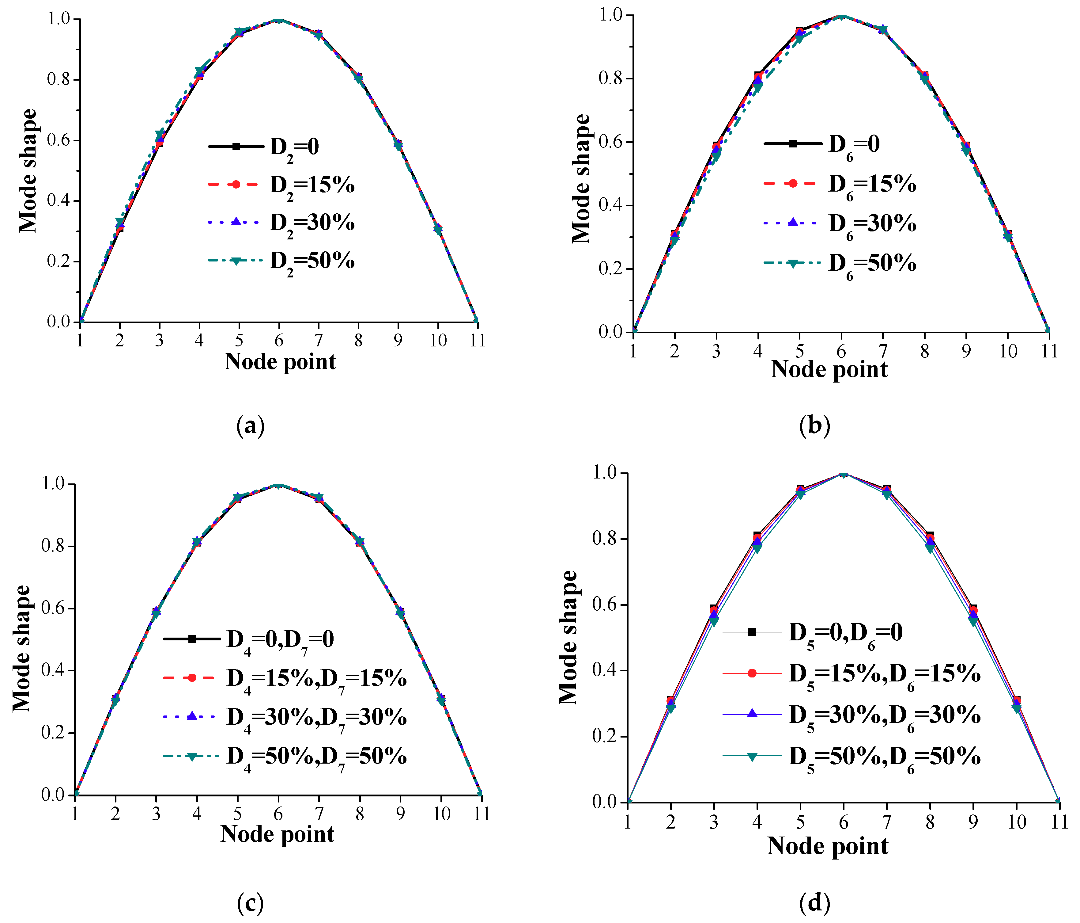
| A | D2 | 2, 3 | D2 = 0 | D2 = 15 | D2 = 30 | D2 = 50 |
| B | D6 | 6, 7 | D6 = 0 | D6 = 15 | D6 = 30 | D6 = 50 |
| C | D4, D7 | 4, 5 &7, 8 | D4 = 0 D7 = 0 | D4 = 15 D7 = 15 | D4 = 30 D7 = 30 | D4 = 50 D7 = 50 |
| D | D5, D6 | 5, 6, 7 | D5 = 0 D6 = 0 | D5 = 15 D6 = 15 | D5 = 30 D6 = 30 | D5 = 50 D6 = 50 |
© 2020 by the authors. Licensee MDPI, Basel, Switzerland. This article is an open access article distributed under the terms and conditions of the Creative Commons Attribution (CC BY) license (http://creativecommons.org/licenses/by/4.0/).
Share and Cite
Yang, Y.; Cheng, Q.; Zhu, Y.; Wang, L.; Jin, R. Feasibility Study of Tractor-Test Vehicle Technique for Practical Structural Condition Assessment of Beam-Like Bridge Deck. Remote Sens. 2020, 12, 114. https://doi.org/10.3390/rs12010114
Yang Y, Cheng Q, Zhu Y, Wang L, Jin R. Feasibility Study of Tractor-Test Vehicle Technique for Practical Structural Condition Assessment of Beam-Like Bridge Deck. Remote Sensing. 2020; 12(1):114. https://doi.org/10.3390/rs12010114
Chicago/Turabian StyleYang, Yang, Quan Cheng, Yuanhao Zhu, Lilei Wang, and Ruoyu Jin. 2020. "Feasibility Study of Tractor-Test Vehicle Technique for Practical Structural Condition Assessment of Beam-Like Bridge Deck" Remote Sensing 12, no. 1: 114. https://doi.org/10.3390/rs12010114
APA StyleYang, Y., Cheng, Q., Zhu, Y., Wang, L., & Jin, R. (2020). Feasibility Study of Tractor-Test Vehicle Technique for Practical Structural Condition Assessment of Beam-Like Bridge Deck. Remote Sensing, 12(1), 114. https://doi.org/10.3390/rs12010114