1. Introduction
The innovative Global Navigation Satellite System Reflectometry (GNSS-R) technique, offering exploitation of existing GNSS signals reflected off the Earth’s surface, has significantly grown in interest as an Earth observation technology to retrieve a variety of geophysical parameters [
1,
2]. Ocean surface wind monitoring using GNSS-R measurements, as a bistatic radar forward scatterometer, is one of the latest promising applications. TechDemoSat-1 (TDS-1), launched in 2014, fully demonstrated the capabilities of GNSS-R in retrieving the state of the ocean, and consequently, in obtaining high-quality winds [
3]. The Cyclone Global Navigation Satellite System (CYGNSS) was launched in December 2016 and provides wind data with an unprecedented sampling rate. CYGNSS consists of eight microsatellites in the inclined orbits [
4,
5]. In addition, further ideas and upcoming GNSS-R missions are being developed [
6,
7,
8].
GNSS-R satellite missions can provide a sufficient observation frequency for ocean surface monitoring, exploiting the high and growing number of GNSS transmitters and the easily employable low-cost, low-mass, and low-power GNSS receivers. In addition, it is known that GNSS L-band signals are affected by a much lower level of attenuation and scattering by clouds or raindrops in the atmosphere, compared to those from the conventional Ku- and C-band scatterometers. The general reliability of wind speed products during rainfalls is documented [
9]. These advantages can be potentially a solution to overcome the limitations in capturing and forecasting severe weather events. Weather models performance degrade during extreme events due to the lack of high spatiotemporal-resolution data and the obscurity of traditional remote sensing instruments during severe weathers. Consequently, improving severe weather forecasting is the overall objective of CYGNSS and the mission studies tropical cyclone inner core process.
Rain can affect ocean monitoring with scatterometers in two ways. First, raindrops impinging the ocean surface alter the wind-induced radar signature, which, in case of GNSS-R scatterometry, is the quasi-specular reflections from multiple facets. They can create rings, stalks, and crowns [
10] which alter the surface roughness, and consequently, the wind retrieval quality. Rain splash effect on GNSS-R observations is discussed [
11] and a decrease in Bistatic Radar Cross Section (BRCS) at low wind speeds (≈<5 m/s) is demonstrated both with TDS-1 data analysis and based on model simulations. At high enough winds (≈>5 m/s), the intensity of forward quasi-specular scattering is controlled by surface gravity waves with lengths larger than several wavelengths of the reflected signal. As a result, the scatterometric GNSS-R measurements are insensitive to the surface modifications by raindrops impinging on the ocean at high winds.
As the second effect, rain attenuates signals passing through the atmosphere, the phenomenon which this study is focused on. Existing raindrops and water vapor in the atmosphere cause attenuation in Electromagnetic (EM) waves due to the absorption and scattering [
12]. Absorption is explained by the intersection of rain cells and propagation path of EM waves and the absorbed energy is transferred into heat. Deeper absorption happens when the rain cells fill a major part of the Fresnel’s ellipsoid along the signal path. In case of large enough signal frequency, such as 12 to 18 GHz (Ku-band), as the precipitation rate increases, the signal received less at the receiver is scattered from the ocean surface and the majority of the radiation is scattered by the rain layer. These effects significantly degrade the performance of scatterometers operating at Ku-band frequencies [
13].
Although the rain attenuation can cause small-scale effects on GNSS signals, the impact on the diverse applications can be different in size. A small change in the observable cannot be always interpreted as an insignificant bias in the final products but it depends on how the product responses to the observable change. The dependency of the wind speed to a GNSS-R observable is translated by a Geophysical Model Function (GMF) which is a forward operator mapping the observable to the product. Mathematically, assuming that the wind speed GMF is a linear function, we can consider the simplified wind speed retrieval problem as:
where
is a
GMF matrix and
and
are the
n- and
m-dimensional observable and wind speed vectors, respectively. In the case of perturbations, we have
, form which we can estimate the relative error in the wind speed as:
which shows that the final error in the wind speed is a function of condition number
which reads:
Finally, a small change in the observable can cause large biases in the output for problems with a large condition number, so-called ill-conditioned problems.
Normally, in GNSS-R wind speed retrievals, the GMF is a nonlinear function. The condition number for nonlinear functions, unlike the discussed linear problem, is not a constant value, and varies with the point over the domain of the function. The condition number of a nonlinear but differentiable function
f at point
x is
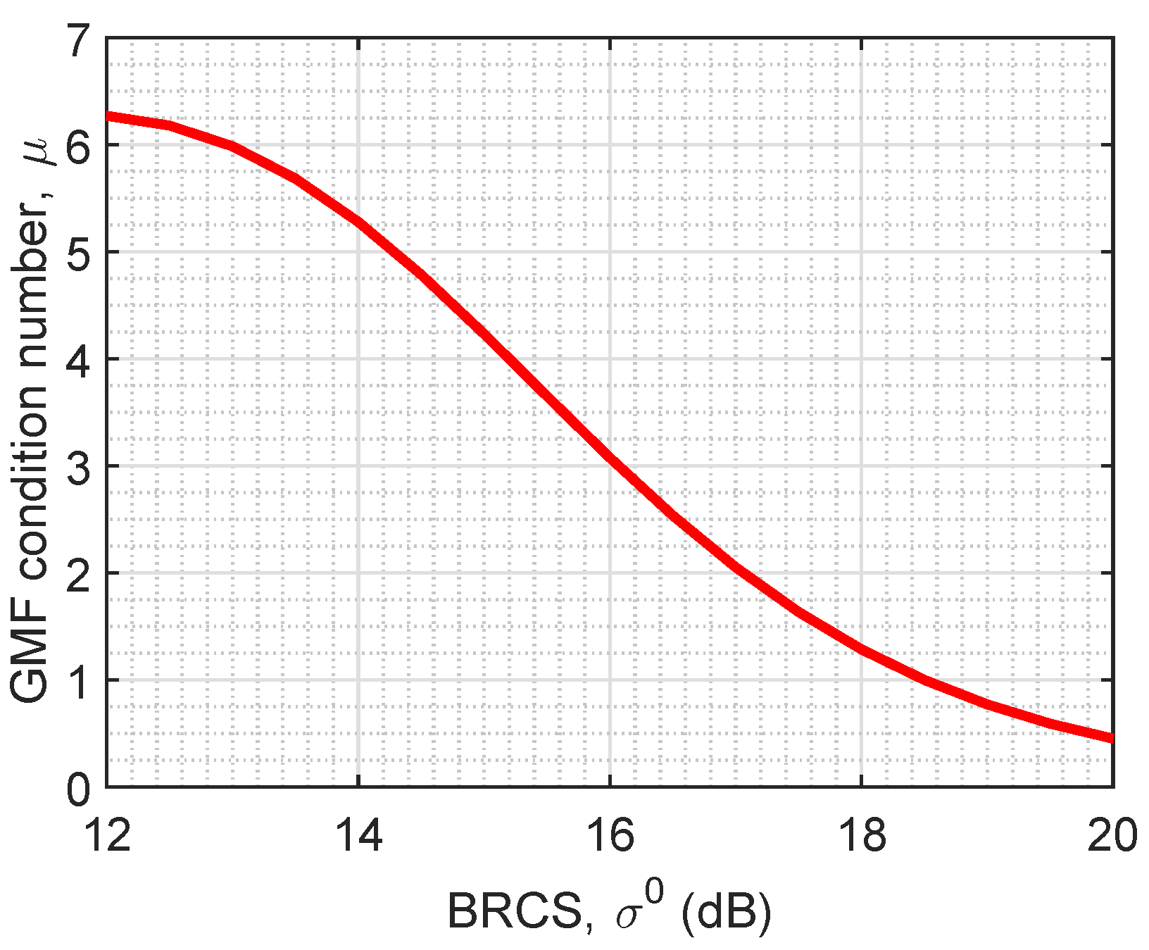
. Hence, a TDS-1 wind speed
GMF, taking the Bistatic Radar Cross Section (BRCS)
as the input argument,
[
9], can be considered and the associated condition number is shown in
Figure 1. Accordingly, at lower values of
, corresponding to higher wind speeds, the condition number is at higher levels. So, at a small enough
, that is at high enough wind speeds, the GMF tends to an ill-conditioned function.
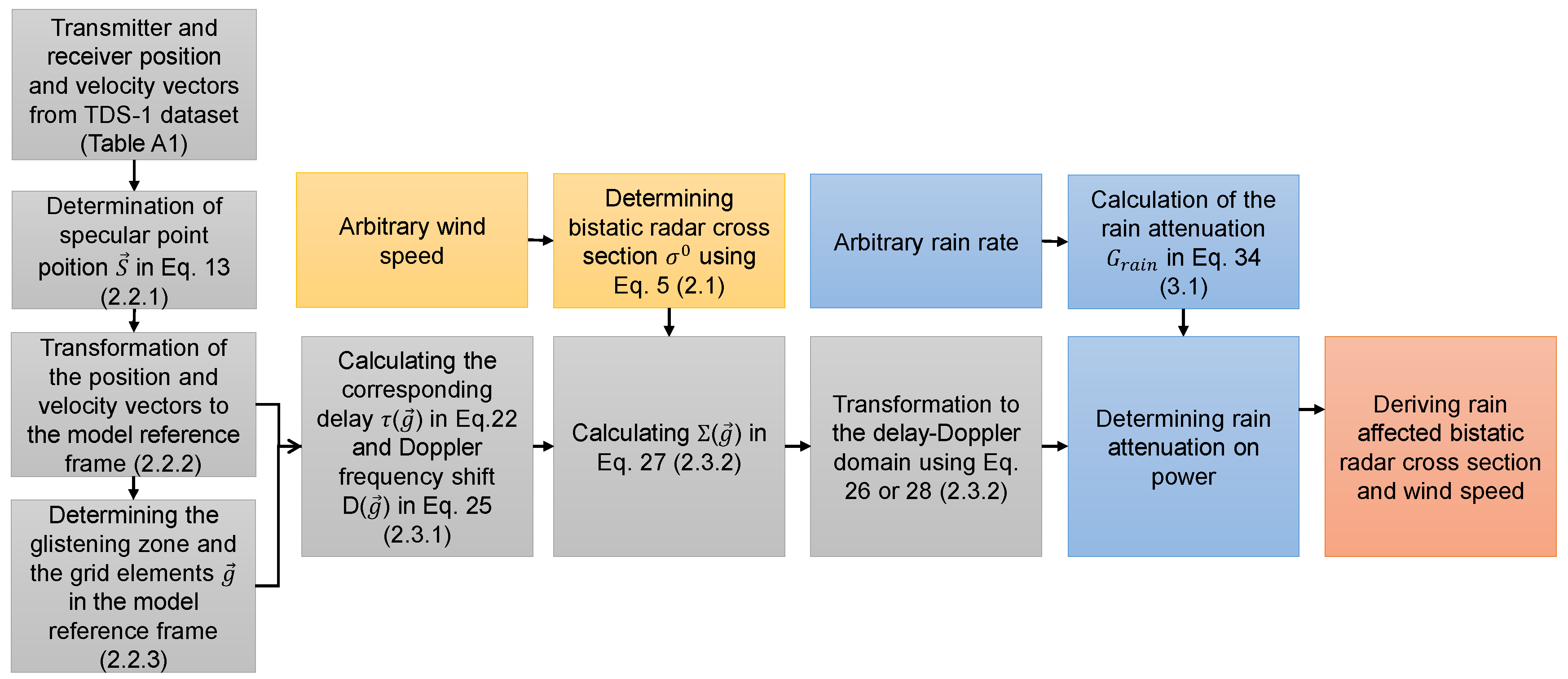
According to the above arguments, small changes in the GNSS-R observables might cause a considerable bias in the wind speed at high-value regions, which signifies the need to a characterization investigation, considering the main objective of CYGNSS. However, conducting data analysis at extreme winds and rains is impossible due to the lack of a sufficient number of observation from extreme events. This study characterizes the effect simulating the delay-Doppler Maps (DDM) and
, as described in
Section 2. Counting rain attenuation effects is explained in
Section 3, which also reports the numerical results. Finally,
Section 4 discusses the outcomes and provides the concluding remarks.
2. Simulating DDMs
In this study, the simulations are based on the bistatic radar equation which reads [
14]:
where
and
D are the time delay and the frequency offset, respectively, and
is the ensemble mean of the correlation as a function of these parameters.
is the transmitter power,
and
are the transmitter and receiver antenna gains, respectively.
is the carrier wavelength,
is coherent integration time,
and
are respectively the transmitter to specular point and specular point to receiver ranges,
A represents the scattering area (the glistening zone),
is the bistatic radar cross section,
and
are the triangular and sinc functions, respectively. Different studies propose DDM simulation algorithms. For instance, one can refer to [
14,
15,
16,
17] for further information. Nevertheless, the simulation algorithm conducted in this study is here explained in details for the sake of clarity. For simulating the DDMs, the sea surface is modeled firstly as a function of wind speed, which is the dominant factor controlling the surface roughness. Other oceanic phenomena such as rain splash effects and swell, which might change the roughness and, consequently, affect the DDMs, are not investigated in this study. In case of interest, one can refer to [
11] which discusses the rain splash effect intensively. Then, the reflection geometry and the specular point position is determined. Finally, the power distribution in a spatial domain is computed and is then mapped to the delay-Doppler domain.
2.1. Ocean Surface Modeling
The BRCS describes the strength of the signal after reflection from a particular point on the rough surface and scattered in the direction of the receiver’s antenna. The intensity of the propagated signal is a function of roughness and, as a result, the BRCS describes the glistening zone being rough. In these numerical simulations, we use the equation derived from the well-known geometric-optics limit of the Kirchhoff approximation [
14,
18]:
where
is the complex Fresnel coefficient which can be determined by the complex dielectric constant of sea water, signal polarization, and local incidence angle [
14].
is the scattering vector, which can be obtained from the locations of the transmitter and receiver satellites and the specular point.
is the Probability Density Function (PDF) of the slopes of the large-scale sea surface components at wavenumbers much higher than
, where
is the incidence angle.
For numerical simulations, the PDF for a given slope
, can be obtained using the Gaussian statistics of anisotropic slopes [
14]:
where
and
are the upwind and crosswind ocean slope components and
and
denote the upwind and crosswind Mean Square Slope (MSS) components, respectively. The slope variances and correlations can be determined from a ocean surface elevation spectrum
with an integration over wavenumbers smaller than
, which can be in turn modeled using different spectra models such as the one proposed in [
19]. One can refer to [
14] for the integrals deriving the wind-dependent slope variances and correlations which are valid for any arbitrary spectrum
. Instead, the direct equations are here used, deriving the MSS components [
20]:
where
is the wind speed at 10 m above the ocean surface. For simplicity, the spectrum is here supposed symmetrical with respect to a wind direction which is in turn assumed along the major
x- or
y-axis (
). Finally,
is computed for different scenarios leading to simulated DDMs as described in the following subsections.
The type of scattering considered here and modeled by Equation (
4) is the quasi-specular scattering, which takes place on oceans induced with intense enough winds (
4 m/s), in other words, for rough surfaces with a high enough (≫1) Rayleigh parameter,
, where
h is the root-mean-square of surface heights. For the case of scattering from insufficiently rough oceans (induced by weak winds), the mechanism changes the rough surface scattering dominated by or combined with the coherent specular reflection component which is absent at higher winds (at a large Rayleigh parameter). This type of scattering and its transition to the regime of strong diffuse scattering is discussed and modeled in [
21]. In this study, the scattering mechanism change at low winds is neglected for simplicity since the main concern is the attenuation effect at high winds where the wind speed GMF has a high condition number and might be potentially sensitive to BRCS small changes, as discussed in the introduction.
2.2. Reflection Geometry
The reflection geometry is defined with locations of transmitter and receiver satellites and the specular point on the ocean surface. For more realistic simulation, eight real TDS-1 reflectometry events, at different incidence angles of 0°, 10°, 20°, 30°, 40°, 50°, 60°, and 70° are collected as the case scenarios. Then, the direct information on the position of TDS-1 and GPS satellites are used as the coordinates of the receiver and transmitter, respectively.
Appendix A reports on the position and velocity of the satellites in the Earth-centered Earth-Fixed (ECEF) reference frame, in each of eight case scenarios, in
Table A1 and
Table A2.
2.2.1. Calculating the Specular Point Position
Once the positions of the satellites are known, the specular point position can be determined. To this aim, the algorithm proposed in [
22] is used. The specular point position is calculated so that three conditions are met: the angle between the incoming and reflected signal with respect to the surface normal is equal, the total path between the transmitter, specular point, and the receiver is the minimum, and finally, the specular point relies on the WGS84 Earth geoid. For a more precise simulation, when needed, local variations in the geoid height can be taken into account (one can refer to [
23] for example). Then, the signal path magnitude as a function of the specular point position reads [
22]:
where
,
, and
denote the specular point, transmitter and receiver position vectors. Since the transmitter and receiver locations are known, the specular point location can be obtained with an iterative minimizing approach as the path equation is non-linear. Taking the partial differential of the specular point
with respect to
x,
y, and
z for the purpose of minimizing this path:
We have the change in
converging to the minimum path step as:
After the initial guess, which is simply the point below the receiver satellite and on WGS84 surface reference, the iteration is carried out as we have
, where
i is the iteration step and
indicate the intermediate being of the value. To ensure the specular point lies on the ocean surface (on the WGS84),
is scaled by the radius of the Earth,
, where:
in which
and
are the semimajor axis and eccentricity of the WGS84 reference ellipsoid. So, the specular point can be obtained as:
when
is smaller than a specified tolerance after several iterations, it is considered determined.
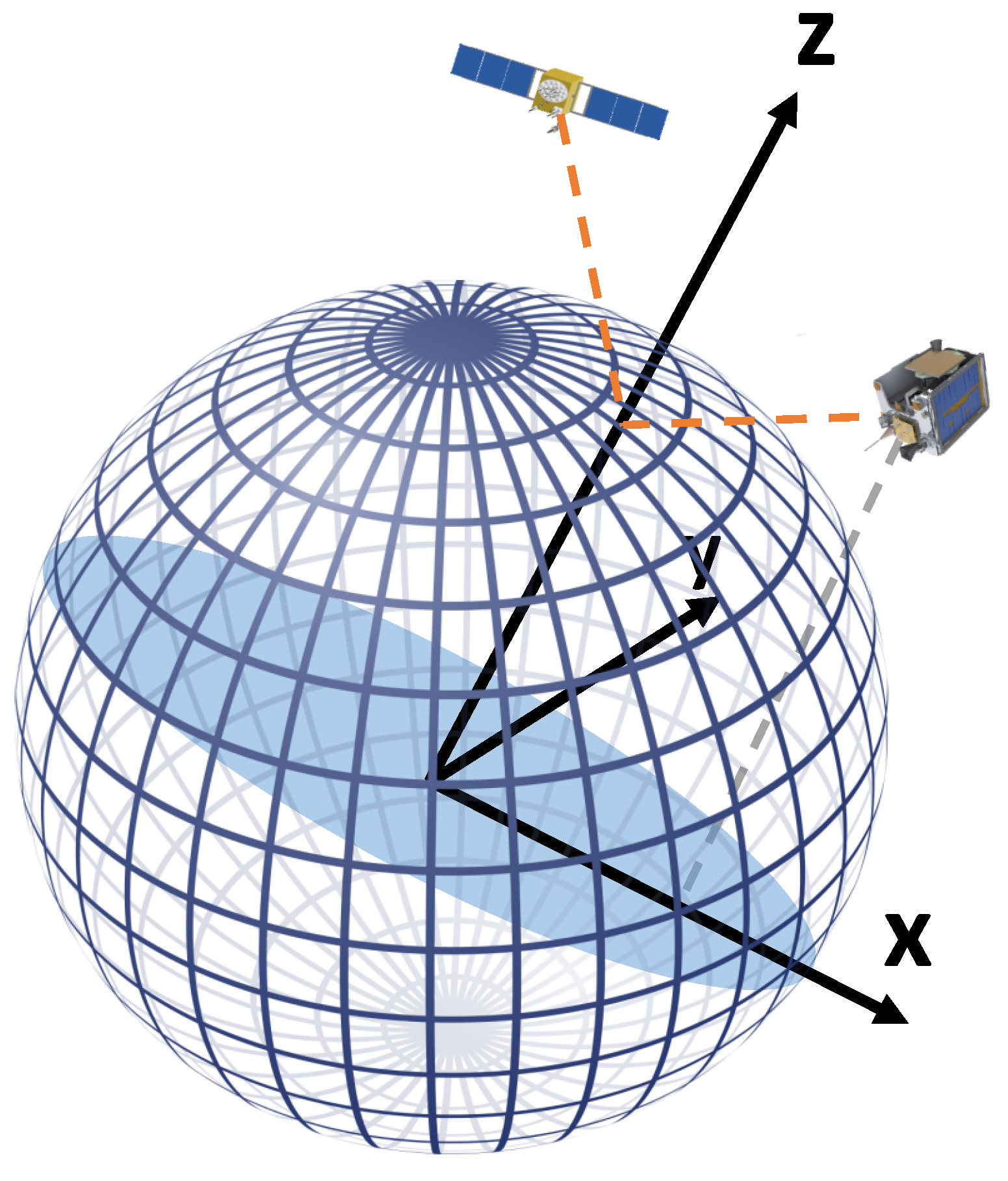
2.2.2. Transformation of the Vectors to the Model Reference Frame
To ease the simulation process, all of the position and velocity vectors are transformed to a model reference frame. The model reference frame is defined so that its origin is at the center of the Earth. The specular point is along the z-axis, and the x–y plane is parallel to the plane tangent to the surface at the specular point. The system is right-handed and the x-axis is toward the receiver satellite trajectory on the x–y plane. This reference frame is shown in
Figure 2.
To obtain the vectors in the model reference frame, they are first transferred to a local East, North, Up (ENU) coordinate system centered at the specular point. This transformations is as follows:
where
and
denote the geodetic longitude and latitude of the specular point, respectively. The ENU and the model refrence frame have equivalent
z components, while the the horizontal orientation can be different. With a rotation of the coordinate system with respect to
z-axis, ENU coordinates are transformed to the model reference frame. Then, the transformation of the horizontal components are first conducted with calculating the horizontal angular difference between the two systems:
where:
denoting the coordinates components of the reciever and trasnmitter satellite with
r and
t subscripts, respectively. Finally, the vectors in the model reference frame can be easily obtained:
and in the following, all of the vectors are designated in the model reference frame.
2.2.3. Establishment of the Glistening Zone
The glistening zone is considered as the area surrounding the specular point. So, a spherical plane is considered so that the curvature of Earth is taken into account. To this aim, a grid is etablished whose elements are designated in a 2D angular frame
. The components
and
are the angular differences with respect to the
z-axis of the model reference frame (intersecting the specular point), while the endpoints of the rays are at its origin. The boundary of the glistening zone can be considered as
, where
is the radius of the circular glistening zone. Finally, the grid elements can be obtained in the model reference frame by rotation of the specular point position
with respect to
y-axis and
x-axis as large as
and
, respectively:
where,
2.3. Power Distribution Calculation
In this step, the received power is calculated using Equation (
4). However, the direct calculation of the power map in the delay-Doppler domain is not possible unless it is first obtained in the spatial domain (over the established grid over ocean surface) and then mapped to the delay-Doppler domain afterward.
2.3.1. Power Distribution in the Spatial Domain
For each grid element we need the corresponding delay and Doppler shift values to calculate the received power scattered form that surface element. The delay refers to the time delays of the signal scattered from different grid elements. The delay value at every grid point on the ocean surface can be obtained using Equation (
9) and the path delay at the specular point (the minimum path delay) can be used to reference other paths across the grid. To be more specific, the C/A delay for each grind position vector
is obtained as:
where
Hz and
are the frequency of C/A code and the speed of light in a vacuum, respectively, and
P is given in Equation (
9). Finally,
is the delay with respect to the specular point.
The relative motion between the transmitter, receiver and grid elements cause the Doppler shift. In an arbitrary case, a signals Doppler frequency between two points
and
with velocity vectors of
and
, respectively, is as follows:
where
f is the signal frequency. In GNSS-R, the signal is received after being reflected and the total Doppler frequency at grid element
, after adding the rate of the receiver clock drift
, reads:
which can be rewritten as:
where
is the unit vector between the two points shown as the subscripts and
Hz is GPS L1 carrier signal frequency. The receiver clock drift is usually determined as an unknown parameter in positioning solutions. Nevertheless, this value is assumed zero in simulations of this study. In addition, the velocity of sea surface (grid elements) can be assumed equivalent to zero since its magnitude is much smaller than the transmitter and receiver satellites. This calculation is carried out at every grid element to map the scattered signal frequency over the glistening zone. Similar to delay computations, the Doppler frequency at the specular point is used to reference other frequencies across the grid as
.
2.3.2. Power Distribution in Delay-Doppler Domain
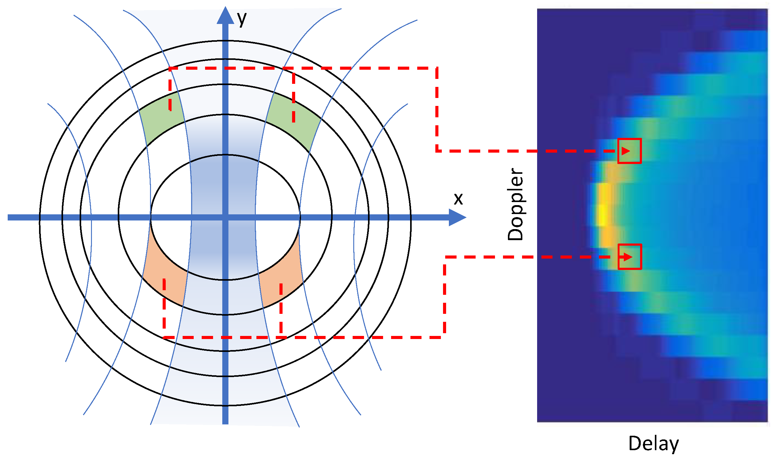
Once the power distribution is transformed from the spatial domain to the delay-Doppler domain, the simulated DDM is generated. To this aim, the relationship between the two domains must be first considered.
Figure 3 schematically illustrates an idealized DDM in both the spatial and delay-Doppler domain as well as the equi-Doppler curves, shown in blue, and the equi-range lines, ellipses in black. The right panel shows the corresponding DDM with the well-known horseshoe shape. The surface elements in the spatial coordinate domain, specified at the intersection of equi-range and equi-Doppler curves, and DDM pixels in the delay-Doppler domain are connected with a relation which is not one-to-one. In other words, every pixel of the DDM is not mapped to exactly one element of the spatial domain. Each DDM pixel is proportional to scattered power from the pair of pixels located symmetrically with respect to the intersection of the incidence plane with the ocean surface, which is the y-axis in the illustrated case. This is valid for every DDM pixel, except the pixel with maximum value, which normally corresponds to the specular point and the pixels with zero value (or a value close to the noise-floor), the dark blue area of the DDM in the right panel, which correspond to non-intersecting equi-range and equi-Doppler lines in the spatial domain. This non-one-to-one relation causes the so-called ambiguity problem.
Dealing with the quasi-specular scattering from the glistening zone and the discussed ambiguity, the received power can be spatially filtered with the help of the Woodward Ambiguity Function (WAF),
, applied as follows:
where * represents the two dimensional convolution operation and:
in which
is the area of the grid element. To accelerate the numerical simulations, Equation (
26), with the help of Fourier transformation
, can be rewritten as [
15]:
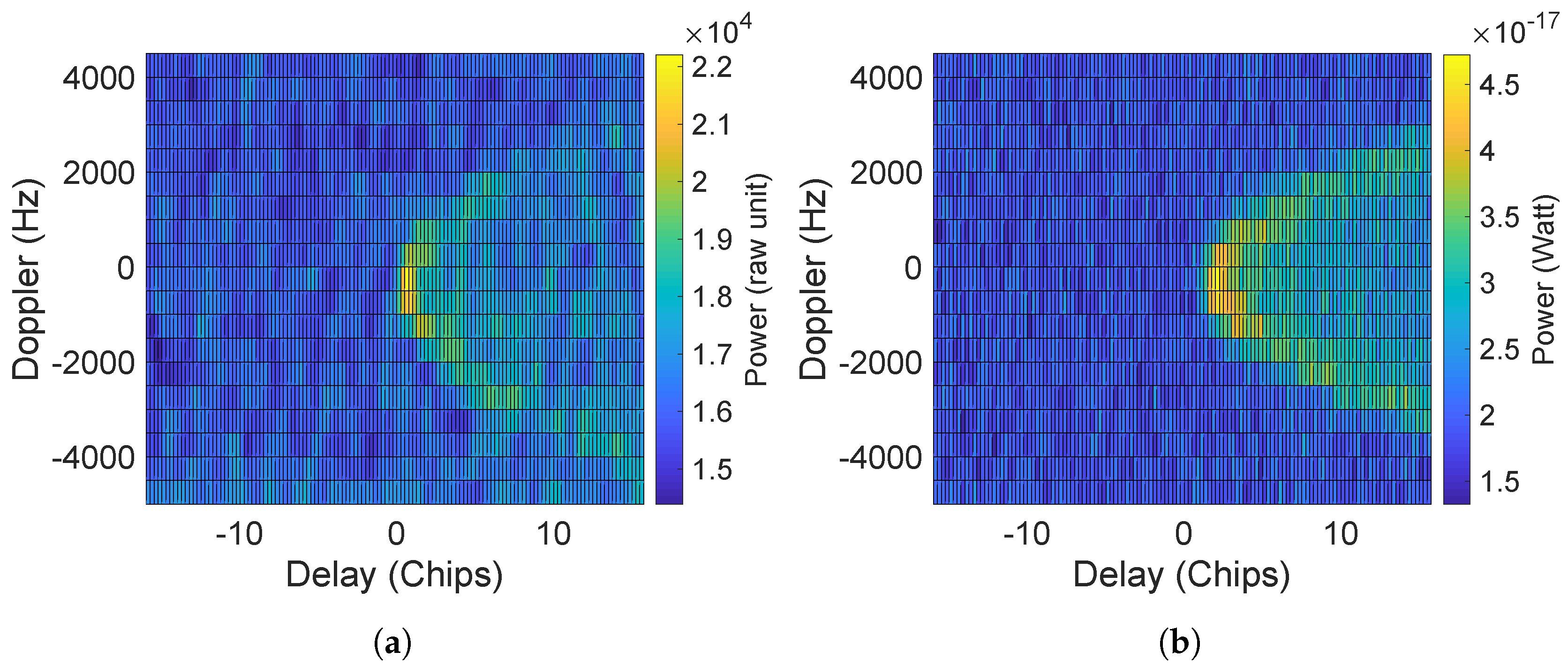
Finally, using the procedure described in this section, the DDMs are simulated for each scenario reported in
Table A1 and
Table A2.
Figure 4 shows a simulated and measured DDM onboard TDS-1.
4. Discussion and Conclusions
Rain attenuation, depending on the signal frequency, can affect the satellite scatterometric wind retrievals. This effect on the novel space-borne GNSS-R, providing wind information over oceans, needs to be characterized, since one of the main objectives of this technique is providing unaffected data during severe weather. Although the L-band GNSS signals are not attenuated at high levels by the raindrops in the atmosphere, the high condition number of GMFs at high wind speed ranges may result in a considerable bias in the resultant wind speed. In this study, the signal attenuation impact on the BRCS at the specular point as one of the important quantities derived from DDMs, as well as the bias in the wind speed, is evaluated. Empirical GNSS-R data analysis is impossible due to the lack of a sufficient number of observations at extreme wind speeds and rain rates. Consequently, this study is conducted simulating the DDMs from a satellite with orbital properties similar to TDS-1.
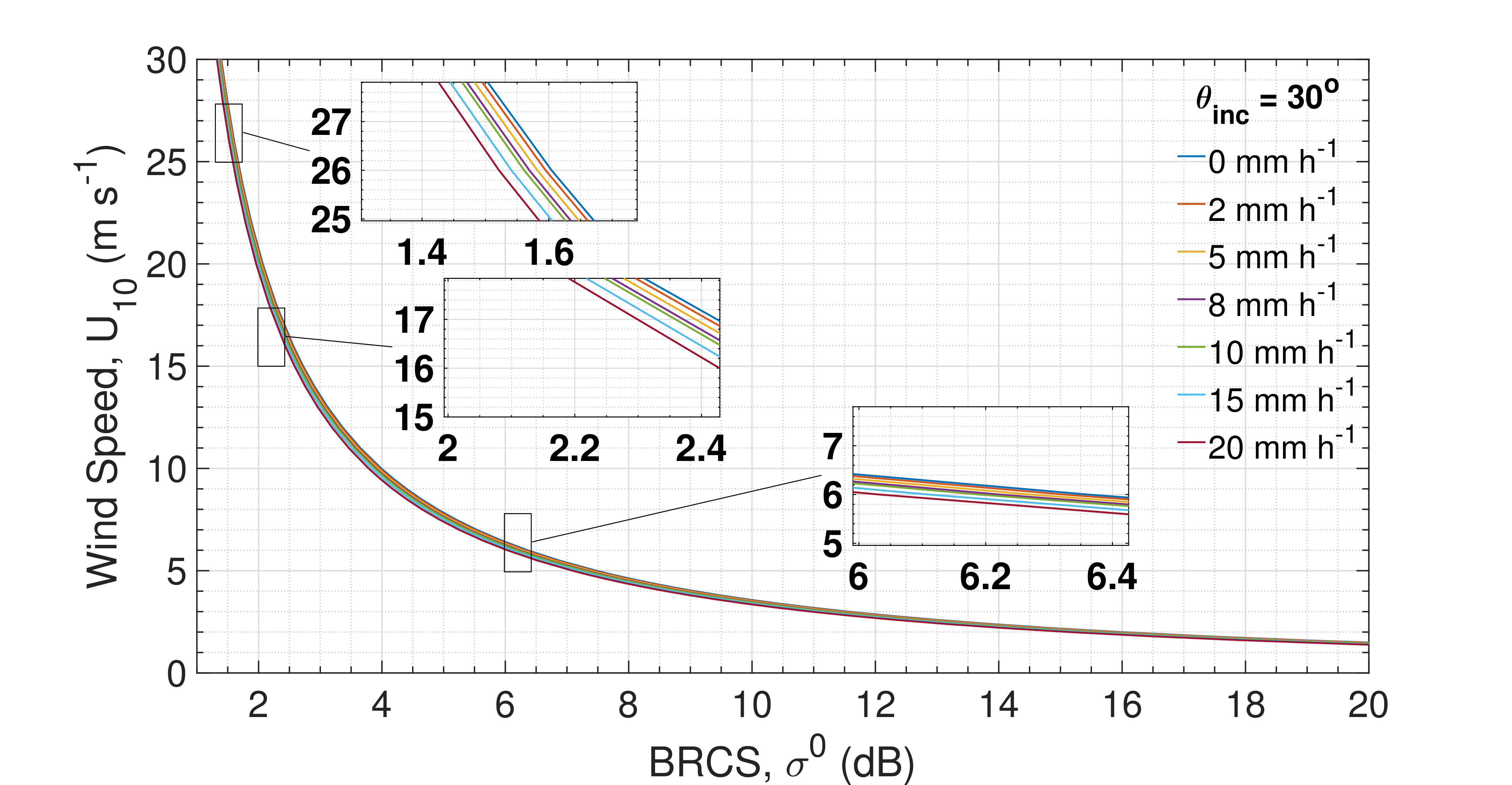
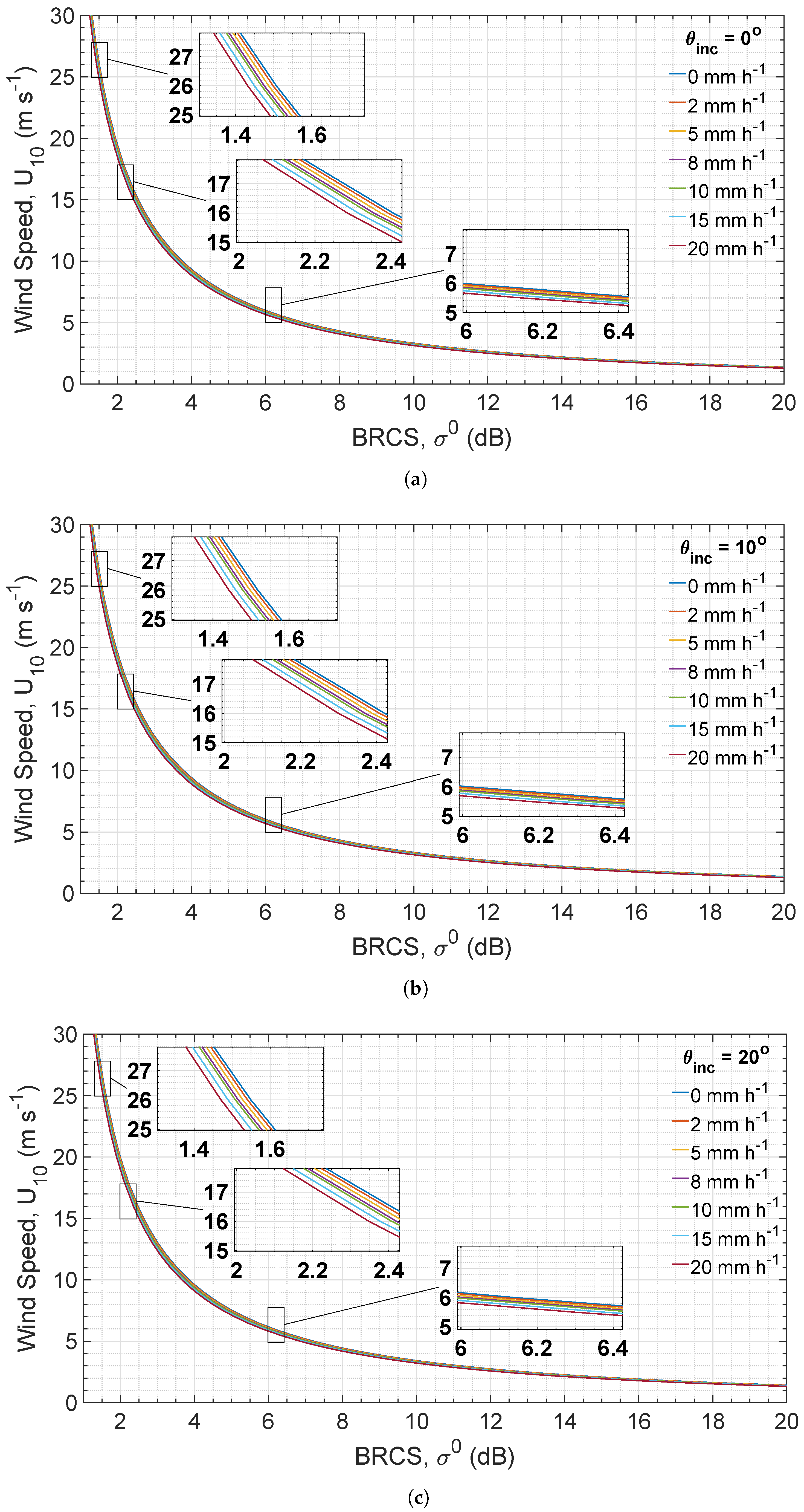
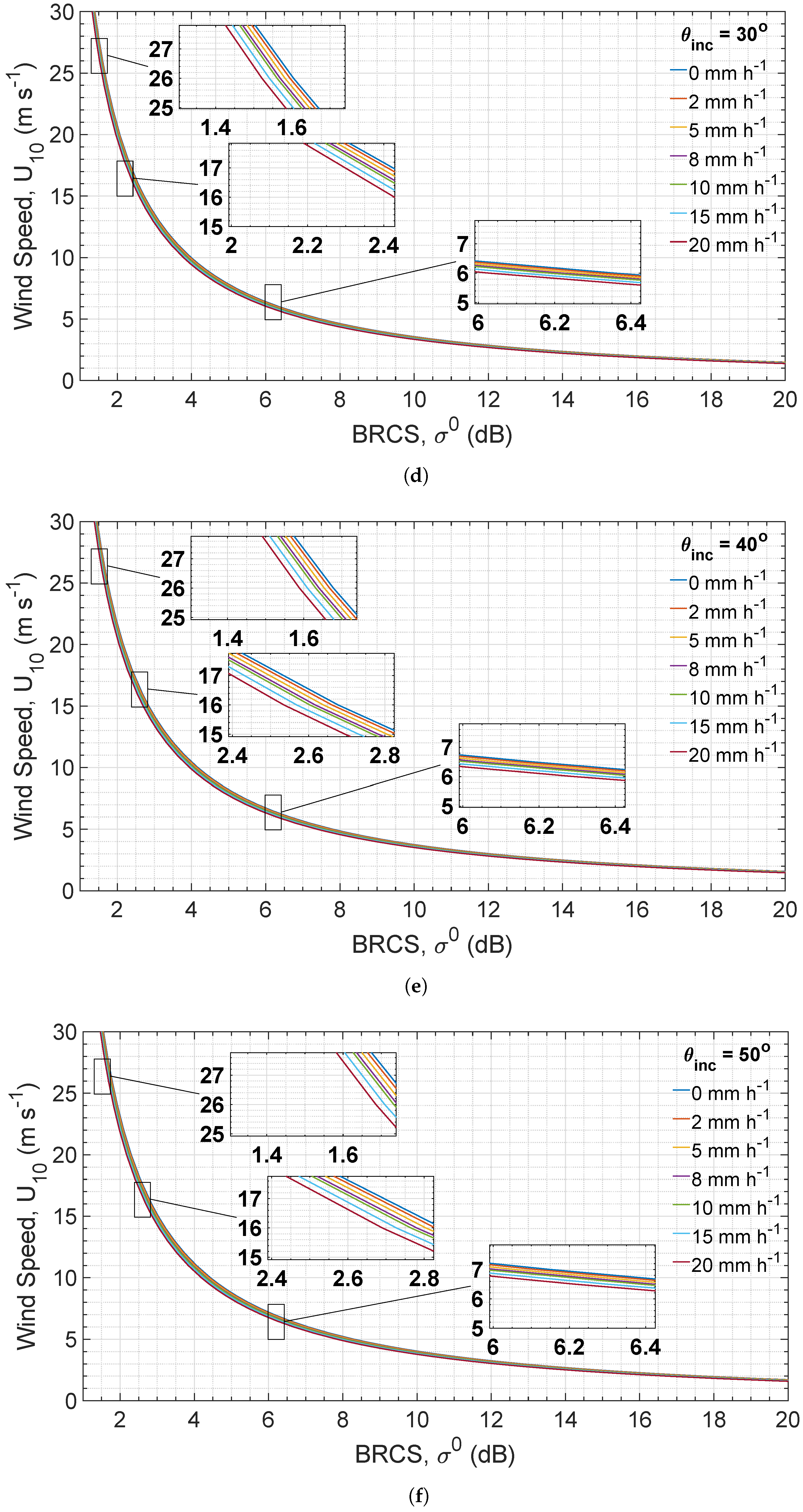
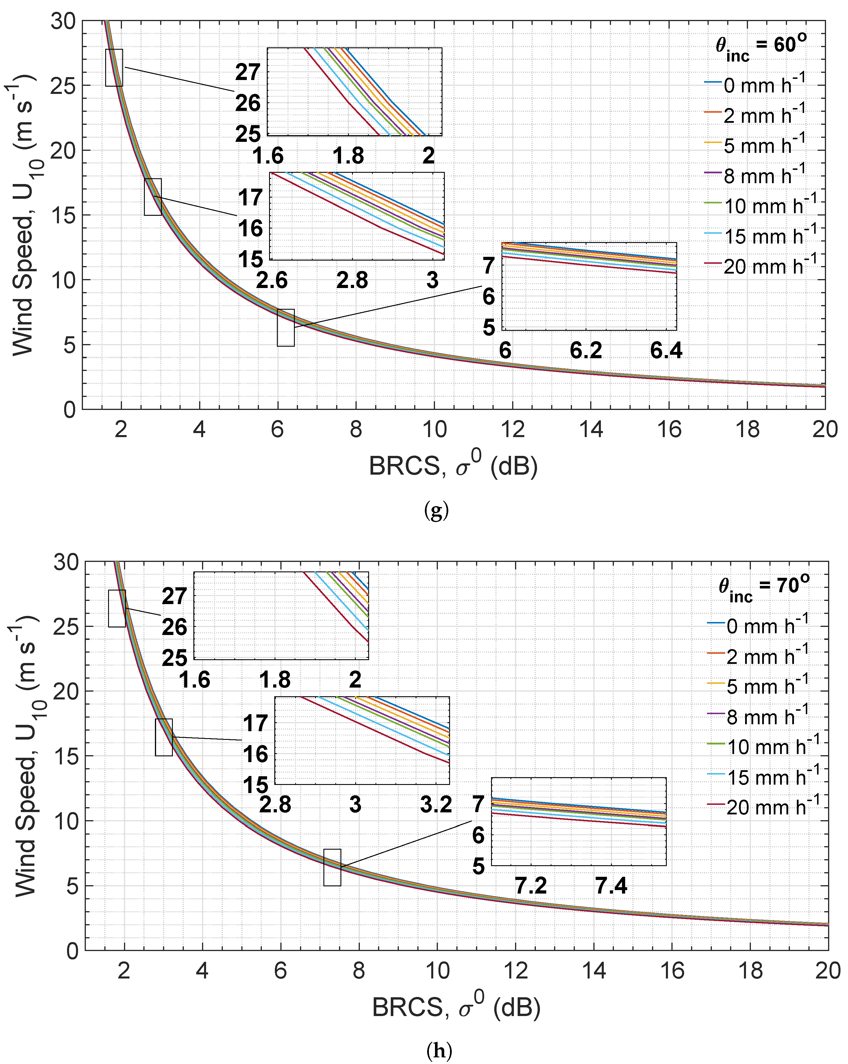
Figure 6 shows that the modification due to the rain attenuation is slight in at all of the incidence angles. As visualized in this figure (and as reported in
Figure 1 in terms of the condition number), at wind speeds below 5–10 m/s, the BRCS change over the wind speed is very gradual (d
d
is small) and the wind speed is barely responsive to BRCS changes. As a result, although the modifications in BRCS are relatively larger at low winds, the resultant bias is negligibly small (as shown in
Figure 7). At higher wind speeds, the slope of the curves in
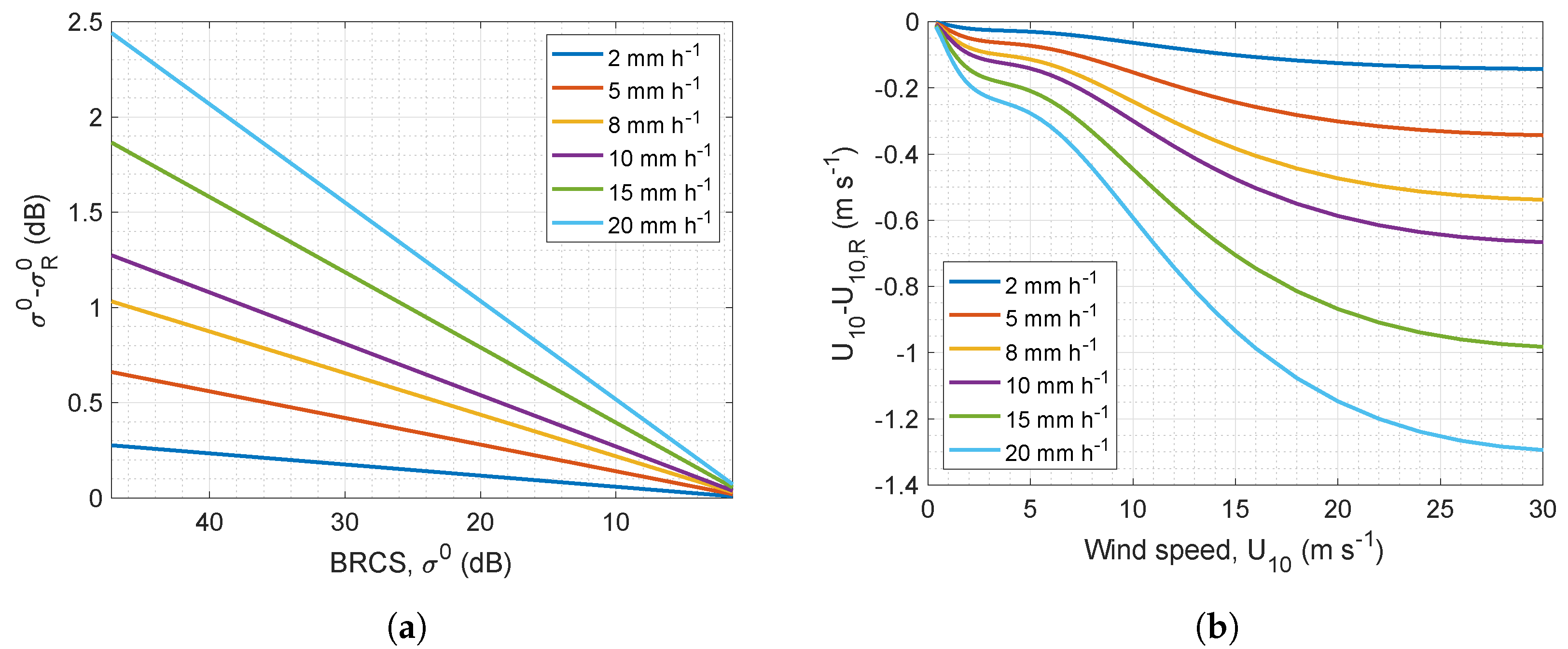
Figure 6 becomes very steep and small changes in BRCS correspond to relatively large changes in the derived wind speed. So, the component of wind speed error due to measurement error will be larger here. At typical precipitations (<5 mm/h), rain attenuation is negligibly ineffective so that at a wind speed of 30 m/s and incidence angle of 30°, the bias is smaller than ≈0.35 m/s (1%).
The numerical results demonstrate that rain rates of 10, 15 and 20 mm/h, might cause overestimation as large as ≈ 0.65 m/s (2%), 1.00 m/s (3%), and 1.3 m/s (4%), respectively, at a wind speed of 30 m/s and incidence angle of 30°. These statistics can be considerable if they exceed the required uncertainty threshold. This threshold is established considering the intrinsic errors in the wind speed retrieval algorithms, which represent the errors that would be still present even if the measurements were perfect. In practice, perfectly modeling the dependence of measured DDMs on non-wind variables is impossible and the algorithms are at a level of simplification. Such unavoidable error sources are combined with those from other phenomena, including the rain attenuation effect. The uncertainty threshold for CYGNSS mission is 2 m/s at wind speeds below 20 m/s and ±10% above 20 m/s. The errors shown in
Figure 7 are always much smaller than this threshold, and thereby might not be statistically significant, even at the incidence angle of 70°, which is the worst case scenario shown in
Figure 6.
In addition, according to [
28], the average rain rate during hurricanes is 3.9 mm/h and majority of the area (>50 %) are covered with a rainfall rate of 0.25–6.25 mm/h, estimated from composites of rain gauge data measuring rain rate on Pacific islands during passage of typhoons over a 21-year period. Only over 4% of the total covered area the rain rate is larger than 19 mm/h, which may be for a very short time (few minutes). In hurricane events, extremely large rain rates happen in connective cells which are highly localized and moving and evolving rapidly. So, the severe rainfalls happen for few minutes in fast-moving cells. However, the simulation here counts the rain attenuation effects very pessimistically. It considers constant and continuous precipitation along the entire path of the direct and reflected signal below the freezing height and over the entire glistening zone. The ambiguity function (explained in
Section 2.3.2) smooths the effect of rain attenuation over an area of ≈25 km. So, the effect of extreme rainfalls over small local regions can be significantly reduced. As a result, the effect of rainfall during hurricanes can be noticeably smaller in reality than the reported statistics.
It is recently demonstrated that rain splash altering ocean roughness can be considerable at low wind speeds. The characterization of the signal attenuation effect in this study complements the previous discussions and helps scientists obtain a better understanding in the development of models correcting rain effects on wind products and potentially in detecting rainfalls over oceans with GNSS-R measurements. Generally, this study demonstrates that rain attenuation effects can be ignored, considering the current technical and theoretical level of space-borne GNSS-R maturity, and the technique shows the required insensitivity to atmospheric rain attenuation for providing high-quality data from tropical storms.


