Article

Validation of Preliminary Results of Thermal Tropopause Derived from FY-3C GNOS Data

1
National Space Science Center, Chinese Academy of Sciences (NSSC/CAS), Beijing 100190, China
2
Beijing Key Laboratory of Space Environment Exploration, Beijing 100190, China
3
Joint Laboratory on Occultations for Atmosphere and Climate (JLOAC) of NSSC/CAS, Beijing 100190, China and University of Graz, 8010 Graz, Austria
4
University of Chinese Academy of Sciences, Beijing 100049, China
5
State Intellectual Property Office of the P.R.C, Beijing 100088, China
*
Author to whom correspondence should be addressed.
Remote Sens. 2019, 11(9), 1139; https://doi.org/10.3390/rs11091139
Submission received: 15 April 2019 / Revised: 1 May 2019 / Accepted: 10 May 2019 / Published: 13 May 2019

Abstract

:
The state-of-art global navigation satellite system (GNSS) occultation sounder (GNOS) onboard the FengYun 3 series C satellite (FY-3C) has been in operation for more than five years. The accumulation of FY-3C GNOS atmospheric data makes it ready to be used in atmosphere and climate research fields. This work first introduces FY-3C GNOS into tropopause research and gives the error evaluation results of long-term FY-3C atmosphere profiles. We compare FY-3C results with Constellation Observing System for Meteorology, Ionosphere and Climate (COSMIC) and radiosonde results and also present the FY-3C global seasonal tropopause patterns. The mean temperature deviation between FY-3C GNOS temperature profiles and COSMIC temperature profiles from January 2014 to December 2017 is globally less than 0.2 K, and the bias of tropopause height (TPH) and tropopause temperature (TPT) annual cycle derived from both collocated pairs are about 80–100 m and 1–2 K, respectively. Also, the correlation coefficients between FY-3C GNOS tropopause parameters and each radiosonde counterpart are generally larger than 0.9 and the corresponding regression coefficients are close to 1. Multiple climate phenomena shown in seasonal patterns coincide with results of other relevant studies. Our results demonstrate the long-term stability of FY-3C GNOS atmosphere profiles and utility of FY-3C GNOS data in the climate research field.

Graphical Abstract

1. Introduction

The tropopause region plays an important role in the earth’s atmosphere because of the interior exchange of substances and energy between stratosphere and troposphere [1], which is closely associated to deep convection and the Brewer–Dobson circulation [2]. Thus, the variation of tropopause structure may affect the stratospheric moisture content and stratospheric chemistry [3,4]. Also, the variation of tropopause parameters relates to the anthropogenic impact on the environment, and thus tropopause parameters can be regarded as an indicator of the effect of human activities on the environment [5]. The robust increase of tropopause height is believed to be in response to the increasing amount of carbon dioxide emissions, which leads to the warming in the troposphere and the cooling in the stratosphere, decreasing the stability of the tropopause [5,6]. Furthermore, tropopause height is correlated with stratospheric ozone content. Steinbrecht et al. [7] analyzed the relationship between tropopause height and local ozone content, indicating that the global uptrend of tropopause height is corresponding to the ozone depletion in the stratosphere. The emission of carbon dioxide and the global warming, as well as the variation of tropospheric and stratospheric ozone content are closely connected with human activities. Therefore, monitoring tropopause parameters is meaningful for not only atmosphere and climate research, but also human life [8].
The traditional methods to observe tropopause are based on ground-based observation, such as the radiosonde and LIDAR, and numerical models, like re-analysis field. However, the former is restricted by the terrain and heavy cost and thus it cannot provide global-covered data, and the latter suffers from coarse resolution [9] and not able to furnish real-time data [10,11]. The advent of the global navigation satellite system (GNSS) radio occultation (RO) technique makes up for the shortcomings of traditional observation methods. Its unique properties, such as high global coverage, high vertical resolution and long-term stability, enable it to be a powerful tool for detection of the tropopause. Those advantages are extremely obvious when monitoring rapidly changing variances such as tropopause changes caused by tropical cyclones, which is well discussed by Biondi et al. and Ravindra et al. [12,13]. Furthermore, the number of RO events will increase with the launching of RO missions, which leads to a growing number of RO atmosphere profiles.
RO data was introduced into the tropopause research field immediately after the success of the proof-of-concept Global Positioning System/Meteorology (GPS/MET) mission. Nishida et al. and Randel et al. [14,15] first used GPS/MET data to analyze the structure of the tropical tropopause region. With the development of new RO missions and the accumulation of RO data, Schmidt et al. [16] illustrated a clear quasi-biennial oscillation of temperature variation upon the tropopause over the equator by using three-year data of Challenging Mini-satellite Payload (CHAMP) mission. Meanwhile, Schmidt et al. [17] first studied the global tropopause parameters via four-year CHAMP data and auxiliary Satellite de Aplicaciones Cientificas-C (SAC-C) data. Similarly, Schmidt et al. [18] declared a global uptrend of tropopause height about 4–7m/year. After the accumulation of Constellation Observing System for Meteorology, Ionosphere and Climate (COSMIC) data, Kim and Son, and Son et al. [19,20] used COSMIC data to analyze the structure and the variation of global thermal tropopause. In recent years, Rieckh et al. [21] used 2001–2013 atmospheric data from multiple RO missions to study characteristics of multi-tropopause and the correlation between the El Niño southern oscillation and quasi-biennial oscillation, and Li et al. [22] compared the 12 years of tropopause parameters derived from multiple RO missions.
China’s GNSS occultation sounder (GNOS) onboard the FengYun 3 series C (FY-3C) satellite was designed and developed by National Space Science Center, Chinese Academy of Sciences (NSSC, CAS), for sounding the Earth’s neutral atmosphere and ionosphere [23]. The FY-3C satellite was launched in September 2013, flying in a sun-synchronous polar orbit of inclination 98.8°, mean altitude 836 km and orbital period 101.5 min [24]. The onboard state-of-the-art RO sounder, GNOS, is compatible for both BeiDou navigation satellite system (BDS) signal and Global Position System (GPS) signal [23,25,26]. The main scientific missions undertaken by FY-3C GNOS are as follows: to provide continuously available global atmosphere profiles for weather forecast, global climate monitoring and atmospheric research; to provide ionosphere profiles for ionosphere research, geomagnetism, radio communication and space science research; and to obtain the precursor information of natural disasters and improve the disaster forewarning capabilities [27]. The following FY-3 series of operational meteorological satellites will continue to carry GNOS as one of the major payloads. Besides, the FY-3D satellite has already been launched in November 2017, which is now at the stage of test in-orbit.
Until now, FY-3C has been in operation for more than 5 years, providing about ten thousand atmosphere profiles per month. As a sun-synchronize satellite, the local time distribution of FY-3C RO events are centered at 10 am and 10 pm, which provides time-centered observation [28]. After 5 years of data accumulation, FY-3C GNOS (FY-3C in later sections) data are ready to be used in the climate research field. This work first introduces FY-3C data into climate research, with the purpose of validating FY-3C atmosphere profiles and demonstrating the utility of FY-3C data in tropopause climate research. To achieve above points, we validate the FY-3C temperature profiles and derived tropopause parameters to give a long-term data accuracy evaluation and show the error characteristic. We also discuss the spatial-temporal variation of tropopause parameters derived from FY-3C data and compare tropopause variation regularities with results of other relevant studies so as to confirm the climate research utility of FY-3C data. FY-3 series satellites, current C, D and future E, F, G, R, will provide more than 10 years continues RO data, which will meet the demand of climate research. This work is the first step for the assimilation of FY-3 series data into atmosphere and climate research fields.
We first give a description of data and the tropopause discrimination method and then present the comparison result of different data sources. After the check of FY-3C tropopause parameters, the spatial-temporal variations of global tropopause parameters derived from FY-3C data are illustrated. At the end, conclusions are summarized.

2. Materials and Methods

In this work, we used dry temperature profiles to retrieve tropopause height and tropopause temperature, because in the tropopause region (7–18 km according to different latitude), the effect of water vapor on temperature is insignificant and the retrieval of dry temperature profiles needs no auxiliary data.

2.1. RO Data

Except for the missing FY-3C data during May 2015 due to satellite debugging, dry temperature profiles of FY-3C and COSMIC from January 2014 to December 2017 were used in this work. Temperature profiles of FY-3C were retrieved, with the vertical resolution of 90–120 m in the range of 7–25 km altitude. COSMIC temperature profiles provided by UCAR COSMIC Data Analysis and Archive Center (CDAAC) were download from cdaac-www.cosmic.ucar.edu, whose vertical resolution is 30–40 m in the range of 7–25 km altitude.
The latitudinal distribution of temperature profiles of two missions is shown in Figure 1. Here we binned temperature profiles into 36 latitude bands, from 90N to 90S, which means each latitude band was of 5 degrees. The top panel in Figure 1 demonstrates the same latitudinal distribution of both 4 years of FY-3C and COSMIC temperature profiles. The largest data density for FY-3C and COSMIC were of 15,000 and 50,000 per 5° latitude band around 20° and 50° in both the Southern hemisphere and the Northern hemisphere and the smallest data density for both RO missions were less than 5000 and 20,000 per 5° latitude band in the tropics and polar regions, respectively. In total, the amount of FY-3C temperature profiles was approximately one-third of the number of COSMIC temperature profiles. The bottom panel describes the temporal distribution of RO temperature profiles. FY-3C provided more data in the second half of the year, which was contrasted with the distribution of COSMIC data.

2.2. Radiosonde Data

With respect to radiosonde data, we choose nine stations which were distributed in different latitude in the Northern hemisphere. Temperature profiles of six stations were Vaisala RS92 version-2 level-2 radiosonde data obtained from the Global Climate Observing System (GCOS) Reference Upper-Air Network (GRUAN), with a very high vertical resolution of 10–30 m from land surface to 25 km altitude. Temperature profiles of the other three stations were IGRA version-2 level-2 radiosonde data, downloaded from www.ncdc.noaa.gov. Compared with GRUAN RS92 data, IGRA data had good temporal stability, with two temperature profiles in each day, but the vertical resolution of the chosen IGRA data was lower than RS92 data, about 80–100 m from land surface to 25 km altitude. Table 1 gives the detailed information of these radiosonde stations, and Figure 2 depicts the distribution of the radiosonde stations. The names of three IGRA stations were too long, thus we use their first three letters in later sections.
Although there are hundreds of stations in the global archive, only a few stations met our demand because the distribution and the quality of stations were uneven, and the radiosonde data needed to have enough collocated pairs with FY-3C data. Data of GRUAN stations were of high quality, with only few extreme values or invalid values, and thus we mainly used this kind of radiosonde data. We finally chose six of 17 stations’ data from their website (ftp.ncdc.noaa.gov/pub/data/gruan/processing/level2/RS92-GDP/version-002/) for they had enough collocated pairs and were well distributed in different latitudes. Most of IGRA stations’ data were of 2 km vertical resolution, which cannot be used in tropopause research, and we chose three suitable IGRA stations as supplements to add samples in tropics.

2.3. Tropopause Determination Method

To define thermal tropopause, there are mainly three methods: cold point method, bending angle method, and temperature lapse rate method. Cold point method is to regard the coldest point in the temperature profile as the tropopause point (below 20 km). This method was easy to apply, but it was only applicable for the tropical tropopause because compared with the other two methods, this method usually led to higher tropopause heights (TPHs) in mid and high latitude regions [29] and sometimes it was hard to find tropopause in high latitudes due to the almost monotone decreasing temperature profile caused by polar vortex. Bending angle method [30] could avoid additional RO data processing and physical assumptions, such as hydrostatic equilibrium, and this method showed good agreement with temperature lapse rate method [31]. However, compared with the lapse rate method, the computational efficiency of the bending angle method was relatively low. Temperature lapse rate method is commonly used for its simple procedure and universal applicability, which allows comparison to other studies. We thus used the World Meteorological Organization (WMO) tropopause definition to compute TPH and tropopause temperature (TPT). According to the WMO (1957), the tropopause height is defined as the lowest level at which the lapse rate decreases to 2 °C/km or less, also provided the average lapse rate between this level and all higher levels within 2 km does not exceed 2 °C/km.

2.4. Algorithm Introduction

The tropopause algorithm was based on the lapse rate method, however, because of the dry temperature profiles used in this work, the bottom limits needed to be set to avoid the effect of high concentrations of water vapor in the lower troposphere. The bottom limits were based on empirical analysis and results from other relevant studies [21,32]. We set the bottom limit to a constant of 12 km for tropics ([30S, 30N]) during the whole year, and to 6 km and 5 km for high latitude regions ((60S, 90S] (60N, 90N]) in summer (JJA) and winter (DJF). Considering the TPH latitudinal and temporal variation, we set the bottom limits that changed linearly with latitude and month during spring (MAM) and autumn (SON) in mid ((30S, 60S] (30N, 60N]) and high latitude regions, which are as follows:
B M S = 8 ( | L a t | 30 ) / 15
B M W = 7 ( | L a t | 30 ) / 15
B H S A = 6 | M o n 7 | / 6
B M S A = B M S ( B M S B M W ) × | M o n 7 | / 6
B M S , B M W and B M S A represent the bottom limits for mid latitude regions in summer, winter and spring/autumn, respectively, and B H S A represents the bottom limit for high latitude regions during spring or autumn. Lat and M o n correspond to the latitude and month of temperature profiles, and for the latitude, northern latitude is positive and southern latitude is negative.
Equation (1) and Equation (2) were used to calculate the bottom limits of mid latitude regions during summer and winter, respectively. Equation (3) is for high latitude regions during spring and autumn, while Equation (4) is for mid latitude regions during spring and autumn. Spatially, this piecewise function is discontinuous at 30S and 30N, and temporally, this function is discontinuous at the start and the end of summer and winter.
In addition, we set the top limit to 22 km in the tropics and mid-latitude regions, and 15 km in high latitude regions to exclude abnormal results. For ease of comparison, we interpolated all temperature profiles with 100 m intervals.

2.5. Binning Method

In the comparison of temperature profiles and tropopause parameters between two RO missions, we binned the data into five latitude bands, 90N–60N, 60N–30N, 30N–30S, 30S–60S, 60S–90S to give a global validation of FY-3C data. To investigate global tropopause parameters, we first calculated tropopause for each temperature profile, then estimated the mean values of tropopause as regional tropopause values, and thus in consideration of the amount of FY-3C RO data, we set 5° × 10° (latitude × longitude) bins centered at 87.5N–87.5S (36 latitudes) and 175E–175W (36 longitudes) to ensure the resolution and the smoothness of global TPH and TPT. In each band, if any TPH value occured more than three times standard deviation from the mean TPH value, these TPHs were regarded as error values and were excluded with its corresponding TPTs.

3. Results

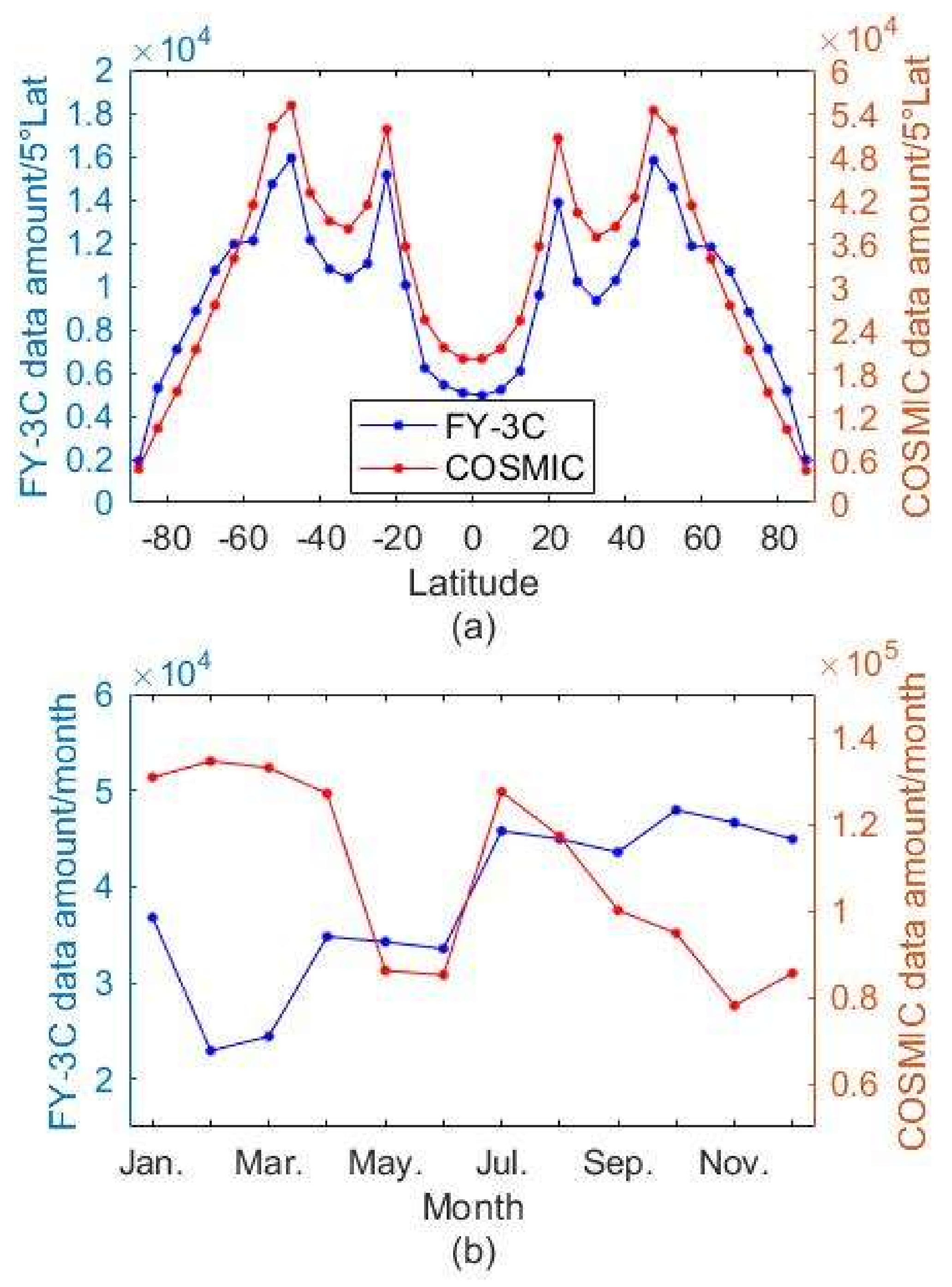
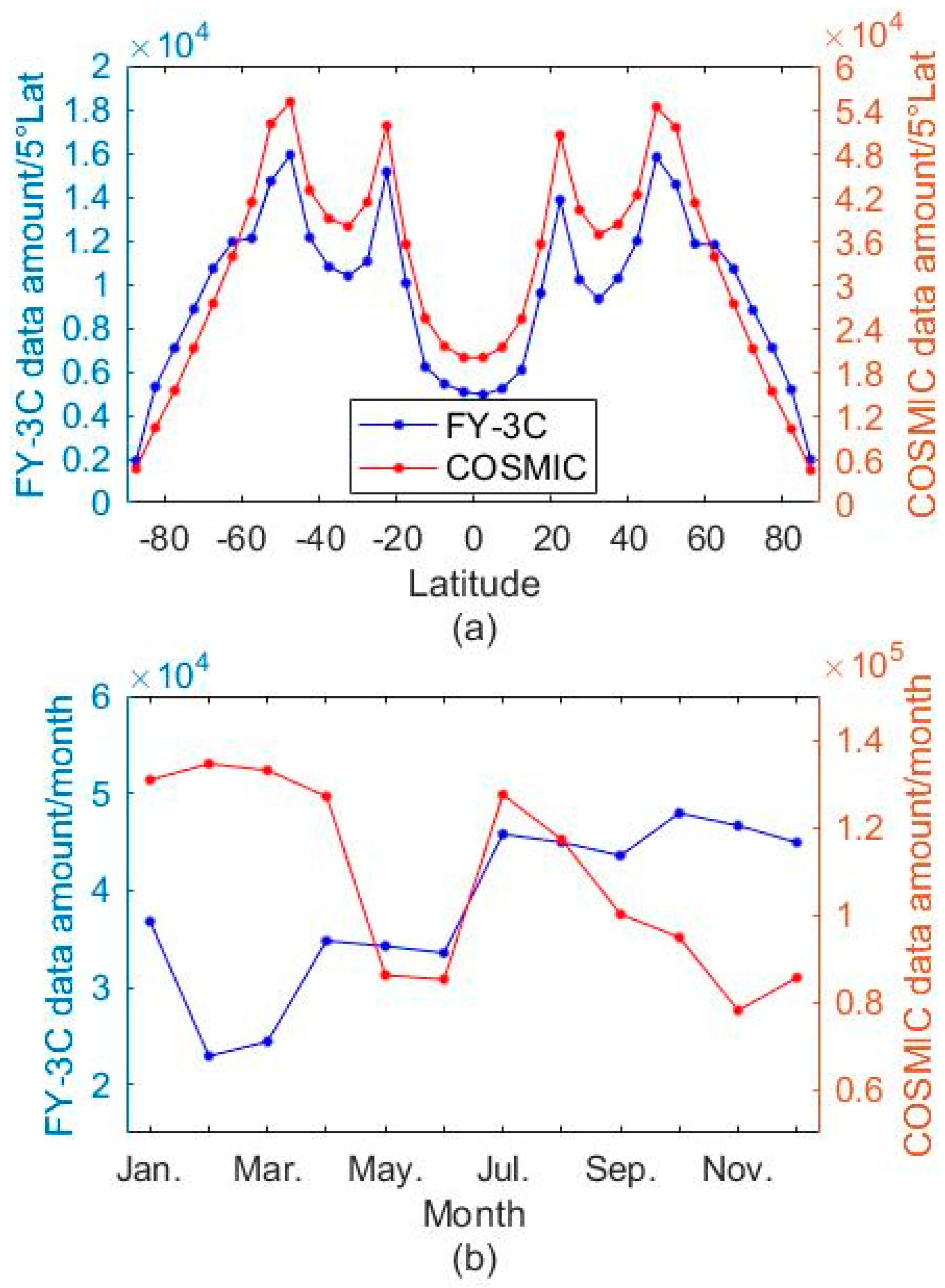
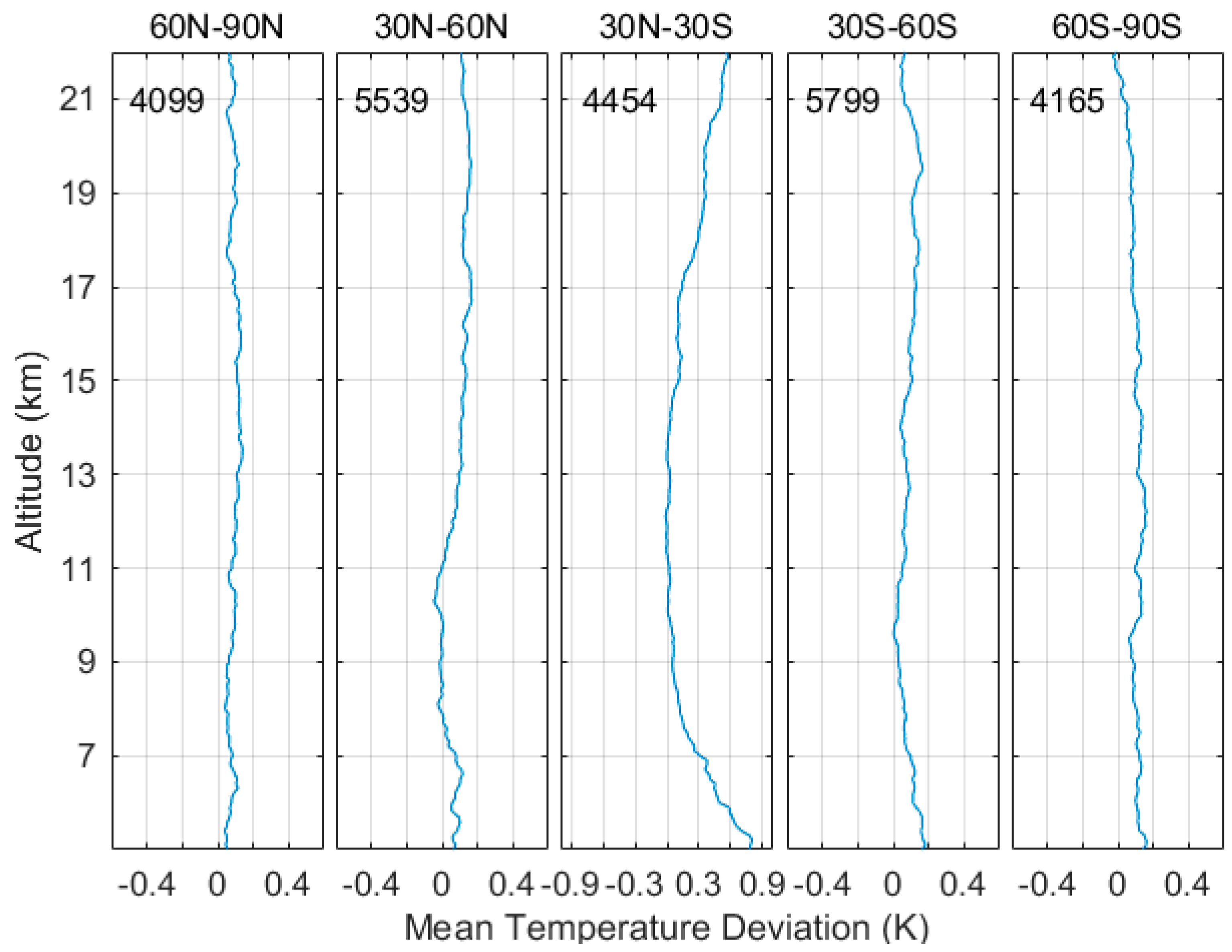
3.1. Temperature Comparison with COSMIC Data

Before the comparison of tropopause parameters, we first validated the mean temperature deviation and the root mean square error between collocated pairs of COSMIC and FY-3C data. The criterion of the collocated pair in this work was that the time interval was less than 3 h and the distance between two profiles was less than 300 km. To calculate mean temperature deviation, we interpolated both FY-3C and COSMIC temperature profiles in a 5 km to 25 km range with the interval of 100 m which was similar to the vertical resolution of FY-3C temperature data. The computational process was as follows:
Δ T r e g i o n ( h ) = 1 N r e g i o n ( C S T r e g i o n ( h ) F Y T r e g i o n ( h ) )
R M S T r e g i o n ( h ) = 1 N r e g i o n ( C S T r e g i o n ( h ) F Y T r e g i o n ( h ) ) 2
where Δ T r e g i o n ( h ) and R M S T r e g i o n ( h ) represent the mean temperature deviation and the root mean square error at altitude level h in different latitude bands, respectively; N r e g i o n represents the number of collocated data pairs in different latitude bands; C S T r e g i o n ( h ) and F Y T r e g i o n ( h ) represent the temperature value of COSMIC data and corresponding FY-3C data at altitude level h in different latitude bands, respectively.
The comparison results are illustrated in Figure 3 and Figure 4. Overall, COSMIC temperature data were slightly higher than collocated FY-3C temperatures, and the mean temperature deviation was less than 0.2 K in mid and high latitude regions. In the tropics, owing to the decreasing RO measuring error caused by high concentration of water vapor that reduced the signal strength and increased the signal instability, the dry temperature difference reduced rapidly from 5 km to 8 km, towards zero from 8 km to 17 km, and then gradually increased with altitude. The temperature root mean error was holistically less than 2 K, except for 5–8 km and 17–22 km in tropics, which was similar to the trend of mean temperature deviation.

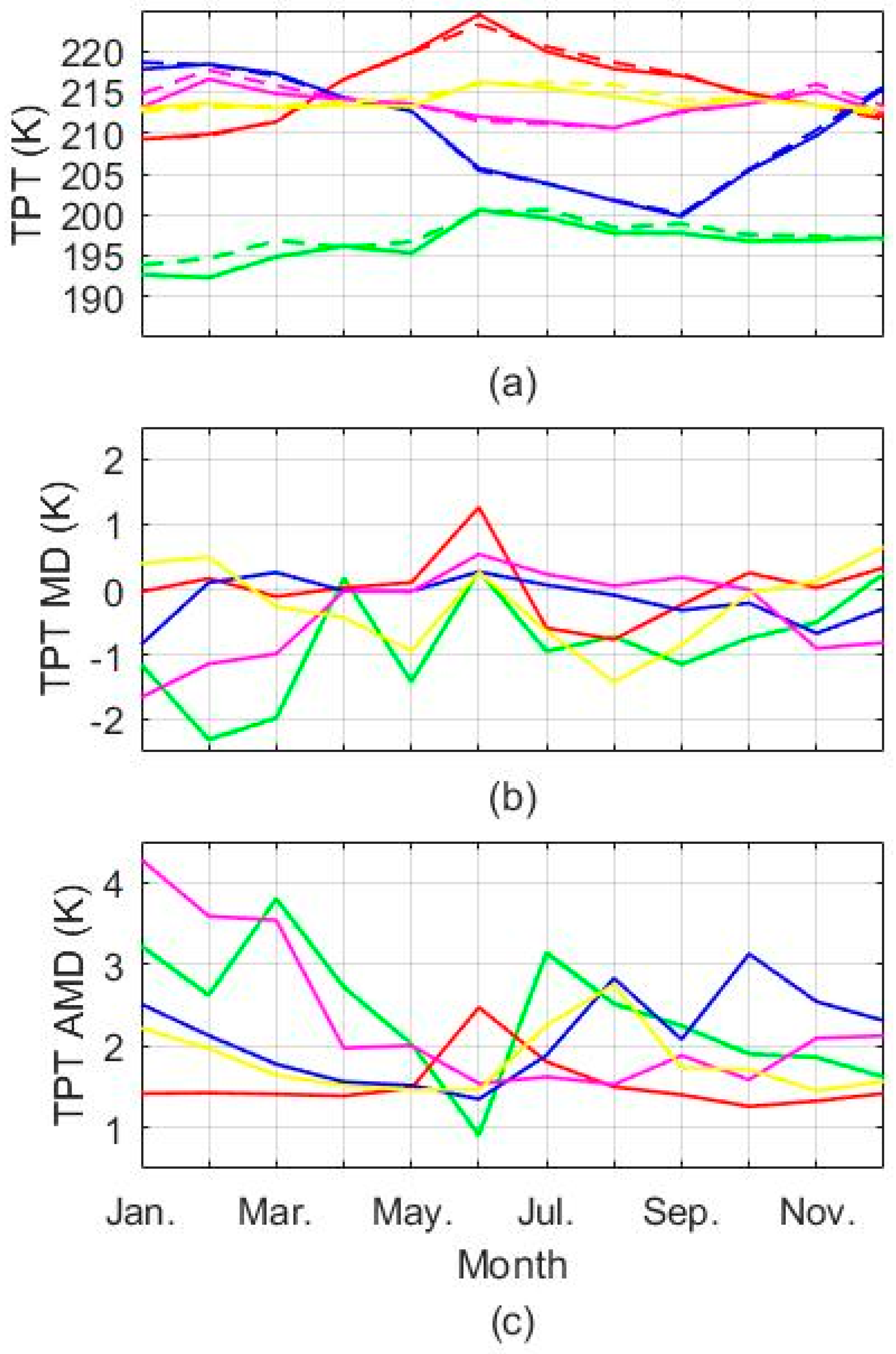
3.2. Tropopause Parameters Comparison with COSMIC Data

After the validation of FY-3C temperature profiles, the annual cycle average TPH and TPT derived from 2014–2017 collocated FY-3C and COSMIC temperature profiles were compared. To discuss the bias objectively, we present both mean deviation (MD) and absolute mean deviation (AMD) for TPH and TPT comparison. MD and AMD were calculated as follows:
MD = 1 N ( F Y 3 C C O S M I C ) )
AMD = 1 N | F Y 3 C C O S M I C |
where N represents the number of collocated pairs; F Y 3 C and C O S M I C represent their collocated TPT or TPH data.
Figure 5 describes the annual cycle mean TPHs and the TPH bias, indicating that the majority of FY-3C TPHs were less than 100 m higher than collocated COSMIC counterparts and the TPH AMD were mainly less than 300 m, except for 60S–90S during July to November. The difference of annual cycle mean TPTs was more obvious than that of annual cycle mean TPHs. In Figure 6, TPTs derived from FY-3C were about 1 K lower than TPTs derived from COSMIC, which checked with the result of annual cycle TPHs. The obvious bias appeared on tropic and mid latitudes in the Southern hemisphere during January to March, where the TPT MD was smaller than –2 K and TPT AMD was larger than 3 K.

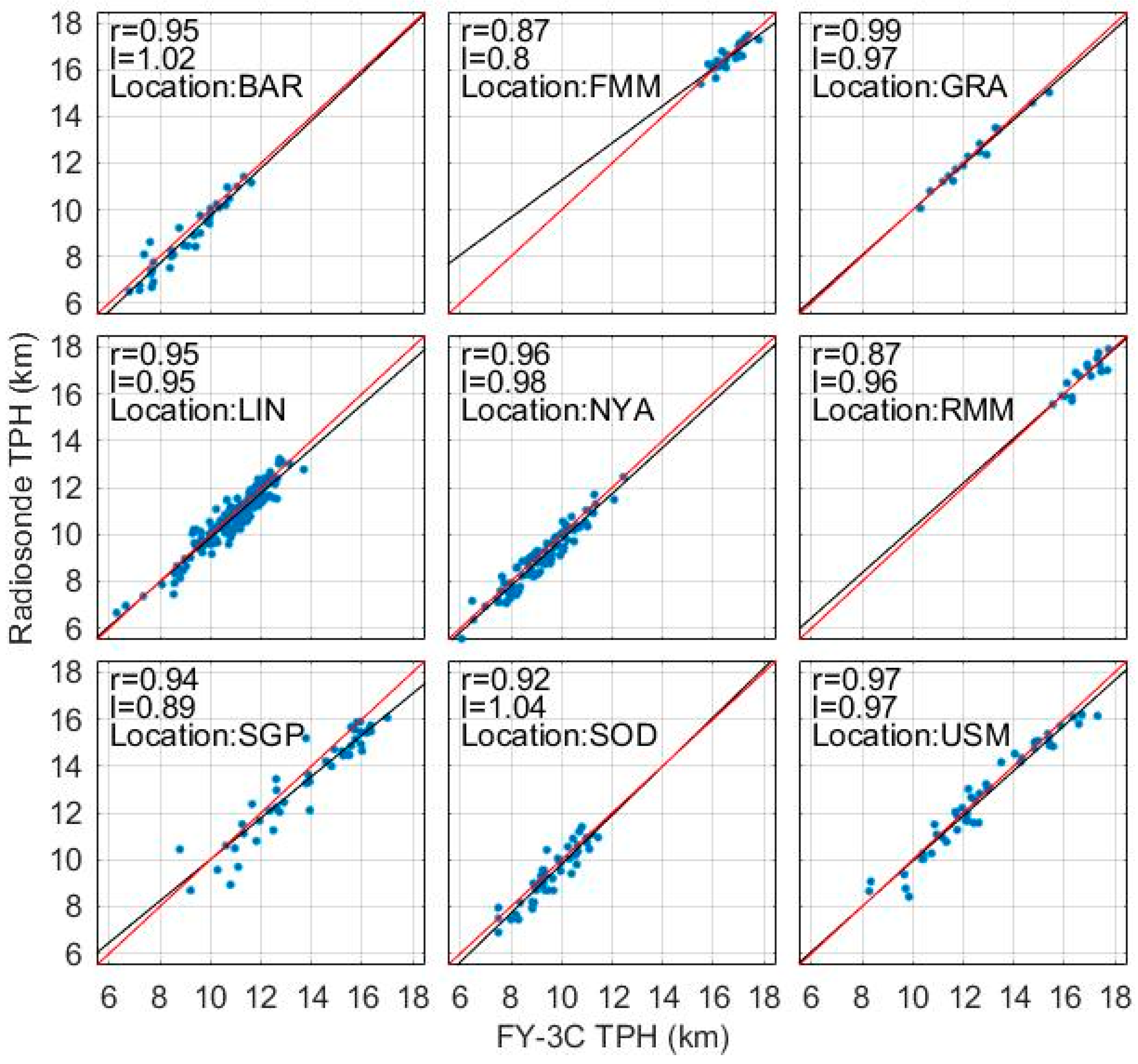
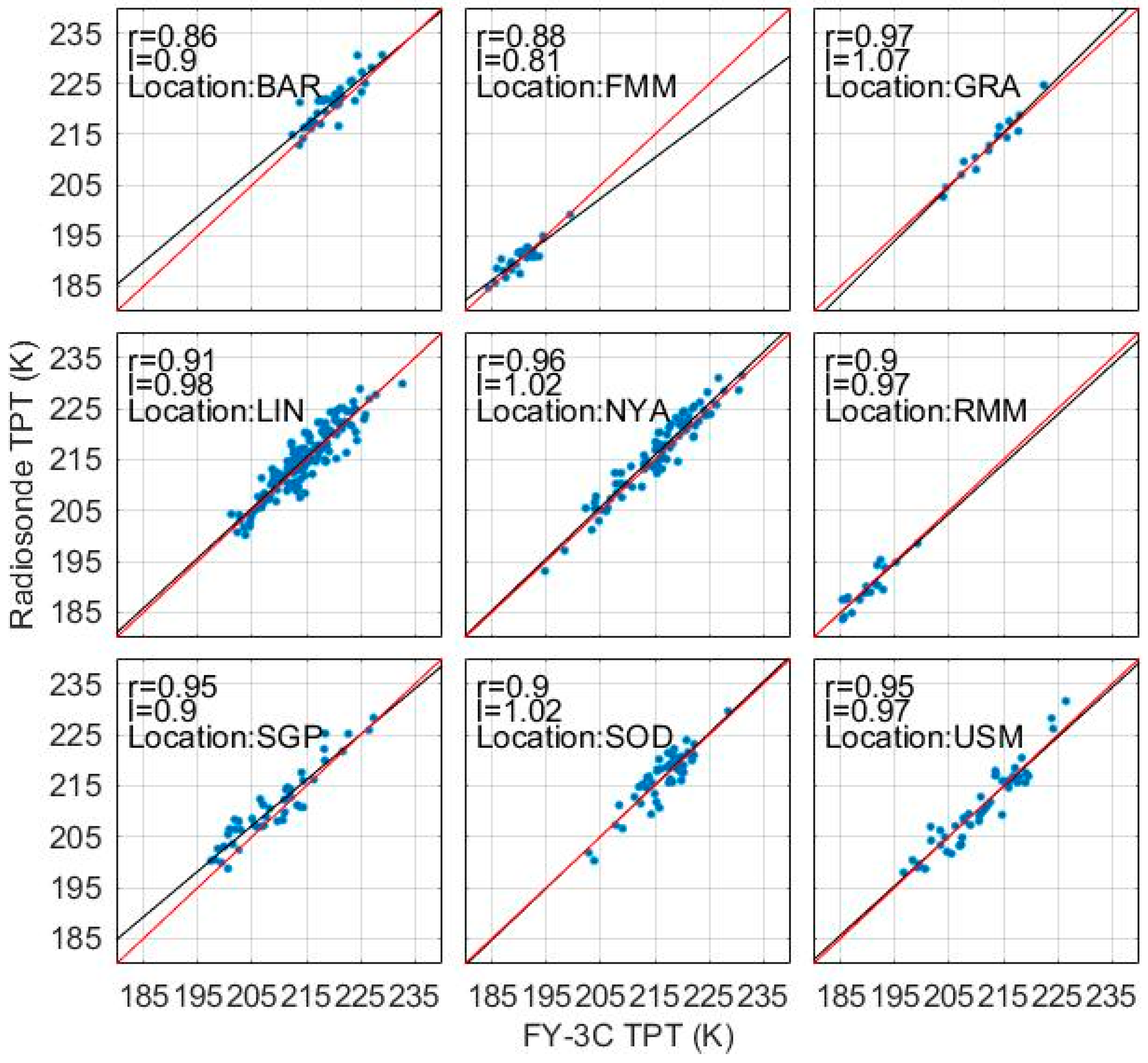
3.3. Tropopause Parameters Comparison with Radiosonde Data

This subsection describes the comparison result of tropopause parameters between FY-3C and radiosonde. To obtain objective comparison results, we focused on tropopause parameters derived from the collocated temperature profile pairs of FY-3C and nine different latitude radiosonde stations. The collocate criterion was the same with that above. However, unlike the collocated data pairs of FY-3C and COSMIC, FY-3C-radiosonde collocated data were scarce and in uneven temporal distribution, which means, in several months, there was no collocated data, and thus it is impossible to compare the annual cycle for each station via collocated data. For this reason, we focused on the comparison of each TPH and TPT values derived from every collocated datum. Figure 7 and Figure 8 give intuitive comparison results of TPH and TPT derived from FY-3C data and nine radiosonde stations data, respectively. In each subgraph, the x-axis and y-axis are symmetrical, and each point means a collocated pair, whose x value and y values represent the tropopause parameter from FY-3C data and radiosonde data in this collocated data pair. The red line y = x is an ideal line and the black line is linear regression line and the value l at the top-left corner of each panel is its slope, as well as the regression coefficient. The value r in each panel is the correlation coefficient.
Mostly, the correlation coefficients of TPH and TPT from FY-3C and each station were about 0.9–0.95, which implies that FY-3C tropopause parameters accord with radiosonde parameters. LIN (52.2N, 15.2E) and NYA (78.9N, 13.8E) had the most collocated pairs, whose regression lines perfectly match the ideal line, with the slope difference of ~0.02–0.05, indicating the consistency between FY-3C tropopause parameters and radiosonde counterparts. GRA (39.0N, 27.4W) had the highest correlation coefficient in both TPH and TPT, with almost all points located on the ideal line. Table 2 gives a summary of statistical comparison results, including the number of collocated pairs of FY-3C and each station, the TPH absolute mean deviation (AMD), the TPH mean deviation (MD), the TPT absolute mean deviation and the TPT mean deviation. The calculation method of MD and AMD are as follows:
MD = 1 N F Y 3 C R S
AMD = 1 N | F Y 3 C R S |
where N represents the number of collocated pairs; F Y 3 C and R S represent TPH or TPT retrieved from the FY-3C temperature profile and the radiosonde temperature profile in one collocated pair, respectively.
The TPH MD and TPT MD of FY-3C and each station were about 0–200 m and –0.2 to 1 K, which were similar to the comparison result with COSMIC, corresponding to the vertical resolution of FY-3C temperature profiles. The TPH AMD and TPT AMD of FY-3C and each station were about 200–400 m and 1–2 K.

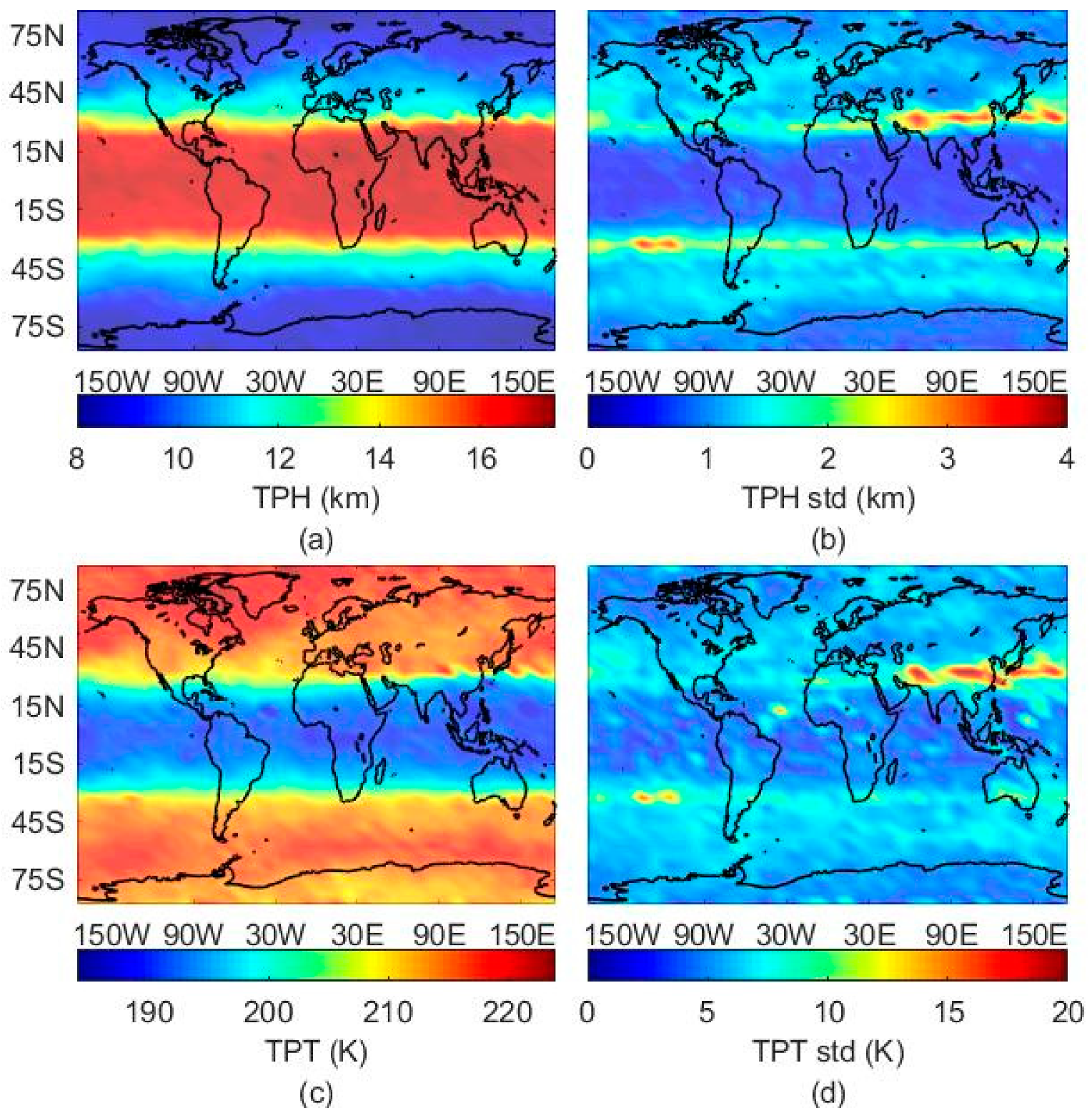
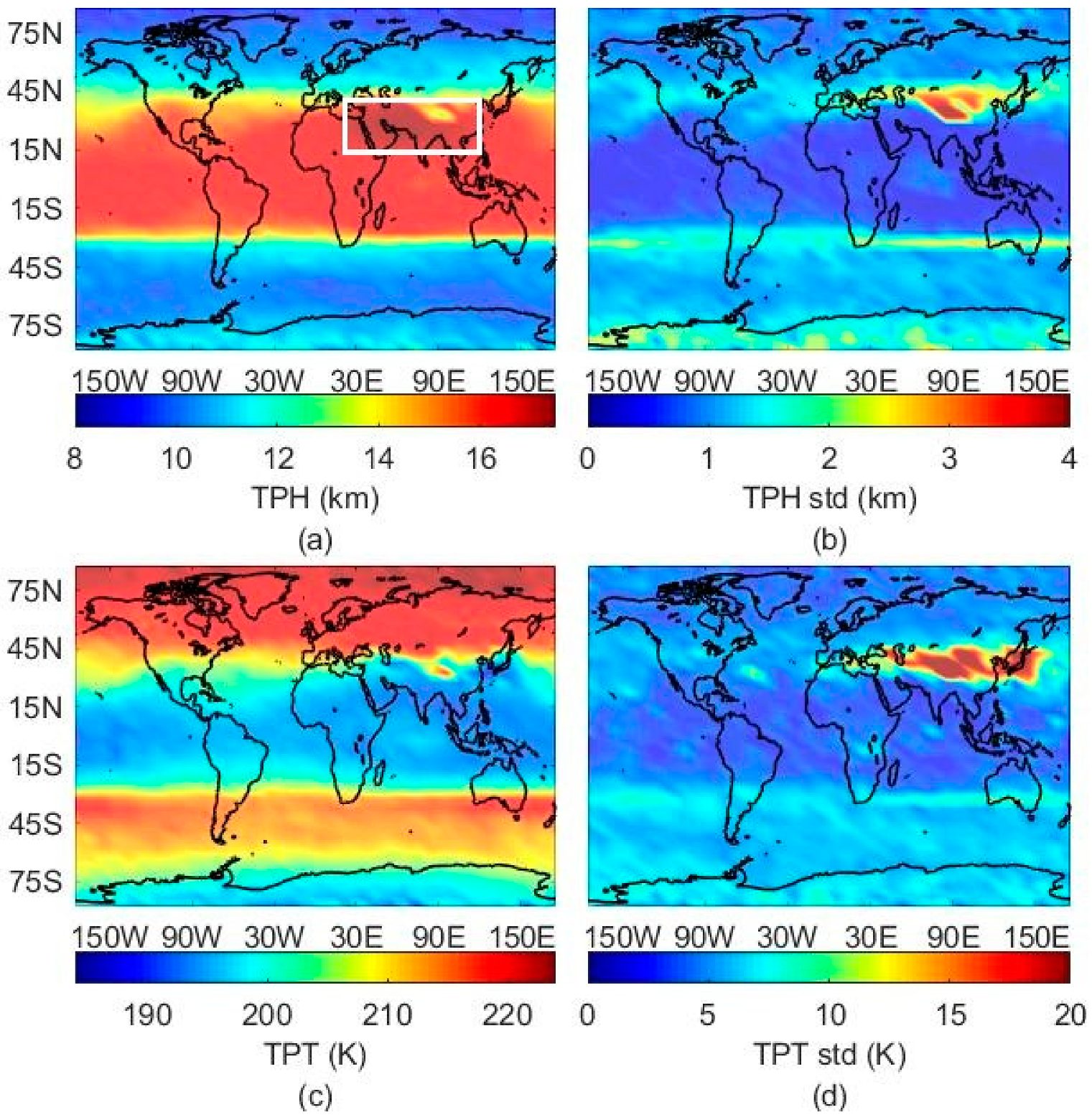
3.4. FY-3C Global Tropopause Patterns

Figure 9, Figure 10, Figure 11, Figure 12 and Figure 13 introduce the global mean seasonal TPH and TPT derived from 2014–2017 FY-3C data. In each figure, the top left graph is for the mean of global TPH, and the top right graph is for the mean of standard deviation of global TPH, and similarly, the bottom left graph and the bottom right are for the mean of global TPT and the standard deviation of global TPT, respectively. The global standard deviation of TPH and TPT were less than 1.5 km and 8 K, respectively, for the whole year except for at 30N latitude and 30S latitude where the tropopause height changed drastically (e.g., the widening and the constriction of tropic tropopause in summer and winter). In spring (MAM), the global tropopause parameters presented a good symmetry between Southern and Northern hemispheres. In summer (JJA), the tropical tropopause widened toward the north pole and the southern boundary of tropical tropopause narrowed. In South Asia, the extremely high tropopause caused by deep convective activity was found [33], which confirms with the results of Rieckh et al. [21] and Li et al. [22]. This phenomenon also leads to the considerable variability of the tropopause, which was reflected in the high values in standard deviation panels. The region with 1 km higher tropopause may not be clear in Figure 10, and thus to give a clear view, Figure 11 presents the summer tropical tropopause height, in which an obvious region with 1 km higher tropopause is shown. During summer and autumn (SON), TPT above Antarctica reached its minima in the annual cycle while TPT above the Arctic reached its maxima, which was caused by the differences in dynamical heating of the stratosphere according to Zängl and Hoinka [34]. Correspondingly, TPH above Antarctica rises obviously, about 2 km higher than it in spring, while TPH above the Arctic increased less than 1 km, which agrees with the results of Tomikawa et al. [35]. In winter (DJF), strong zonal asymmetry can be seen in the Northern hemisphere. TPH above the tropics increased to its maxima, and the corresponding TPT decreased to around 196 K. Similar to the results of Rieckh et al. [21] and Li et al. [22], two regions with extremely low TPH occured at Eastern Canada and Eastern Russia.

4. Discussion

The bias of temperature profiles between FY-3C and COSMIC is holistically less than 0.2 K except in the tropical region, where the mean temperature bias is prominent in the range of 5 km–7 km and 19 km and higher. The bias at 5 km–7 km is caused by the RO measuring error, for the high concentration of water vapor in lower troposphere, especially over tropics, which reduces the signal to noise ratio and may lead to complicated signal dynamics that cause tracking errors. Also, the bias gradually increases with height from 17 km only in the tropics. For this phenomenon, similar results can be seen in a study by Ladstädter et al. [36], who compared the temperature profiles between GPS RO data and radiosonde data, indicating that the temperature bias is 0.3 K at 17 km and gradually increases to higher than 1 K at 30 km. Even so, temperature profiles of two RO missions match well in the vicinity of the tropopause.
Compared with COSMIC tropopause parameters, FY-3C results show excellent coincidence in TPH, with the overall bias less than 100 m, which is the interpolation interval of temperature profiles. However, in 60N–90N, FY-3C mean TPH is more than 100 m lower in June, and in 60S–90S, FY-3C TPH is obviously higher (about 200 m) on August and September. TPH over the Arctic decreases to its lowest point in June and TPH over Antarctica rises to its highest point. The TPH AMD over the South pole during July to November is evidently large, and this may be because during this time, the Antarctic polar vortex reaches its highest strength, and this may lead to unrealistic TPH [22]. However, it seems that FY-3C TPH reflects a more sensitive TPH variation in high latitudes. On the other hand, the mean bias of TPT comparison is less than 1 K, but large bias occurs on January, February and March over the tropics and mid latitude regions in the Southern hemisphere.
For the tropopause parameters comparison between FY-3C and radiosonde, the average TPH bias is similar with that in comparison between FY-3C and COSMIC, and the average TPT bias is relatively less. However, SGP (36.4N, 96.2W) shows an obvious difference with FY-3C. It may be because SGP station is located at the latitude where the tropopause height changes abruptly with latitude compared with other regions (this can be seen in Figure 9, Figure 10, Figure 12 and Figure 13) and thus compared with other stations, 300 km distance may lead to larger error at SGP. Over all, the TPH AMD is slightly larger than the comparison results with COSMIC but the TPT AMD is smaller.
Several phenomena shown in tropopause global patterns derived from FY-3C data match well with the results of other relevant research that are mentioned in Section 3.4. The global TPT and TPH standard deviation are slightly larger than those in Li et al. [22] where seven RO missions from 2001 to 2013 were used. However, standard deviation is related to the amount of dates in each grid, for example, we chose a 5° × 10° grid, as we have mentioned above, and if we chose a 5° × 5° grid, the temperature standard deviation will increase to 15 K. Compared with the multi-mission data of 12 years, the amount of four years FY-3C data are quite small, and thus we believe this result points to good stability of FY-3C RO data in tropopause research.

5. Conclusions

The FY-3C GNOS mission was designed and developed by National Space Science Center, Chinese Academy of Sciences (NSSC, CAS), for sounding the Earth’s neutral atmosphere and ionosphere by using both the BDS and GPS signals. After five years data gathering, FY-3C atmosphere profiles are ready to be used in climate and atmospheric research. The variation of thermal tropopause is a hot topic in atmosphere and climate research, and thus we choose this topic as the first climate research subject based on FY-3C GNOS data to confirm the validity of FY-3C data in climate research. In this study, we validate the utility of FY-3C GNOS atmosphere data from January 2014 to December 2017 in tropopause research via the comparison with COSMIC data and radiosonde data, as well as results of other relevant studies.
In general, results from FY-3C show good agreement with results from COSMIC and radiosonde. The temperature mean difference and root mean square error between FY-3C and COSMIC are globally less than 0.2 K and 2 K, respectively, except for 18–22 km over the tropics, where FY-3C exhibits a less than 0.8 K positive bias and a 2–3 K root mean square error compared with temperature profiles of COSMIC. For the tropopause parameters, TPH and TPT, FY-3C has a positive bias of TPH of less than 100 m compared with COSMIC results, which meets the interpolation interval of temperature profiles, but the negative TPT bias is relatively large in several months, about 1–2 K. Likewise, FY-3C tropopause parameters are in accord with the radiosonde counterparts, with correlation coefficients larger than 0.9 and regression coefficients near 1 for the majority of chosen radiosonde stations in different latitudes in the Northern hemisphere.
The seasonal global tropopause patterns derived from FY-3C temperature profiles are discussed after the comparison with both undirect and direct atmosphere observing method. The global TPH standard deviation is about 0–1.5 km, and the global TPT standard deviation is about 0–8 K except for that in 30N latitude and 30S latitude, which shows the good stability of the FY-3C global tropopause parameter results. The clear appearance and disappearance of tropopause zonal asymmetry, the obvious temperature decrease of Antarctic tropopause and the extreme high and low tropopause are found, which coincide with the results of other relevant studies.
The above results demonstrate the utility of FY-3C GNOS atmosphere profiles in the research of the tropopause region, paving the way for the further atmosphere and climate research. FY-3C, as a sun-synchronous satellite, can provide global real-time time-concentrated observations, and we believe this will become a valuable data source for the development of climate applications and the promotion of the atmosphere and climate research. In the future, with the launch of following FY-3 series missions, the data density and the resolution will be improved, and FY-3 GNOS observations will be expected to provide an essential future contribution to the pool of international high-quality atmospheric RO products.

Author Contributions

Conceptualization, Z.L. and W.B.; Data curation, J.X., D.Z. and C.L.; Funding acquisition, Y.S., C.C., Q.D., X.W., X.M., Y.C. and D.W.; Resources, Y.S.; Software, Z.L., G.T. and Y.T.; Writing – original draft, Z.L.; Writing – review & editing, W.B.

Funding

This research was supported by the National Key R & D Program of China (Grant Nos. 2017YFB0502800 and 2017YFB0502802), the National Natural Science Foundation of China (Grant Nos. 41405040, 41775034, 41405039, 41505030 and 41606206), the Strategic Priority Research Program of Chinese Academy of Sciences (Grant No. XDA15007501), and the Scientific Research Project of the Chinese Academy of Sciences (Grant No. YZ201129).

Acknowledgments

We express our appreciation to CDAAC team for providing the COSMIC atmospheric data and National Oceanic and Atmospheric Administration (NOAA) for their GRUAN and IGRA radiosonde data.

Conflicts of Interest

The authors declare no conflict of interest.

References

  1. Holton, J.R.; Haynes, P.H.; Mcintyre, M.E.; Douglass, A.R.; Pfister, L. Stratosphere-troposphere exchange. Rev. Geophys. 1995, 33, 403–439. [Google Scholar] [CrossRef]
  2. Randel, W.J.; Wu, F.; Vömel, H.; Nedoluha, G.E.; Forster, P. Decreases in stratospheric water vapor after 2001: Links to changes in the tropical tropopause and the Brewer-Dobson circulation. J. Geophys. Res. 2006, 111. [Google Scholar] [CrossRef] [Green Version]
  3. Randel, W.J.; Wu, F.; Oltmans, S.J.; Rosenlof, K.; Nedoluha, G. Interannual changes of stratospheric water vapor and correlations with tropical tropopause temperatures. J. Atmos. Sci. 2004, 61, 2133–2148. [Google Scholar] [CrossRef]
  4. Fueglistaler, S.; Dessler, A.E.; Dunkerton, T.J.; Folkins, I.; Fu, Q.; Mote, P. Tropical tropopause layer. Rev. Geophys. 2009, 47. [Google Scholar] [CrossRef] [Green Version]
  5. Santer, B.D.; Wehne, M.F.; Wigley, T.M.L.; Sausen, R.; Meehl, G.A.; Taylor, K.E.; Ammann, C.; Arblaster, J.; Washington, W.M.; Boyle, J.S.; et al. Contributions of anthropogenic and natural forcing to recent tropopause height changes. Science 2003, 301, 479–483. [Google Scholar] [CrossRef] [PubMed]
  6. Lorenz, D.J.; DeWeaver, E.T. Tropopause height and zonal wind response to global warming in the IPCC scenario integrations. J. Geophys. Res. 2007, 112. [Google Scholar] [CrossRef] [Green Version]
  7. Steinbrecht, W.; Claude, H.; Köhler, U.; Hoinka, K.P. Correlations between Tropopause Height and Total Ozone: Implications for Long-Term Changes. J. Geophys. Res. 1998, 103, 19183–19192. [Google Scholar] [CrossRef]
  8. Sausen, R.; Santer, B.D. Use of changes in tropopause height to detect human influences on climate. Meteorol. Z. 2003, 12, 131–136. [Google Scholar] [CrossRef]
  9. Birner, T.; Sankey, D.; Shepherd, T.G. The tropopause inversion layer in models and analyses. Geophys. Res. Lett. 2006, 33. [Google Scholar] [CrossRef] [Green Version]
  10. Sturaro, G. A closer look at the climatological discontinuities present in the NCEP/NCAR reanalysis temperature due to the introduction of satellite data. Clim. Dyn. 2003, 21, 309–316. [Google Scholar] [CrossRef]
  11. Sterl, A. On the (in-)homogeneity of reanalysis products. J. Clim. 2004, 17, 3866–3873. [Google Scholar] [CrossRef]
  12. Biondi, R.; Steiner, A.K.; Kirchengast, G.; Rieckh, T. Characterization of thermal structure and conditions for overshooting of tropical and extratropical cyclones with GPS radio occultation. Atmos. Chem. Phys. 2015, 15, 5181–5193. [Google Scholar] [CrossRef] [Green Version]
  13. Ravindra Babu, S.; Venkat Ratnam, S.; Basha, G.; Krishnamurthy, B.V.; Venkateswararao, B. Effect of tropical cyclones on the tropical tropopause parameters observed using COSMIC GPS RO data. Atmos. Chem. Phys. 2015, 15, 10239–10249. [Google Scholar] [CrossRef] [Green Version]
  14. Nishida, M.; Shimizu, A.; Tsuda, T.; Rocken, C.; Ware, R.H. Seasonal and longitudinal variations in the tropical tropopause observed with the GPS occultation technique (GPS/MET). J. Meteorol. Soc. Jpn. 2000, 78, 691–700. [Google Scholar] [CrossRef]
  15. Randel, W.J.; Wu, F.; Rivera, R.W. Thermal variability of the tropical tropopause region derived from GPS/MET observations. J. Geophys. Res. Atmos. 2003, 108. [Google Scholar] [CrossRef]
  16. Schmidt, T.; Wickert, J.; Beyerle, G.; Reigber, C. Tropical tropopause parameters derived from GPS radio occultation measurements with CHAMP. J. Geophys. Res. Atmos. 2004, 109. [Google Scholar] [CrossRef] [Green Version]
  17. Schmidt, T.; Heise, S.; Wickert, J.; Beyerle, G.; Reigber, C. Gps radio occultation with champ and sac-c: Global monitoring of thermal tropopause parameters. Atmos. Chem. Phys. 2005, 5, 1473–1488. [Google Scholar] [CrossRef]
  18. Schmidt, T.; Wickert, J.; Beyerle, G.; Heise, S. Global tropopause height trends estimated from GPS radio occultation data. Geophys. Res. Lett. 2008, 35. [Google Scholar] [CrossRef] [Green Version]
  19. Kim, J.; Son, S.W. Tropical Cold-Point Tropopause: Climatology, Seasonal Cycle, and Intraseasonal Variability Derived from COSMIC GPS Radio Occultation Measurements. J. Clim. 2012, 25, 5343–5360. [Google Scholar] [CrossRef]
  20. Son, S.W.; Tandon, N.F.; Polvani, L.M. The fin-scale structure of the global tropopause derived from COSMIC GPS radio occultation measurements. J. Geophys. Res. 2011, 116. [Google Scholar] [CrossRef]
  21. Rieckh, T.; Scherllin-Pirscher, B.; Ladstädter, F.; Foelsche, U. Characteristics of tropopause parameters as observed with GPS radio occultation. Atmos. Meas. Tech. 2014, 7, 4693–4727. [Google Scholar] [CrossRef]
  22. Li, W.; Yuan, Y.B.; Chai, Y.J.; Liou, Y.A.; Ou, J.M.; Zhong, S.M. Characteristics of the global thermal tropopause derived from multiple radio occultation measurements. Atmos. Res. 2017, 185, 142–157. [Google Scholar] [CrossRef]
  23. Wang, X.Y.; Sun, Y.Q.; Du, Q.F.; Bai, W.H.; Wang, D.W.; Cai, Y.R.; Wu, D.; Yu, Q.L. GNOS—Radio Occultation Sounder on Board of Chinese FY3 Satellites. In Proceedings of the 2014 IEEE Geoscience and Remote Sensing Symposium (IGARSS 2014), Quebec, QC, Canada, 13–18 July 2014; pp. 4982–4985. [Google Scholar] [CrossRef]
  24. Sun, Y.Q.; Bai, W.H.; Liu, C.L.; Liu, Y.; Du, Q.F.; Wang, X.Y.; Yang, G.L.; Liao, M.; Yang, Z.D.; Zhang, X.X.; et al. The FengYun-3C radio occultation sounder GNOS: A review of the mission and its early results and science applications. Atmos. Meas. Tech. 2018, 11, 5797–5811. [Google Scholar] [CrossRef]
  25. Bai, W.H.; Sun, Y.Q.; Du, Q.F.; Yang, G.L.; Yang, Z.D.; Zhang, P.; Bi, Y.M.; Wang, X.Y.; Cheng, C.; Han, Y. An introduction to the FY3 GNOS instrument and mountain-top tests. Atmos. Meas. Tech. 2014, 7, 1817–1823. [Google Scholar] [CrossRef] [Green Version]
  26. Du, Q.F.; Sun, Y.Q.; Bai, W.H.; Wang, X.Y.; Wang, D.W.; Meng, X.G.; Cai, Y.R.; Liu, C.L.; Wu, D.; Wu, C.J.; et al. The Next Generation GNOS Instrument for FY-3 Meteorological Satellites. In Proceedings of the 2016 IEEE International Geoscience and Remote Sensing Symposium (IGARSS 2016), Beijing, China, 10–15 July 2016; pp. 381–383. [Google Scholar] [CrossRef]
  27. Wang, S.-Z.; Zhu, G.-W.; Bai, W.-H.; Liu, C.; Sun, Y.-Q.; Du, Q.-F.; Wang, X.-Y.; Meng, X.-G.; Yang, G.-L.; Yang, Z.-D.; et al. For the first time fengyun3 C satellite-global navigation satellite system occultation sounder achieved spaceborne Bei Dou system radio occultation. Acta Phys. Sin. 2015, 64. [Google Scholar] [CrossRef]
  28. Bai, W.H.; Liu, C.L.; Meng, X.G.; Sun, Y.Q.; Kirchengast, G.; Du, Q.F.; Wang, X.Y.; Yang, G.L.; Liao, M.; Yang, Z.D.; et al. Evaluation of atmospheric profiles derived from single- and zero-difference excess phase processing of BeiDou radio occultation data from the FY-3C GNOS mission. Atmos. Meas. Tech. 2018, 11, 819–833. [Google Scholar] [CrossRef] [Green Version]
  29. Scherllin-Pirscher, B.; Steiner, A.K.; Kirchengast, G.; Schwärz, M.; Leroy, S.S. The power of vertical geolocation of atmospheric profiles from GNSS radio occultation. J. Geophys. Res. Atmos. 2017, 122, 1595–1616. [Google Scholar] [CrossRef] [Green Version]
  30. Lewis, H.W. A robust method for tropopause altitude identification using GPS radio occultation data. Geophys. Res. Lett. 2009, 36. [Google Scholar] [CrossRef] [Green Version]
  31. Schmidt, T.; Wickert, J.; Haser, A. Variability of the upper troposphere and lower stratosphere observed with GPS radio occultation bending angles and temperatures. Adv. Space Res. 2010, 46, 150–161. [Google Scholar] [CrossRef]
  32. Randel, W.J.; Seidel, D.J. Interannual variability of the tropical tropopause derived from radiosonde data and NCEP reanalyses. J. Geophys. Res. 2000, 105, 15509–15523. [Google Scholar] [CrossRef] [Green Version]
  33. Highwood, E.J.; Hoskins, B.J. The tropical tropopause. Q. J. R. Meteorol. Soc. 1998, 124, 1579–1604. [Google Scholar] [CrossRef]
  34. Zängl, G.; Hoinka, K.P. The Tropopause in the Polar Regions. J. Clim. 2001, 14, 3117–3139. [Google Scholar] [CrossRef]
  35. Tomikawa, Y.; Nishimura, Y.; Yamanouchi, T. Characteristics of tropopause and tropopause inversion layer in the polar region. Sola 2009, 5, 141–144. [Google Scholar] [CrossRef]
  36. Ladstädter, F.; Steiner, A.K.; Schwärz, M.; Kirchengast, G. Climate intercomparison of GPS radio occultation, RS90/92 radiosondes and GRUAN from 2002 to 2013. Atmos. Meas. Tech. 2015, 8, 1819–1834. [Google Scholar] [CrossRef] [Green Version]
Figure 1. Latitudinal (a) and temporal (b) distribution of 4 years of FY-3C (blue dot) and COSMIC (red dot) temperature profiles.
Remotesensing 11 01139 g001
Figure 2. Radiosonde stations distribution, red dots representing GRUAN stations and blue dots representing IGRA stations.
Remotesensing 11 01139 g002
Figure 3. Mean temperature deviation between FengYun 3 series C satellite global navigation satellite system occultation sounder (FY-3C GNOS) and Constellation Observing System for Meteorology, Ionosphere and Climate (COSMIC) in different latitude bands, and the number noted at the top-left corner of each panel is the number of collocated pairs.
Remotesensing 11 01139 g003
Figure 4. Root mean square error between FY-3C GNOS and COSMIC in different latitude bands.
Remotesensing 11 01139 g004
Figure 5. Panel (a) indicates the annual cycle mean tropopause height (TPH) retrieved from four years of collocated FY-3C and COSMIC data. Dashed lines are for COSMIC results and solid lines are for FY-3C results. Panel (b) and panel (c) show the mean and absolute deviation.
Remotesensing 11 01139 g005
Figure 6. Annual cycle mean tropopause temperature (TPT) (a), TPT mean deviation (b) and TPT absolute deviation (c), which is similar to Figure 5.
Remotesensing 11 01139 g006
Figure 7. TPH comparison results of FY-3C and radiosonde data of nine stations. The x-axis (FY-3C TPH results) and y-axis (radiosonde TPH results) are symmetric and the correlation coefficient r and linear regression coefficient l are located at the top-left corner of each panel.
Remotesensing 11 01139 g007
Figure 8. TPT comparison results, which are similar to Figure 7.
Remotesensing 11 01139 g008
Figure 9. Seasonal patterns of TPT and TPH derived from January 2014-December 2017 FY-3C data. This is for spring (March, April, May). The (a) panel is global TPH pattern and the (b) panel is for the standard deviation of global TPH. Similarly, the (c) panel and the (d) panel are for global TPT pattern and TPT standard deviation, respectively.
Remotesensing 11 01139 g009
Figure 10. Seasonal patterns (ad) of TPT and TPH for summer (June, July, August). White box points out the region where the tropopause is extremely high.
Remotesensing 11 01139 g010
Figure 11. Seasonal pattern of tropical TPH for summer (June, July, August). White box is the same with that in Figure 10.
Remotesensing 11 01139 g011
Figure 12. Seasonal patterns (ad) of TPT and TPH for autumn (September, October, November).
Remotesensing 11 01139 g012
Figure 13. Seasonal patterns (ad) of TPT and TPH for winter (December, January, February). Two white circles identify two areas where the tropopause is obviously low.
Remotesensing 11 01139 g013
Table 1. Information of radiosonde stations.
Station NameOrganizationLocationTime SpanData Amount
BARGRUAN71.4N, 155.6W2014.1–2017.121815
GRAGRUAN39.0N, 27.4W2017.1–2017.12477
LINGRUAN52.2N, 15.2E2014.1–2017.124310
NYAGRUAN78.9N, 13.8E2014.1–2017.121219
SGPGRUAN36.4N, 96.2W2014.1–2017.123578
SODGRUAN67.2N, 26.7E2014.1–2017.121318
USM00072402IGRA37.9N, 75.5W2016.1–2017.121498
FMM00091413IGRA9.5N, 138.1E2016.1–2017.121445
RMM00091376IGRA7.1N, 171.4E2016.1–2017.121453
Table 2. The statistical comparison results of FY-3C and radiosonde data of nine stations.
StationLocationCollocate PairsTPH AMDTPH MDTPT AMDTPT MD
BAR71.4N, 155.6W360.42 km0.27 km2.01 K–1.43 K
GRA39.0N, 27.4W150.17 km0.05 km1.17 K–0.22 K
LIN52.2N, 15.2E1510.35 km0.07 km2.13 K–0.32 K
NYA78.9N, 13.8E840.36 km0.21 km1.91 K–0.85 K
SGP36.4N, 96.2W480.69 km0.40 km2.42 K–1.70 K
SOD67.2N, 26.7E490.40 km0.20 km1.99 K–0.20 K
USM37.9N, 75.5W460.41 km0.15 km2.15 K0.08 K
FMM9.5N, 138.1E270.22 km0.05 km1.16 K–0.13 K
RMM7.1N, 171.4E180.28 km0.02 km1.51 K

