Improved Estimation of the Intrinsic Dimension of a Hyperspectral Image Using Random Matrix Theory


Abstract
:
1. Introduction
2. Materials and Methods
2.1. Three Real Hyperspectral Scenes and Simulated Versions of Them
2.2. Relevant Random Matrix Theory and a Review of Id Estimators Which Use This Theory
2.2.1. Marchenko-Pastur Law
2.2.2. The Largest Noise Eigenvalue
2.2.3. The Difference between the Largest and Second Largest Noise Eigenvalues
2.3. Comparison of Different Id Estimators
2.3.1. ID Estimation When the Band Error Variances Are Known
2.3.2. ID Estimation When the Band Error Variances Are Equal
2.3.3. ID Estimation When the Band Error Variances Are Unequal
2.4. Combining the Best Preprocessing and Id Estimation Methods
2.5. Further Reducing the Bias in and
| Algorithm 1 Adjusted EID estimation algorithm |
|
3. Results
4. Discussion
4.1. Endmember Variability
4.2. Deterministic Errors
4.3. Spectrally Correlated Errors
4.4. Spatially Correlated Errors
4.5. Signal-Dependent Errors
4.6. Non-Linear Mixing
5. Summary and Conclusions
Funding
Acknowledgments
Conflicts of Interest
Abbreviations
| RMT | random matrix theory |
| ID | intrinsic dimension |
| EID | effective intrinsic dimension |
| MP | Marchenko-Pastur |
| MR | modified regression |
| PMR | positively modified regression |
| probability density function | |
| cdf | cumulative distribution function |
| MNF | minimum noise fraction |
References
- Harsanyi, J.; Farrand, W.; Chang, C.I. Determining the number and identity of spectral endmembers: an integrated approach using Neyman-Pearson eigen-thresholding and iterative constrained RMS error minimization. In Proceedings of the Thematic Conference on Geologic Remote Sensing, Pasadena, CA, USA, 8–11 February 1993; Environmental Research Institute of Michigan: Ann Arbor, MI, USA, 1993; Volume 1, p. 395. [Google Scholar]
- Chang, C.I.; Du, Q. Estimation of number of spectrally distinct signal sources in hyperspectral imagery. IEEE Trans. Geosci. Remote Sens. 2004, 42, 608–619. [Google Scholar] [CrossRef]
- Kuybeda, O.; Malah, D.; Barzohar, M. Rank estimation and redundancy reduction of high-dimensional noisy signals with preservation of rare vectors. IEEE Trans. Signal Process. 2007, 55, 5579–5592. [Google Scholar] [CrossRef]
- Bioucas-Dias, J.; Nascimento, J. Hyperspectral subspace identification. IEEE Trans. Geosci. Remote Sens. 2008, 46, 2435–2445. [Google Scholar]
- Acito, N.; Diani, M.; Corsini, G. A new algorithm for robust estimation of the signal subspace in hyperspectral images in the presence of rare signal components. IEEE Trans. Geosci. Remote Sens. 2009, 47, 3844–3856. [Google Scholar]
- Eches, O.; Dobigeon, N.; Tourneret, J.Y. Estimating the number of endmembers in hyperspectral images using the normal compositional model and a hierarchical Bayesian algorithm. IEEE J. Sel. Top. Appl. Earth Obs. Remote Sens. 2010, 4, 582–591. [Google Scholar] [CrossRef]
- Bioucas-Dias, J.; Plaza, A.; Dobigeon, N.; Parente, M.; Du, Q.; Gader, P.; Chanussot, J. Hyperspectral unmixing overview: Geometrical, statistical and sparse regression-based approaches. IEEE J. Sel. Top. Appl. Earth Obs. Remote Sens. 2012, 5, 354–379. [Google Scholar] [CrossRef]
- Ambikapathi, A.; Chan, T.H.; Chi, C.Y.; Keizer, K. Hyperspectral data geometry-based estimation of number of endmembers using p-norm-based pure pixel identification algorithm. IEEE Trans. Geosci. Remote Sens. 2013, 51, 2753–2769. [Google Scholar] [CrossRef]
- Luo, B.; Chanussot, J.; Douté, S.; Zhang, L. Empirical automatic estimation of the number of endmembers in hyperspectral images. IEEE Geosci. Remote Sens. Lett. 2013, 10, 24–28. [Google Scholar]
- Bioucas-Dias, J.; Nascimento, J. Estimation of signal subspace on hyperspectral data. SPIE Proc. 2005, 5982, 191–198. [Google Scholar]
- Cawse-Nicholson, K.; Damelin, S.; Robin, A.; Sears, M. Determining the intrinsic dimension of a hyperspectral image using random matrix theory. IEEE Trans. Image Process. 2013, 22, 1301–1310. [Google Scholar] [CrossRef]
- Kritchman, S.; Nadler, B. Non-parametric detection of the number of signals: Hypothesis testing and random matrix theory. IEEE Trans. Signal Process. 2009, 57, 3930–3941. [Google Scholar] [CrossRef]
- Passemier, D.; Yao, J.F. On determining the number of spikes in a high-dimensional spiked population model. Random Matrices Theory Appl. 2012, 1, 1150002. [Google Scholar] [CrossRef]
- Halimi, A.; Honeine, P.; Kharouf, M.; Richard, C.; Tourneret, J.Y. Estimating the intrinsic dimension of hyperspectral images using a noise-whitened eigengap approach. IEEE Trans. Geosci. Remote Sens. 2016, 54, 3811–3821. [Google Scholar] [CrossRef]
- Berman, M.; Bischof, L.; Lagerstrom, R.; Guo, Y.; Huntington, J.; Mason, P.; Green, A.A. A comparison between three sparse unmixing algorithms using a large library of shortwave infrared mineral spectra. IEEE Trans. Geosci. Remote Sens. 2017, 55, 3588–3610. [Google Scholar] [CrossRef]
- Craig, M. Minimum-Volume Transforms for Remotely Sensed Data. IEEE Trans. Geosci. Remote Sens. 1994, 32, 542–552. [Google Scholar] [CrossRef]
- Winter, M.E. N-FINDR: An algorithm for fast autonomous spectral end-member determination in hyperspectral data. In Proceedings of the SPIE’s International Symposium on Optical Science, Engineering, and Instrumentation, Denver, CO, USA, 18–23 July 1999; pp. 266–275. [Google Scholar]
- Berman, M.; Kiiveri, H.; Lagerstrom, R.; Ernst, A.; Dunne, R.; Huntington, J. ICE: A statistical approach to identifying endmembers. IEEE Trans. Geosci. Remote Sens. 2004, 42, 2085–2095. [Google Scholar] [CrossRef]
- Nascimento, J.M.P.; Bioucas-Dias, J. Vertex component analysis: A fast algorithm to unmix hyperspectral data. IEEE Trans. Geosci. Remote Sens. 2005, 43, 898–910. [Google Scholar] [CrossRef]
- Miao, L.; Qi, H. Endmember extraction from highly mixed data using minimum volume constrained nonnegative matrix factorization. IEEE Trans. Geosci. Remote Sens. 2007, 45, 765–777. [Google Scholar] [CrossRef]
- Hao, Z.; Berman, M.; Guo, Y.; Stone, G.; Johnstone, I. Semi-realistic simulations of natural hyperspectral scenes. IEEE J. Sel. Top. Appl. Earth Obs. Remote Sens. 2016, 9, 4407–4419. [Google Scholar] [CrossRef]
- Berman, M.; Hao, Z.; Stone, G.; Guo, Y. An investigation into the impact of band error variance estimation on intrinsic dimension estimation in hyperspectral images. IEEE J. Sel. Top. Appl. Earth Obs. Remote Sens. 2018, 11, 3279–3296. [Google Scholar] [CrossRef]
- Green, R.O.; Eastwood, M.L.; Sarture, C.M.; Chrien, T.G.; Aronsson, M.; Chippendale, B.J.; Faust, J.A.; Pavri, B.E.; Chovit, C.J.; Solis, M.; et al. Imaging spectroscopy and the Airborne Visible/Infrared Imaging Spectrometer (AVIRIS). Remote Sens. Environ. 1998, 65, 227–248. [Google Scholar] [CrossRef]
- Cocks, T.; Jenssen, R.; Stewart, A.; Wilson, I.; Shields, T. The HyMap airborne hyperspectral sensor: The system, calibration and performance. In Proceedings of the 1st EARSeL Workshop on Imaging Spectroscopy, Zurich, Switzerland, 6–8 October 1998; Schaepman, M., Schlapfer, D., Itten, K., Eds.; EARSeL: Paris, France, 1998; pp. 37–42. [Google Scholar]
- Roger, R. Principal Components transform with simple automatic noise adjustment. Int. J. Remote Sens. 1996, 17, 2719–2727. [Google Scholar] [CrossRef]
- Mahmood, A.; Robin, A.; Sears, M. Modified residual method for the estimation of noise in hyperspectral images. IEEE Trans. Geosci. Remote Sens. 2017, 55, 1451–1460. [Google Scholar] [CrossRef]
- Gao, L.; Du, Q.; Zhang, B.; Yang, W.; Wu, Y. A comparative study on linear regression-based noise estimation for hyperspectral imagery. IEEE J. Sel. Top. Appl. Earth Obs. Remote Sens. 2013, 6, 488–498. [Google Scholar] [CrossRef]
- Robin, A.; Cawse-Nicholson, K.; Mahmood, A.; Sears, M. Estimation of the intrinsic dimension of hyperspectral images: Comparison of current methods. IEEE J. Sel. Top. Appl. Earth Obs. Remote Sens. 2015, 8, 2854–2861. [Google Scholar] [CrossRef]
- Meyer, T.R.; Drumetz, L.; Chanussot, J.; Bertozzi, A.L.; Jutten, C. Hyperspectral unmixing with material variability using social sparsity. In Proceedings of the 2016 IEEE International Conference on Image Processing (ICIP), Phoenix, AZ, USA, 25–28 September 2016; pp. 2187–2191. [Google Scholar]
- Zhou, Y.; Wetherley, E.B.; Gader, P.D. Unmixing urban hyperspectral imagery with a Gaussian mixture model on endmember variability. arXiv 2018, arXiv:1801.08513. [Google Scholar]
- Marchenko, V.A.; Pastur, L.A. Distribution of eigenvalues for some sets of random matrices. Mat. Sb. 1967, 114, 507–536. [Google Scholar]
- Baik, J.; Silverstein, J.W. Eigenvalues of large sample covariance matrices of spiked population models. J. Multivar. Anal. 2006, 97, 1382–1408. [Google Scholar] [CrossRef]
- Geman, S. A limit theorem for the norm of random matrices. Ann. Probab. 1980, 8, 252–261. [Google Scholar] [CrossRef]
- Johnstone, I.M. On the distribution of the largest eigenvalue in principal components analysis. Ann. Stat. 2001, 29, 295–327. [Google Scholar] [CrossRef]
- Roy, S.N. On a heuristic method of test construction and its use in multivariate analysis. Ann. Math. Stat. 1953, 24, 220–238. [Google Scholar] [CrossRef]
- Wax, M.; Kailath, T. Detection of signals by information theoretic criteria. IEEE Trans. Acoust. Speech Signal Process. 1985, 33, 387–392. [Google Scholar] [CrossRef]
- Meer, P.; Jolion, J.M.; Rosenfeld, A. A fast parallel algorithm for blind estimation of noise variance. IEEE Trans. Pattern Anal. Mach. Intell. 1990, 12, 216–223. [Google Scholar] [CrossRef]
- Clark, R.N.; Swayze, G.A.; Livo, K.E.; Kokaly, R.F.; Sutley, S.J.; Dalton, J.B.; McDougal, R.R.; Gent, C.A. Earth and planetary remote sensing with the USGS Tetracorder and expert systems. J. Geophys. Res. 2003, 83, 5131–5175. [Google Scholar]
- Bateson, C.A.; Asner, G.P.; Wessman, C.A. Endmember bundles: A new approach to incorporating endmember variability into spectral mixture analysis. IEEE Trans. Geosci. Remote Sens. 2000, 38, 1083–1094. [Google Scholar] [CrossRef]
- Somers, B.; Asner, G.P.; Tits, L.; Coppin, P. Endmember variability in spectral mixture analysis: A review. Remote Sens. Environ. 2011, 115, 1603–1616. [Google Scholar] [CrossRef]
- Zare, A.; Ho, K. Endmember variability in hyperspectral analysis: Addressing spectral variability during spectral unmixing. IEEE Signal Process. Mag. 2014, 31, 95–104. [Google Scholar] [CrossRef]
- Green, A.; Berman, M.; Switzer, P.; Craig, M. A transformation for ordering multispectral data in terms of image quality with implications for noise removal. IEEE Trans. Geosci. Remote Sens. 1988, 26, 65–74. [Google Scholar] [CrossRef]
- Ponomarenko, N.N.; Lukin, V.V.; Egiazarian, K.O.; Astola, J.T. A method for blind estimation of spatially correlated noise characteristics. In Image Processing: Algorithms and Systems VIII; International Society for Optics and Photonics: Bellingham, WA, USA, 2010; Volume 7532, p. 753208. [Google Scholar]
- Abramova, V.; Abramov, S.; Lukin, V.; Roenko, A.; Vozel, B. Automatic estimation of spatially correlated noise variance in spectral domain for images. Telecommun. Radio Eng. 2014, 73, 511–527. [Google Scholar] [CrossRef]
- Acito, N.; Diani, M.; Corsini, G. Signal-dependent noise modeling and model parameter estimation in hyperspectral images. IEEE Trans. Geosci. Remote Sens. 2011, 49, 2957–2971. [Google Scholar] [CrossRef]
- Meola, J.; Eismann, M.T.; Moses, R.L.; Ash, J.N. Modeling and estimation of signal-dependent noise in hyperspectral imagery. Appl. Opt. 2011, 50, 3829–3846. [Google Scholar] [CrossRef]
- Uss, M.L.; Vozel, B.; Lukin, V.V.; Chehdi, K. Local signal-dependent noise variance estimation from hyperspectral textural images. IEEE J. Sel. Top. Appl. Earth Obs. Remote Sens. 2011, 5, 469–486. [Google Scholar] [CrossRef]
- Somers, B.; Cools, K.; Delalieux, S.; Stuckens, J.; Van der Zande, D.; Verstraeten, W.W.; Coppin, P. Nonlinear hyperspectral mixture analysis for tree cover estimates in orchards. Remote Sens. Environ. 2009, 113, 1183–1193. [Google Scholar] [CrossRef]
- Halimi, A.; Altmann, Y.; Dobigeon, N.; Tourneret, J.Y. Nonlinear unmixing of hyperspectral images using a generalized bilinear model. IEEE Trans. Geosci. Remote Sens. 2011, 49, 4153–4162. [Google Scholar] [CrossRef]
- Altmann, Y.; Halimi, A.; Dobigeon, N.; Tourneret, J.Y. Supervised nonlinear spectral unmixing using a postnonlinear mixing model for hyperspectral imagery. IEEE Trans. Image Process. 2012, 21, 3017–3025. [Google Scholar] [CrossRef]
- Chen, J.; Richard, C.; Honeine, P. Nonlinear unmixing of hyperspectral data based on a linear-mixture/nonlinear-fluctuation model. IEEE Trans. Signal Process. 2013, 61, 480–492. [Google Scholar] [CrossRef]
- Dobigeon, N.; Tourneret, J.Y.; Richard, C.; Bermudez, J.C.M.; McLaughlin, S.; Hero, A.O. Nonlinear unmixing of hyperspectral images: Models and algorithms. IEEE Signal Process. Mag. 2014, 31, 82–94. [Google Scholar] [CrossRef]
- Heylen, R.; Parente, M.; Gader, P. A review of nonlinear hyperspectral unmixing methods. IEEE J. Sel. Top. Appl. Earth Obs. Remote Sens. 2014, 7, 1844–1868. [Google Scholar] [CrossRef]


| Scene | d | N |
|---|---|---|
| Indian Pines | 193 | 21,025 |
| Cuprite | 185 | 314,368 |
| Mt. Isa | 124 | 294,460 |
| Scene | ID | EID | |
|---|---|---|---|
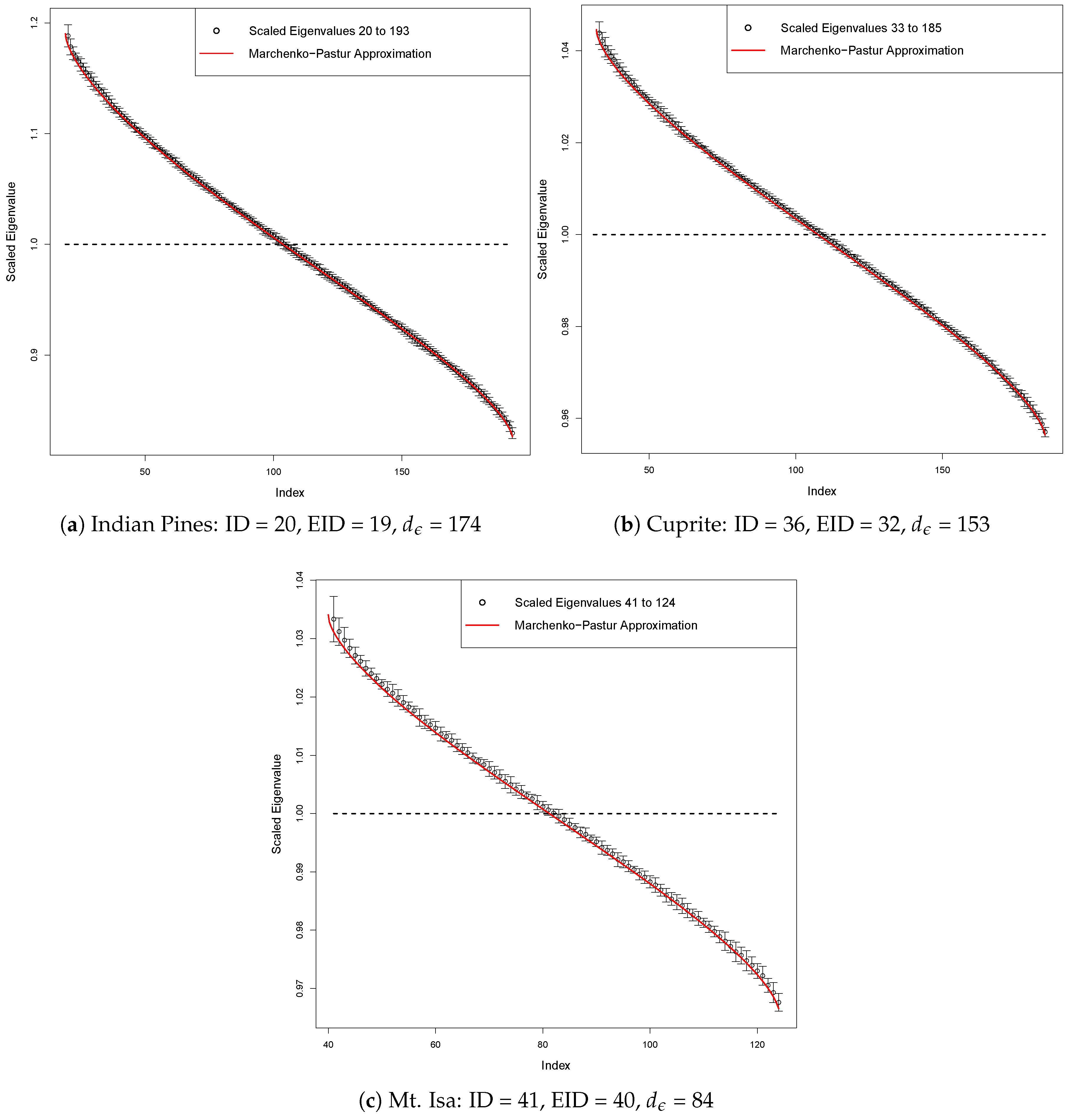
| Indian Pines | 20 | 19 | 174 |
| Cuprite | 36 | 32 | 153 |
| Mt. Isa | 41 | 40 | 84 |
| Estimator | Indian Pines | Cuprite | Mt. Isa |
|---|---|---|---|
| 11 | 16 | 17 | |
| 19, 19, 18 | 29, 28, 24 | 32, 27, 25 | |
| 20 | 33 | 61 | |
| 24 | 180 | 119 | |
| 24 | 39 | 56 | |
| 56 | 46 | 65 | |
| 54 | 46 | 65 | |
| Adj. | 53, 52, 52 | 46, 48, 48 | 65, 65, 65 |
| Adj. | 49, 46, 46 | 45, 47, 48 | 63, 63, 63 |
© 2019 by the author. Licensee MDPI, Basel, Switzerland. This article is an open access article distributed under the terms and conditions of the Creative Commons Attribution (CC BY) license (http://creativecommons.org/licenses/by/4.0/).
Share and Cite
Berman, M. Improved Estimation of the Intrinsic Dimension of a Hyperspectral Image Using Random Matrix Theory. Remote Sens. 2019, 11, 1049. https://doi.org/10.3390/rs11091049
Berman M. Improved Estimation of the Intrinsic Dimension of a Hyperspectral Image Using Random Matrix Theory. Remote Sensing. 2019; 11(9):1049. https://doi.org/10.3390/rs11091049
Chicago/Turabian StyleBerman, Mark. 2019. "Improved Estimation of the Intrinsic Dimension of a Hyperspectral Image Using Random Matrix Theory" Remote Sensing 11, no. 9: 1049. https://doi.org/10.3390/rs11091049
APA StyleBerman, M. (2019). Improved Estimation of the Intrinsic Dimension of a Hyperspectral Image Using Random Matrix Theory. Remote Sensing, 11(9), 1049. https://doi.org/10.3390/rs11091049