Estimation of Changes of Forest Structural Attributes at Three Different Spatial Aggregation Levels in Northern California using Multitemporal LiDAR

 , ,
, , 
Abstract
1. Introduction
2. Materials and Methods
2.1. Study Area
2.2. Sampling Design and Field Data
2.3. LiDAR Data Acquisitions
2.4. AOIs, Target Parameter and Overview of Modelling Strategies
2.5. -Modeling Method
2.5.1. Model -modeling Method
2.5.2. Target Parameter -modeling Method
2.5.3. Model Selection and Estimator -modeling Method
2.5.4. MSE Estimators for the -modeling Method
2.6. -Modeling Method
2.6.1. Model -modeling Method
2.6.2. Target Parameter -modeling Method
2.6.3. Estimator -modeling Method, and Estimator of the MSE
2.7. Comparison of Methods
2.7.1. General Accuracy Assessment
2.7.2. AOI-specific Comparisons.
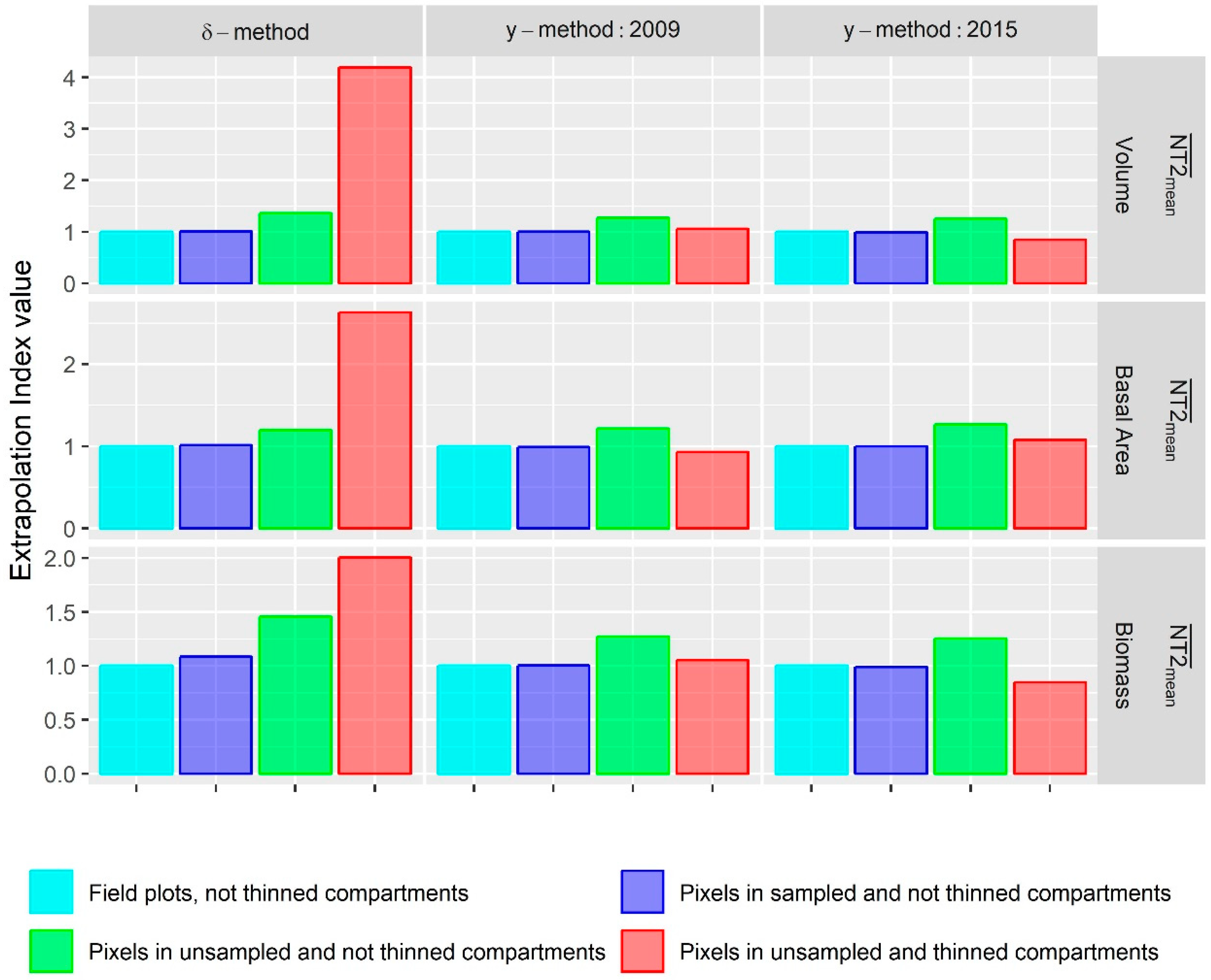
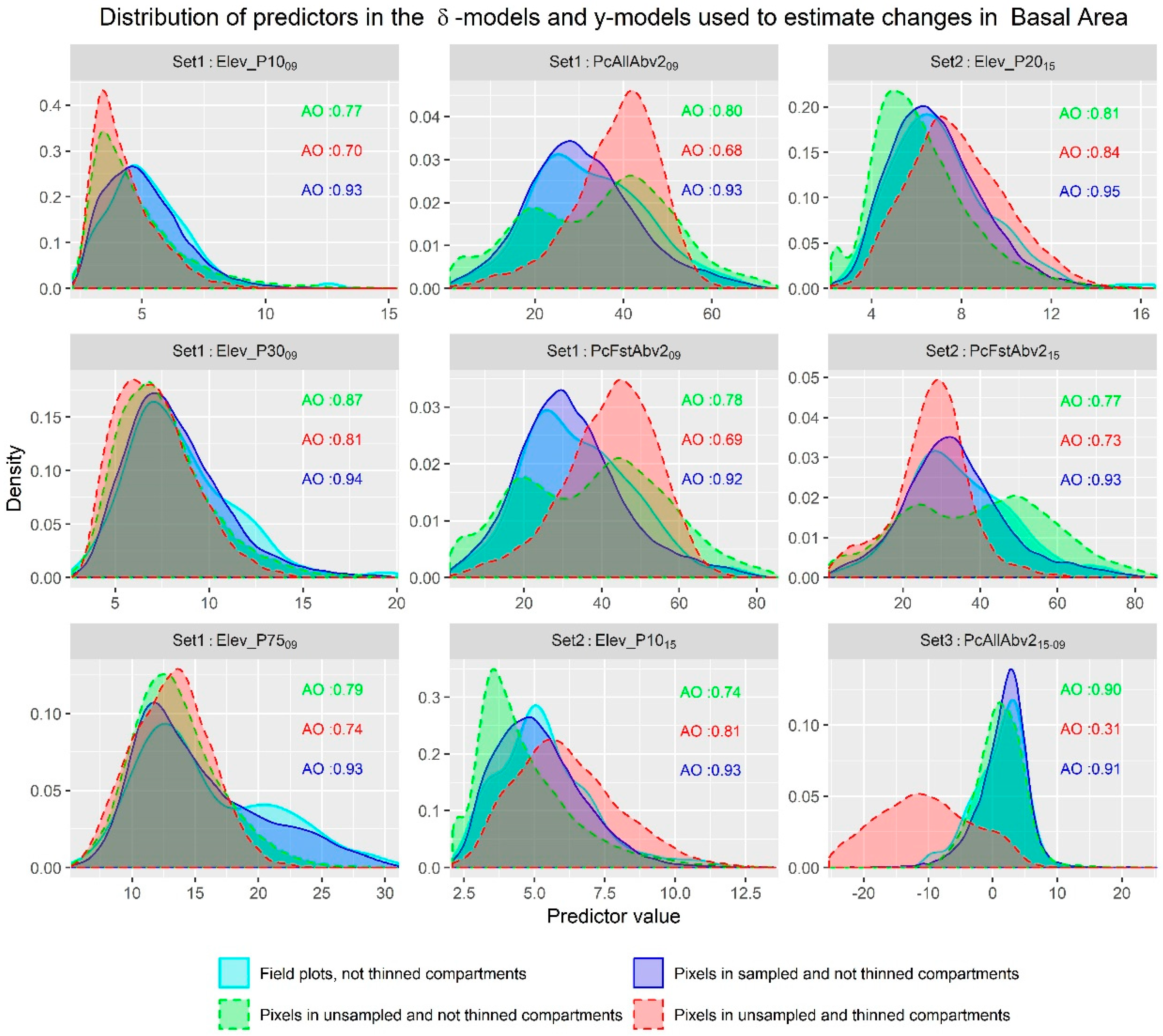
2.7.3. Extrapolation to Thinned Stands
3. Results
3.1. Selected Models -modeling Method and -modeling Method
3.2. General Accuracy Assessment and Comparison of Methods
3.3. AOI-Specific Estimates
3.3.1. Entire Study Area
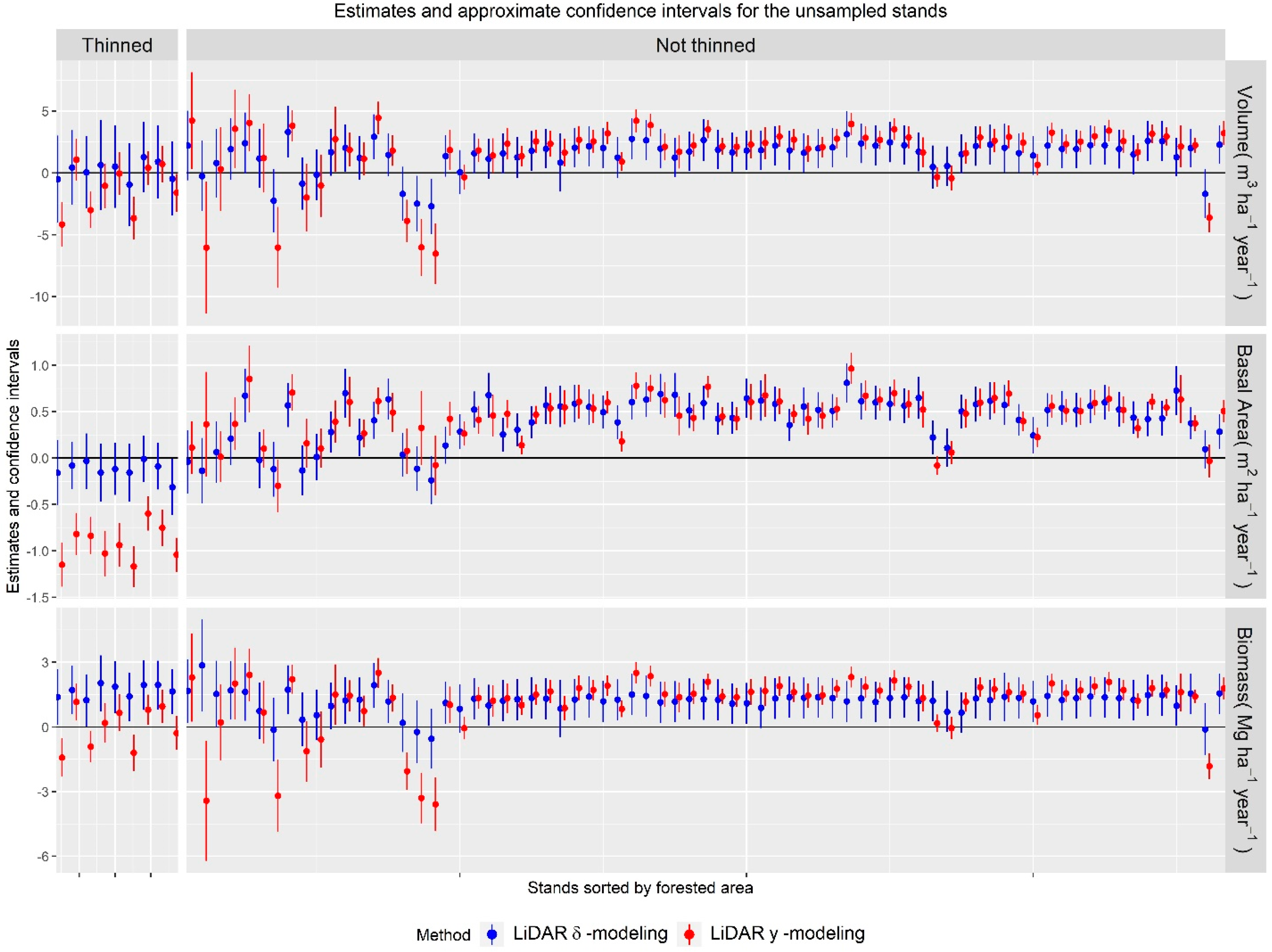
3.3.2. Stands
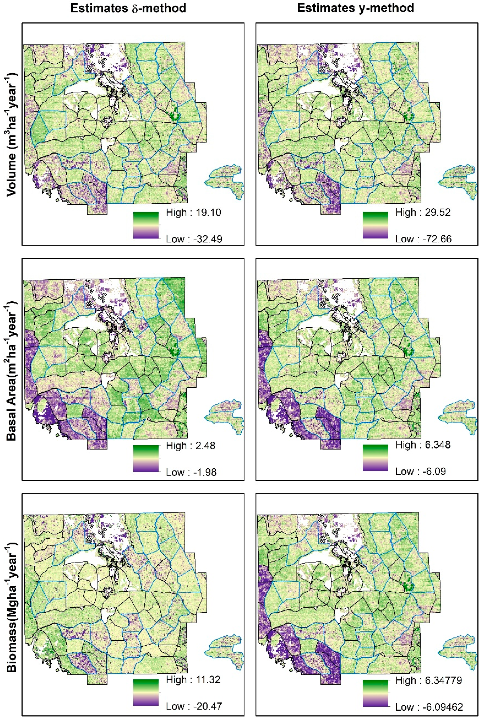
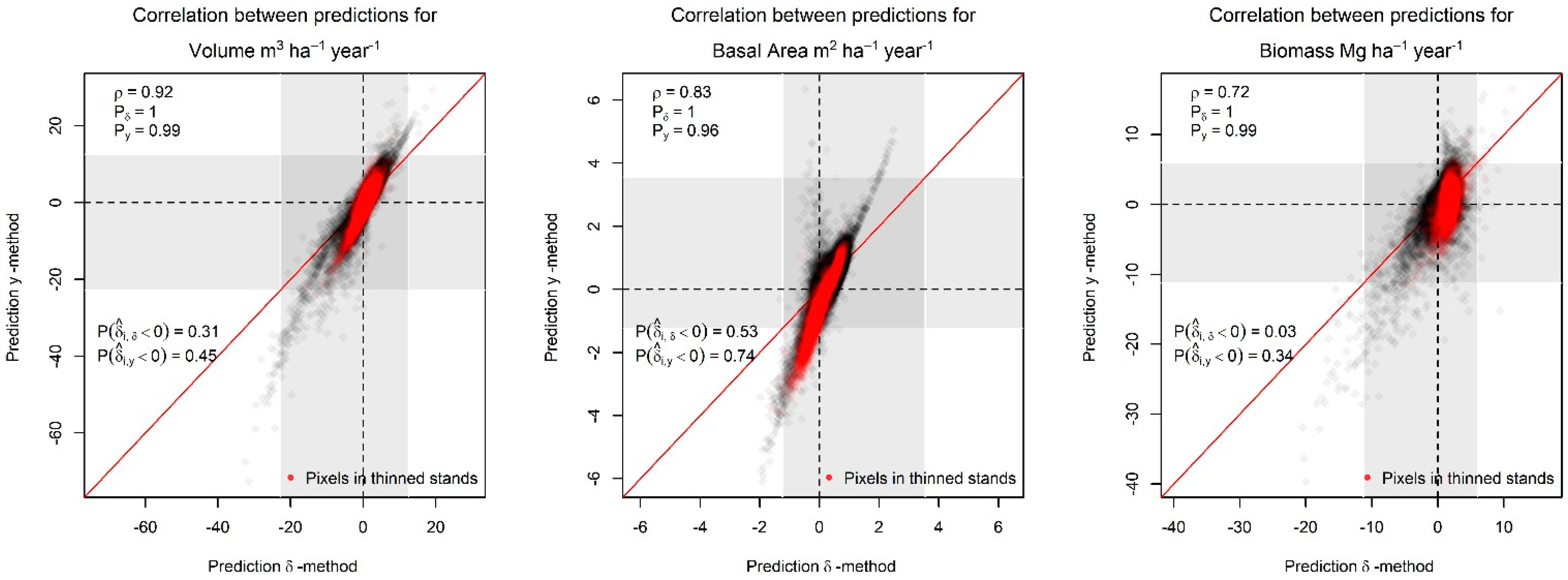
3.3.3. Pixel-level
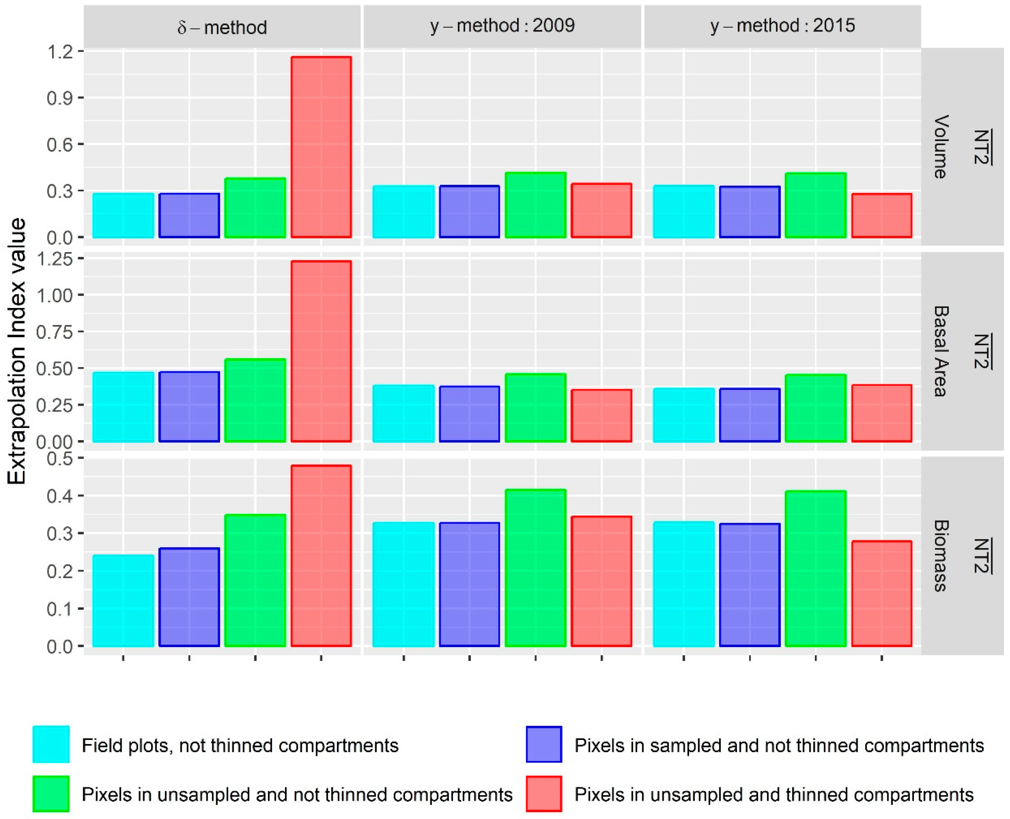
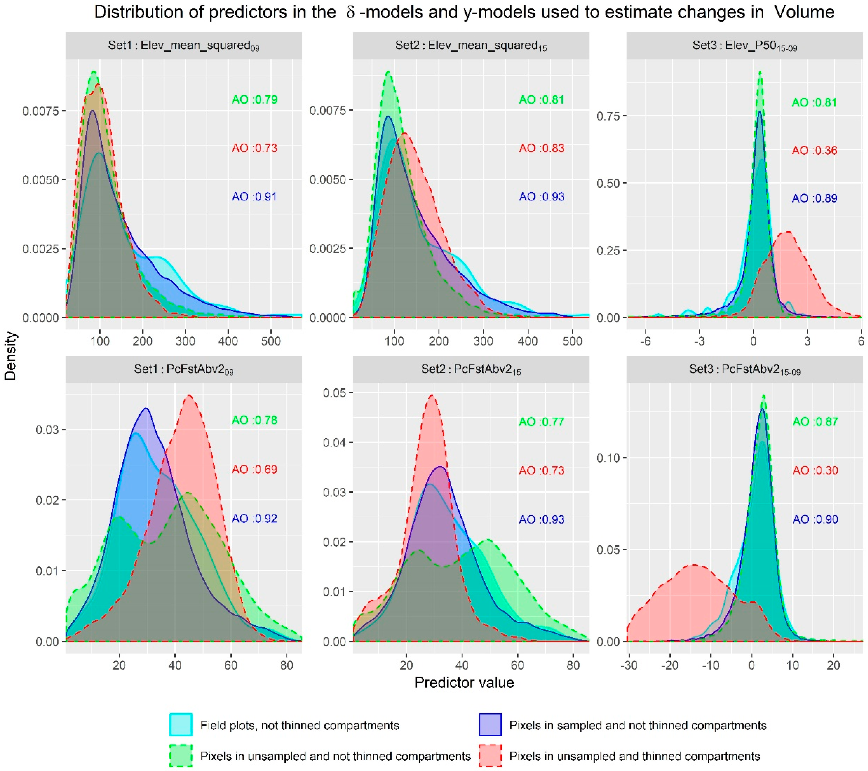
3.4. Extrapolation to Thinned Stands
4. Discusion
4.1. General Accuracy Assessment and Comparison of Methods.
4.2. AOI-Specific Estimates
4.2.1. Entire Study Area
4.2.2. Stands
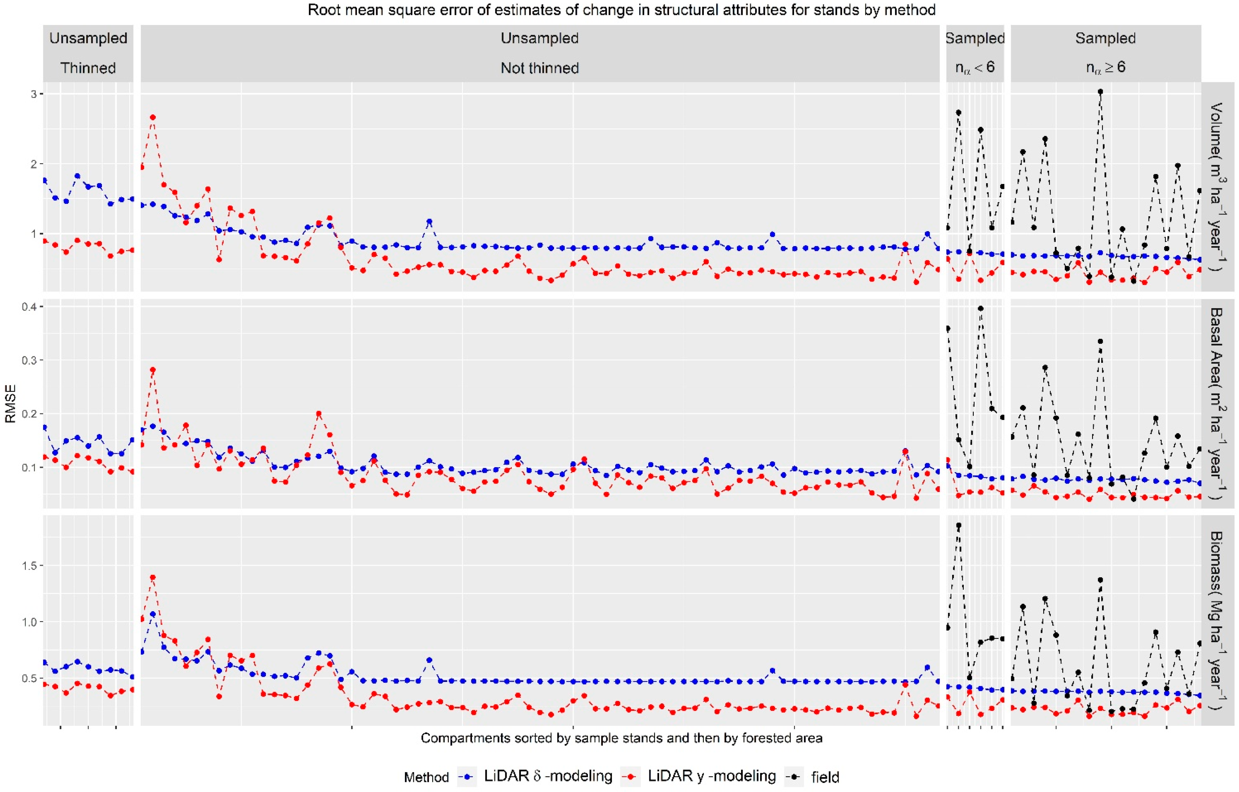
4.2.3. Pixel-level
4.3. Advantages of Modeling Alternatives
5. Conclusions
- The change of structural attributes and LiDAR auxiliary information are weakly correlated. This weak correlation seems to more evident in BMEF than in previous studies because of the slower growth in the study area and the relatively short lapse of time between LiDAR acquisitions, which indicates that for future studies in similar areas it might be necessary to increase the time lags between LiDAR flights.
- In general, the -modeling method was found to be a slightly more accurate alternative to obtain estimates of change for the whole study area; however, the -modeling method was able to produce better estimates at the stand level. In addition, the -modeling method method also seemed to be less prone to extrapolation problems. This indicates that field campaigns for the -modeling method have to be carefully designed while the -modeling method might be less sensitive to certain bias problems.
- Despite the weak correlations with the changes in structural attributes, LiDAR auxiliary information allows obtaining estimates of growth for stands that improve over those derived using only field information.
- The large uncertainty observed for pixel-level predictions indicated that high-resolution maps of growth, generated using LiDAR auxiliary information in similar conditions, should be taken as approximated products.
Author Contributions
Funding
Acknowledgments
Conflicts of Interest
Appendix A

| Description Auxiliary Variables Sets 1, 2 and 3 | Acronym | Description Auxiliary Variables Set 4 | Acronym | ||
|---|---|---|---|---|---|
| Set 1 Year: 2009 | Set 2 Year: 2015 | Set 3, Difference 2015-2009 | Set 4 | ||
| Minimum, maximum, mean, mode, standard deviation, variance, coefficient of variation and interquartile range of the distribution of heights of the point cloud. | Elev_min09 | Elev_min15 | Elev_min15-09 | Incoming solar radiation | Solar_radiation |
| Elev_max09 | Elev_max15 | Elev_max15-09 | |||
| Elev_mean09 | Elev_mean15 | Elev_mean15-09 | Structural diversity, factor with three levels HiD, LoD and RNA. Coded using two dummy variables. RNA reference level. | HiD | |
| Elev_mean209 | Elev_mean215 | Elev_mean215-09 | |||
| Elev_mode09 | Elev_mode15 | Elev_mode15-09 | |||
| Elev_stddv09 | Elev_stddv15 | Elev_stddv15-09 | LoD | ||
| Elev_var09 | Elev_var15 | Elev_var15-09 | |||
| Elev_CV09 | Elev_CV15 | Elev_CV15-09 | Presence absence of prescribed fires. Coded using a dummy variable taking value 1 for stands where prescribed fires are applied and 0 otherwise. | Burned | |
| Elev_IQ09 | Elev_IQ15 | Elev_IQ15-09 | |||
| Elev_AAD09 | Elev_AAD15 | Elev_AAD15-09 | |||
| Elev_MADmed09 | Elev_MADmed15 | Elev_MADmed15-09 | |||
| Elev_MADmod09 | Elev_MADmod15 | Elev_MADmod15-09 | |||
| Percentiles of the distribution of heights of the point cloud. | Elev_P0109 | Elev_P0115 | Elev_P0115-09 | ||
| Elev_P0509 | Elev_P0515 | Elev_P0515-09 | |||
| Elev_P1009 | Elev_P1015 | Elev_P1015-09 | |||
| Elev_P2009 | Elev_P2015 | Elev_P2015-09 | |||
| Elev_P3009 | Elev_P3015 | Elev_P3015-09 | |||
| Elev_P4009 | Elev_P4015 | Elev_P4015-09 | |||
| Elev_P5009 | Elev_P5015 | Elev_P5015-09 | |||
| Elev_P6009 | Elev_P6015 | Elev_P6015-09 | |||
| Elev_P7009 | Elev_P7015 | Elev_P7015-09 | |||
| Elev_P7509 | Elev_P7515 | Elev_P7515-09 | |||
| Elev_P8009 | Elev_P8015 | Elev_P8015-09 | |||
| Elev_P9009 | Elev_P9015 | Elev_P9015-09 | |||
| Elev_P9509 | Elev_P9515 | Elev_P9515-09 | |||
| Elev_P9909 | Elev_P9915 | Elev_P9915-09 | |||
| Canopy relief ratio | CRR09 | CRR15 | CRR15-09 | ||
| Percentage of first (Fst) and all (All) returns above 2 m | PcFstAbv209 | PcFstAbv215 | PcFstAbv215-09 | ||
| PcAllAbv209 | PcAllAbv215 | PcAllAbv215-09 | |||
| Ratio all returns above 2 m to first returns | AllAbv2Fst09 | AllAbv2Fst15 | AllAbv2Fst15-09 | ||
| Percentage of first returns above the mean and mode | PcFstAbvMean09 | PcFstAbvMean15 | PcFstAbvMean15-09 | ||
| PcFstAbvMode09 | PcFstAbvMode15 | PcFstAbvMode15-09 | |||
| Percentage of all returns above the mean and mode | PcAllAbvMean09 | PcAllAbvMean15 | PcAllAbvMean15-09 | ||
| PcAllAbvMode09 | PcAllAbvMode15 | PcAllAbvMode15-09 | |||
| Ratio of all returns above the mean and mode to number of first returns | AllAbvMeanFst09 | AllAbvMeanFst15 | AllAbvMeanFst15-09 | ||
| AllAbvModeFst09 | AllAbvModeFst15 | AllAbvModeFst15-09 | |||
| Proportion of points in the height intervals [0,0.5), [0.5,1), [1,2), [2,4), [4,8) and [8,16) meters. | Prop0_0509 | Prop0_0515 | Prop0_0515-09 | ||
| Prop05_109 | Prop05_115 | Prop05_115-09 | |||
| Prop1_209 | Prop1_215 | Prop1_215-09 | |||
| Prop2_409 | Prop2_415 | Prop2_415-09 | |||
| Prop4_809 | Prop4_815 | Prop4_815-09 | |||
| Prop8_1609 | Prop8_1615 | Prop8_1615-09 | |||
Appendix B


Appendix C


References
- Næsset, E. Predicting forest stand characteristics with airborne scanning laser using a practical two-stage procedure and field data. Remote. Sens. Environ. 2002, 80, 88–99. [Google Scholar] [CrossRef]
- Andersen, H.-E.; McGaughey, R.J.; Reutebuch, S.E. Estimating forest canopy fuel parameters using LIDAR data. Remote. Sens. Environ. 2005, 94, 441–449. [Google Scholar] [CrossRef]
- González-Ferreiro, E.; Diéguez-Aranda, U.; Miranda, D. Estimation of stand variables in Pinus radiata D. Don plantations using different LiDAR pulse densities. For. Int. J. For. Res. 2012, 85, 281–292. [Google Scholar] [CrossRef]
- Mauro, F.; Molina, I.; García-Abril, A.; Valbuena, R.; Ayuga-Téllez, E. Remote sensing estimates and measures of uncertainty for forest variables at different aggregation levels. Environmetrics 2016, 27, 225–238. [Google Scholar] [CrossRef]
- Valbuena, R.; Packalen, P.; Mehtätalo, L.; García-Abril, A.; Maltamo, M. Characterizing forest structural types and shelterwood dynamics from Lorenz-based indicators predicted by airborne laser scanning. Can. J. For. Res. 2013, 43, 1063–1074. [Google Scholar] [CrossRef]
- Eggleston, H.S.; Buendia, L.; Miwa, K.; Ngara, T.; Tanabe, K. IPCC Guidelines for National Greenhouse Gas Inventories, Volume 4: Agriculture, Forestry and Other Land Use; Institute for Global Environmental Strategies: Hayama, Japan, 2006; Volume 4, ISBN 4-88788-032-4. [Google Scholar]
- Babcock, C.; Finley, A.O.; Bradford, J.B.; Kolka, R.; Birdsey, R.; Ryan, M.G. LiDAR based prediction of forest biomass using hierarchical models with spatially varying coefficients. Remote. Sens. Environ. 2015, 169, 113–127. [Google Scholar] [CrossRef]
- Poudel, K.P.; Flewelling, J.W.; Temesgen, H. Predicting Volume and Biomass Change from Multi-Temporal Lidar Sampling and Remeasured Field Inventory Data in Panther Creek Watershed, Oregon, USA. Forests 2018, 9, 28. [Google Scholar] [CrossRef]
- Temesgen, H.; Strunk, J.; Andersen, H.-E.; Flewelling, J. Evaluating different models to predict biomass increment from multi-temporal lidar sampling and remeasured field inventory data in south-central Alaska. Math. Comput. For. Nat.-Resour. Sci. (MCFNS) 2015, 7, 66–80. [Google Scholar]
- McRoberts, R.E.; Næsset, E.; Gobakken, T.; Chirici, G.; Condes, S.; Hou, Z.; Saarela, S.; Chen, Q.; Stahl, G.; Walters, B.F. Assessing components of the model-based mean square error estimator for remote sensing assisted forest applications. Can. J. For. Res. 2018, 48, 642–649. [Google Scholar] [CrossRef]
- Næsset, E.; Gobakken, T.; Solberg, S.; Gregoire, T.G.; Nelson, R.; Ståhl, G.; Weydahl, D. Model-assisted regional forest biomass estimation using LiDAR and InSAR as auxiliary data: A case study from a boreal forest area. Remote. Sens. Environ. 2011, 115, 3599–3614. [Google Scholar] [CrossRef]
- Massey, A.; Mandallaz, D. Design-based regression estimation of net change for forest inventories. Can. J. For. Res. 2015, 45, 1775–1784. [Google Scholar] [CrossRef]
- Rao, J.N.K.; Molina, I. Introduction. In Small Area Estimation, 2nd ed.; John Wiley & Sons, Inc.: Hoboken, NJ, USA, 2015; pp. 1–8. ISBN 978-1-118-73585-5. [Google Scholar]
- Breidenbach, J.; Astrup, R. Small area estimation of forest attributes in the Norwegian National Forest Inventory. Eur. J. For. Res. 2012, 131, 1255–1267. [Google Scholar] [CrossRef]
- Mauro, F.; Monleon, V.J.; Temesgen, H.; Ford, K.R. Analysis of area level and unit level models for small area estimation in forest inventories assisted with LiDAR auxiliary information. PLoS ONE 2017, 12, e0189401. [Google Scholar] [CrossRef] [PubMed]
- Goerndt, M.E.; Monleon, V.J.; Temesgen, H. Small-Area Estimation of County-Level Forest Attributes Using Ground Data and Remote Sensed Auxiliary Information. For. Sci. 2013, 59, 536–548. [Google Scholar] [CrossRef]
- Breidenbach, J.; Magnussen, S.; Rahlf, J.; Astrup, R. Unit-level and area-level small area estimation under heteroscedasticity using digital aerial photogrammetry data. Remote. Sens. Environ. 2018, 212, 199–211. [Google Scholar] [CrossRef]
- Magnussen, S.; Næsset, E.; Gobakken, T. LiDAR-supported estimation of change in forest biomass with time-invariant regression models. Can. J. For. Res. 2015, 45, 1514–1523. [Google Scholar] [CrossRef]
- Næsset, E.; Bollandsås, O.M.; Gobakken, T.; Gregoire, T.G.; Ståhl, G. Model-assisted estimation of change in forest biomass over an 11year period in a sample survey supported by airborne LiDAR: A case study with post-stratification to provide “activity data”. Remote. Sens. Environ. 2013, 128, 299–314. [Google Scholar] [CrossRef]
- Nasset, E.; Gobakken, T. Estimating forest growth using canopy metrics derived from airborne laser scanner data. Remote. Sens. Environ. 2005, 96, 453–465. [Google Scholar] [CrossRef]
- Ritchie, M.W. Multi-scale reference conditions in an interior pine-dominated landscape in northeastern California. Ecol. Manag. 2016, 378, 233–243. [Google Scholar] [CrossRef]
- Adams, M.B.; Loughry, L.H.; Plaugher, L.L. Experimental Forests and Ranges of the USDA Forest Service; United States Department of Agriculture, Forest Service, Northeastern Research Station: Newton Square, PA, USA, 2008; p. 191.
- Oliver, W.W. Ecological Research at the Blacks Mountain Experimental Forest in Northeastern California; United States Department of Agriculture, Forest Service, Pacific Southwest Research Station: Albany, CA, USA, 2000; p. 73.
- Wing, B.M.; Ritchie, M.W.; Boston, K.; Cohen, W.B.; Olsen, M.J. Individual snag detection using neighborhood attribute filtered airborne lidar data. Remote. Sens. Environ. 2015, 163, 165–179. [Google Scholar] [CrossRef]
- Hudak, A.T.; Strand, E.K.; Vierling, L.A.; Byrne, J.C.; Eitel, J.U.; Martinuzzi, S.; Falkowski, M.J. Quantifying aboveground forest carbon pools and fluxes from repeat LiDAR surveys. Remote. Sens. Environ. 2012, 123, 25–40. [Google Scholar] [CrossRef]
- Area Solar Radiation—Help | ArcGIS Desktop. Available online: http://desktop.arcgis.com/en/arcmap/10.6/tools/spatial-analyst-toolbox/area-solar-radiation.htm (accessed on 8 April 2019).
- Mauro, F.; Monleon, V.; Temesgen, H.; Ruiz, L. Analysis of spatial correlation in predictive models of forest variables that use LiDAR auxiliary information. Can. J. For. Res. 2017, 47, 788–799. [Google Scholar] [CrossRef]
- Rao, J.N.K.; Molina, I. Basic Unit Level Model. In Small Area Estimation, 2nd ed.; John Wiley & Sons, Inc.: Hoboken, NJ, USA, 2015; pp. 173–234. ISBN 978-1-118-73585-5. [Google Scholar]
- Rao, J.; Molina, I. Empirical Best Linear Unbiased Prediction (EBLUP): Theory. In Small Area Estimation, 2nd ed.; John Wiley & Sons, Inc.: Hoboken, NJ, USA, 2015; pp. 97–122. [Google Scholar]
- R Core Team. R: A Language and Environment for Statistical Computing; R Foundation for Statistical Computing: Vienna, Austria, 2018. [Google Scholar]
- Pinheiro, J.; Bates, D.; DebRoy, S.; Sarkar, D.; R Core Team. nlme: Linear and Nonlinear Mixed Effects Models. R package version 3.1-137. Available online: https://cran.r-project.org/web/packages/nlme/index.html (accessed on 15 April 2019).
- Datta, G.S.; Lahiri, P. A unified measure of uncertainty of estimated best linear unbiased predictors in small area estimation problems. Stat. Sin. 2000, 10, 613–628. [Google Scholar]
- Silverman, B.W. Density Estimation for Statistics and Data Analysis; Chapman and Hall: Boca Raton, FL, USA, 1986. [Google Scholar]
- Mesgaran, M.B.; Cousens, R.D.; Webber, B.L. Here be dragons: A tool for quantifying novelty due to covariate range and correlation change when projecting species distribution models. Divers. Distrib. 2014, 20, 1147–1159. [Google Scholar] [CrossRef]
- Bollandsås, O.M.; Gregoire, T.G.; Næsset, E.; Øyen, B.-H. Detection of biomass change in a Norwegian mountain forest area using small footprint airborne laser scanner data. Stat. Methods Appl. 2013, 22, 113–129. [Google Scholar] [CrossRef]
- Fekety, P.A.; Falkowski, M.J.; Hudak, A.T. Temporal transferability of LiDAR-based imputation of forest inventory attributes. Can. J. For. Res. 2014, 45, 422–435. [Google Scholar] [CrossRef]
- Ozdemir, I.; Donoghue, D.N. Modelling tree size diversity from airborne laser scanning using canopy height models with image texture measures. For. Ecol. Manag. 2013, 295, 28–37. [Google Scholar] [CrossRef]


| Variable (Units) | Period | Min | Mean | Sd | Max |
|---|---|---|---|---|---|
| V(m3 ha−1) | 2009 | 19.87 | 166.93 | 119.66 | 619.43 |
| BA(m2 ha−1) | 3.81 | 23.43 | 12.02 | 66.54 | |
| B(Mg ha−1) | 8.31 | 83.65 | 61.55 | 323.30 | |
| V(m3 ha−1) | 2015 | 17.20 | 175.52 | 117.04 | 644.30 |
| BA(m2 ha−1) | 3.42 | 25.45 | 12.01 | 67.47 | |
| B(Mg ha−1) | 8.34 | 89.38 | 60.29 | 335.03 | |
| V(m3 ha−1year−1) | Increment 2009–2015 | −10.89 | 1.43 | 3.88 | 11.19 |
| BA(m2 ha−1year−1) | −0.91 | 0.34 | 0.45 | 1.74 | |
| B(Mg ha−1year−1) | −5.81 | 0.95 | 1.97 | 5.99 |
| Model | Predictor | Coef | Std. Error | ||||||
|---|---|---|---|---|---|---|---|---|---|
| V(m3 ha−1 year−1) | Intercept | 1.16 | 0.31 | 0.50 | 10.53 | 3.47 | 241.99% | −1.83 × 10⁻⁴ | −0.01% |
| Elev_P5015-09 | 1.33 | 0.27 | |||||||
| PcFstAbv215-09 | 0.23 | 0.07 | |||||||
| BA(m2 ha−1 year−1) | Intercept | 0.31 | 0.12 | 0.01 | 0.14 | 0.39 | 116.30% | −8.2 × 10⁻⁴ | −0.25% |
| PcAllAbv215-09 | 0.05 | 0.01 | |||||||
| Elev_P7509 | −0.03 | 0.01 | |||||||
| PcAllAbv215-09 | 0.02 | <0.01 | |||||||
| B(Mg ha−1 year−1) | Intercept | 1.03 | 0.17 | 0.19 | 2.52 | 1.72 | 180.20% | −1.09 × 10⁻³ | −0.11% |
| Elev_var15-09 | 0.05 | 0.02 | |||||||
| Elev_P5015-09 | 1.03 | 0.20 | |||||||
| CRR15-09 | −16.67 | 6.58 |
| Model | Year | Covariate | Coef | Std.Error | Kijt | General Accuracy Metrics for Change Per Hectare and Year | |||||||
|---|---|---|---|---|---|---|---|---|---|---|---|---|---|
| V(m3 ha−1) | 2009 | Intercept | −19.09 | 10.36 | 640.29 | Elev_mean209 | 0.64 | 3.00 | 0.85 | 3.76 | 262.62% | 0.13 | 9.24% |
| Elev_mean209 | 2.52 | 0.23 | |||||||||||
| PcFstAbv209 | 0.63 | 0.05 | |||||||||||
| 2015 | Intercept | 2.69 | 0.23 | Elev_mean215 | 0.61 | 4.17 | |||||||
| Elev_mean215 | 0.69 | 0.05 | |||||||||||
| PcFstAbv215 | −26.30 | 11.10 | |||||||||||
| BA(m2 ha−1) | 2009 | Intercept | −0.22 | 1.57 | 7.42 | PcFstAbv209 | 0.48 | 0.81 | 0.85 | 0.47 | 138.06% | 0.01 | 1.53% |
| Elev_P1009 | −1.37 | 0.34 | |||||||||||
| Elev_P3009 | 1.58 | 0.24 | |||||||||||
| PcFstAbv209 | 0.51 | 0.03 | |||||||||||
| 2015 | Intercept | −2.16 | 0.61 | PcFstAbv215 | 0.45 | 1.12 | |||||||
| Elev_P1015 | 2.56 | 0.51 | |||||||||||
| Elev_P2015 | 0.57 | 0.03 | |||||||||||
| PcFstAbv215 | −0.97 | 1.72 | |||||||||||
| B(Mg ha−1) | 2009 | Intercept | −11.86 | 5.19 | 165.69 | Elev_mean209 | 0.71 | 0.39 | 0.85 | 1.94 | 203.69% | 0.08 | 8.60% |
| Elev_mean209 | 1.19 | 0.11 | |||||||||||
| PcFstAbv209 | 0.34 | 0.02 | |||||||||||
| 2015 | Intercept | 1.31 | 0.12 | Elev_mean215 | 0.58 | 1.47 | |||||||
| Elev_mean215 | 0.37 | 0.03 | |||||||||||
| PcFstAbv215 | −14.15 | 5.76 | |||||||||||
| Variable | Area | -modeling Method | -modeling Method | Field Only Estimates | ||||||||||||
|---|---|---|---|---|---|---|---|---|---|---|---|---|---|---|---|---|
| V(m3 ha−1 year−1) | SS | 1.66 | 0.27 | 16.29% | 1.12 | 2.20 | 1.95 | 0.32 | 16.48% | 1.31 | 2.60 | 1.43 | 0.32 | 22.21% | 0.80 | 2.07 |
| SA | 1.67 | 0.30 | 17.98% | 1.07 | 2.27 | 1.98 | 0.29 | 14.67% | 1.40 | 2.56 | ||||||
| BA(m2 ha−1 year−1) | SS | 0.36 | 0.03 | 8.68% | 0.30 | 0.42 | 0.37 | 0.04 | 9.93% | 0.30 | 0.45 | 0.34 | 0.04 | 10.87% | 0.26 | 0.41 |
| SA | 0.42 | 0.04 | 8.41% | 0.35 | 0.49 | 0.44 | 0.04 | 9.61% | 0.35 | 0.52 | ||||||
| B(Mg ha−1 year−1) | SS | 1.07 | 0.13 | 12.35% | 0.81 | 1.34 | 1.24 | 0.17 | 13.61% | 0.90 | 1.57 | 0.95 | 0.16 | 16.89% | 0.63 | 1.28 |
| SA | 1.15 | 0.16 | 13.66% | 0.83 | 1.46 | 1.29 | 0.15 | 11.83% | 0.98 | 1.59 | ||||||
| Variable | Method | Min | p05 | Mean | Median | p95 | Max |
|---|---|---|---|---|---|---|---|
| V(m3 ha−1 year−1) | -modeling method | 0.42 | 0.42 | 2.30 | 3.30 | 3.59 | 9.41 |
| -modeling method | 0.08 | 0.37 | 2.49 | 2.20 | 6.01 | 32.69 | |
| BA(m2 ha−1 year−1) | -modeling method | 0.38 | 0.38 | 0.39 | 0.38 | 0.40 | 0.59 |
| -modeling method | 0.11 | 0.30 | 0.48 | 0.48 | 0.64 | 1.47 | |
| B(Mg ha−1 year−1) | -modeling method | 1.62 | 1.63 | 1.67 | 1.65 | 1.76 | 4.57 |
| -modeling method | 0.47 | 1.10 | 1.89 | 1.76 | 3.09 | 10.45 |
© 2019 by the authors. Licensee MDPI, Basel, Switzerland. This article is an open access article distributed under the terms and conditions of the Creative Commons Attribution (CC BY) license (http://creativecommons.org/licenses/by/4.0/).
Share and Cite
Mauro, F.; Ritchie, M.; Wing, B.; Frank, B.; Monleon, V.; Temesgen, H.; Hudak, A. Estimation of Changes of Forest Structural Attributes at Three Different Spatial Aggregation Levels in Northern California using Multitemporal LiDAR. Remote Sens. 2019, 11, 923. https://doi.org/10.3390/rs11080923
Mauro F, Ritchie M, Wing B, Frank B, Monleon V, Temesgen H, Hudak A. Estimation of Changes of Forest Structural Attributes at Three Different Spatial Aggregation Levels in Northern California using Multitemporal LiDAR. Remote Sensing. 2019; 11(8):923. https://doi.org/10.3390/rs11080923
Chicago/Turabian StyleMauro, Francisco, Martin Ritchie, Brian Wing, Bryce Frank, Vicente Monleon, Hailemariam Temesgen, and Andrew Hudak. 2019. "Estimation of Changes of Forest Structural Attributes at Three Different Spatial Aggregation Levels in Northern California using Multitemporal LiDAR" Remote Sensing 11, no. 8: 923. https://doi.org/10.3390/rs11080923
APA StyleMauro, F., Ritchie, M., Wing, B., Frank, B., Monleon, V., Temesgen, H., & Hudak, A. (2019). Estimation of Changes of Forest Structural Attributes at Three Different Spatial Aggregation Levels in Northern California using Multitemporal LiDAR. Remote Sensing, 11(8), 923. https://doi.org/10.3390/rs11080923