Abstract
Manually annotating remote sensing images is laborious work, especially on large-scale datasets. To improve the efficiency of this work, we propose an automatic annotation method for remote sensing images. The proposed method formulates the multi-label annotation task as a recommended problem, based on non-negative matrix tri-factorization (NMTF). The labels of remote sensing images can be recommended directly by recovering the image–label matrix. To learn more efficient latent feature matrices, two graph regularization terms are added to NMTF that explore the affiliated relationships on the image graph and label graph simultaneously. In order to reduce the gap between semantic concepts and visual content, both low-level visual features and high-level semantic features are exploited to construct the image graph. Meanwhile, label co-occurrence information is used to build the label graph, which discovers the semantic meaning to enhance the label prediction for unlabeled images. By employing the information from images and labels, the proposed method can efficiently deal with the sparsity and cold-start problem brought by limited image–label pairs. Experimental results on the UCMerced and Corel5k datasets show that our model outperforms most baseline algorithms for multi-label annotation of remote sensing images and performs efficiently on large-scale unlabeled datasets.
1. Introduction
Remote sensing image annotation is important in a wide range of remote sensing applications, such as environmental monitoring [1], remote sensing retrieval [2], and land use and land cover issues [3]. By assigning one or more predefined semantic labels to an image, image annotation provides mapping from images to semantic concepts. With the continuous development of modern satellite technology, many terabytes of images are delivered by satellite sensors every day. It is tedious and labor-intensive to manually annotate so many images. Meanwhile, rapidly developing remote sensing techniques are improving image resolution, which means that satellite images can provide more detailed geometrical information. This has completely changed the perspective of the traditional remote sensing image annotation task. On the one hand, these images contain much more semantic information, which increase storage cost and makes it difficult to annotate vast volumes of remote sensing images manually. On the other hand, annotating one satellite image with a single label does not fit images with complex semantic concepts. Providing one image with more than one label (multi-label) can help to describe the image in more detail at the semantic level, which is useful in image retrieval and understanding. This is also a trend for remote sensing image applications. Therefore, an effective and efficient automatic multi-label annotation method for remote sensing images is urgently needed by the remote sensing community.
Most existing remote sensing image annotation methods are based on the visual content of images [4,5,6]. These methods always first extract low-level visual features and then associate these features with high-level semantic concepts. Because these methods only utilize content information, they intrinsically have a limited ability to deal with the semantic gap [7,8], which happens because visual contents may not be powerful enough to abstract the semantic content of images. Recently, the use of predefined semantic concepts to perform image annotation has received increasing interest [9,10,11,12]. A topic-model method is described in [9], which treats an image as a collection of visual words. However, visual words often carry limited semantic information, and excavating efficient visual words for remote sensing images is very time-consuming. Multiple labels for an image provide more semantic information, which indirectly describe the relationships among labels. To make full use of more semantic (multi-label) information, a direct way is to annotate the images with label co-occurrence in the whole dataset. This is similar to collaborative filtering (CF). Given an image with one or more existing labels, additional labels for the image can be predicted by exploiting the correlation between labels. We refer to this method as collaborative image annotation. However, there are three challenging issues with this method: Scalability, sparsity, and cold-start problems. For the scalability problem, using the traditional CF method to search the k most similar neighbors is time-consuming on large datasets. For the sparsity problem, it is hard to execute CF efficiently with very little labeled information, which in turn reduces the annotation performance. Compared with scalability and sparsity, cold-start is a more serious problem in collaborative image annotation, in which label recommendations are required for images with no observed labels. This is commonly found in some recommending systems, in which newly registered users are called cold-start users. However, for image annotation, more cold-start images mean there are many unlabeled images in the dataset. The pure CF framework cannot work well under this cold-start setting, since no preference information from labels or images is available for label recommendations.
Due to its high efficiency, the non-negative matrix factorization (NMF) [13] based model has become one of the most popular collaborative filtering approaches [14,15,16] in recommending systems. This model maps both users and items to the same latent low-rank feature space, and then predicts the unknown ratings by the product of these learned features. There are two advantages to using this model. First, due to the sparsity of the rating matrix, the dimensionality of the learned latent feature space can be set small, without impairing accuracy. Second, the storage complexity is low, and the related issues are easy to solve in real applications. Recently, non-negative matrix factorization-based image annotation approaches [17,18,19,20] have become particularly attractive and achieved good performance. In [19], an NMF-based image annotation framework was proposed to discover the latent space of data. It uses multi-view graph regularized NMF to factorize data into a set of non-negative basis and coefficients, except in extracting multiple features. In [20], a semi-supervised framework based on graph embedding and multi-view NMF was proposed for automatic image annotation, which suffers a high data dimension problem. However, there is a basic assumption in NMF that user vectors and item vectors exist in a common space. This limitation makes NMF not quite fit for annotating images directly without extra image and tag information. Non-negative matrix tri-factorization (NMTF) [21] is a good choice in addressing this problem. It maps images and tags in two different dimensional spaces. Additionally, NMTF-based methods have a better performance than NMF-based methods in collaborative filtering to some extent, which was proved in [22,23]. Consequently, the same as the other CF methods, NMTF-based methods also suffer the sparsity and cold-start problems.
To solve the problems mentioned above in remote sensing image annotation, we propose a novel method based on a collaborative filtering framework. This method formulates the multi-label problem as a multi-label recommendation problem. We refer to this method as weighted dual graph regularized non-negative matrix tri-factorization (WDG-NMTF). To our knowledge, this is the first work to employ NMTF to solve the remote sensing image multi-label problem. The overview of the proposed method is illustrated in Figure 1. To illustrate the method from the perspective of collaborative filtering, first we construct an image–label matrix as a user-item rating matrix, in which each row and column denotes one image, and one class label, respectively. This matrix displays the semantic relationship between images and labels. Since a pure CF approach can always be regarded as a content-free model that does not directly look into the visual content of images, this will be no help for alleviating the sparsity and cold-start problems. Therefore, we combine the NMTF-based CF framework with image and label information simultaneously. To fully utilize the contents provided in a dataset, we then construct an image graph and a label graph to build the relationships for images and labels. The same as the other image annotation method, a semantic gap is also a challenging issue. To bridge the semantic gap between semantic concepts and visual contents, we build the image graph by employing both low-level visual content features and high-level semantic features. This not only helps to solve the cold-start problem, but also increases the overall accuracy. To further improve the annotation performance, the extracted image graph and label graph are both used to regularize NMTF. Finally, labels are recommended from the recovered image–label matrix.
Figure 1.
Illustration of the proposed model: (a) image–label matrix; (b) image graph and label graph; (c) predicted image–label matrix.
The main contributions of the proposed method are as follows:
- We propose a novel NMTF-based automatic remote sensing image annotation method that formulates the image annotation issue as an image recommendation problem.
- We extended the NMTF by using both the image graph and label graph to enhance the annotation performance.
- We build the image graph using both high-level semantic features and low-level visual features of images to reduce the semantic gap, which can fully excavate image information contained in a dataset.
- Thorough experimental studies on two image datasets are carried out to validate the performance of the proposed method.
The remainder of this paper is organized as follows: We first discuss the related literature on automatic image annotation and NMF-based collaborative filtering in Section 2. Then, we describe the proposed WDG-NMTF method in Section 3. In Section 4, we discuss the optimization process and the convergence of the proposed method, and give the annotation procedure via WDG-NMTF. The experimental results and discussion are given in Section 5 and Section 6, respectively. Finally, we conclude this paper in Section 7.
2. Related Works
In this section, we discuss prior research related to our work, including automatic image annotation and NMF-based collaborative filtering.
2.1. Automatic Image Annotation
The aim of image annotation is to provide images with relevant labels. There are three main types of image annotation techniques: Generative models [9,12,24,25,26,27], discriminative models [28,29], and the nearest neighbor method [30].
Generative models usually use latent topics to represent image–label relationships, such as variants of latent Dirichlet allocation (LDA) [24], author topic model [9,12], constrained non-negative matrix factorization [25,26], and tag completion [27]. In [24], the authors used the LDA model to annotate satellite images. In [9] and [12], the authors used the label information in an author-topic model and genre information in an author-genre topic model to improve image annotation performance. A probabilistic method in [25] was proposed to fill the missing tags of images via collaborative filtering. In [26], a constrained NMF method, incorporating label information, was introduced to solve a multi-label learning problem. Similar to ours, an image-tag completion algorithm was employed in [27] to solve the missing tags of the images. However, they used linear learning, while we used an NMF-based CF framework. Moreover, they addressed the image retrieval problem, while we solved the multi-label remote sensing image annotation problem.
Discriminative models usually learn individual classifiers based on low-level visual features for each label, such as a support vector machine (SVM) [28], boosting [29,31], and multi-instance multi-label learning (MIML) [32]. These methods are very different from our method. SVM is well known and used widely in binary classifiers. Multi-label SVM usually uses the one-against-rest scheme to realize multiclass classification. This can be achieved by combining the predictions resulting from multiple binary classifiers. Although SVM-based multi-label methods have obtained large margins and good performance, they need many labelled samples to train the classifiers and therefore cannot efficiently deal with multi-label classification with missing labels. Boosting-based methods also need different kinds of heterogeneous features to boost the annotation performance. MIML is a framework for supervised classification. These methods all need large-scale labeled samples to train related models, then induce the labels for the unlabeled data. This procedure is very time-consuming. In contrast, we directly annotate the unknown labels of images without an extra classifier.
Nearest neighbor–based models use the visual similarities among the nearest neighbors to predict the unknown labels of images [30,33]. These methods depend heavily on the metric of the local distributions of samples, which can lead to poor decision boundaries and affect the annotation performance in turn.
Recently, several studies proposed methods to solve remote sensing multi-label annotation problems and the performance showed promise [3,10,11,34,35]. The land cover problem was solved in [3] by inferring the complex relationships between acquired satellite images and spectral profiles of different surface materials. In [10], the authors solved the automatic semantic annotation problem for high-resolution images by proposing a unified annotation framework. The framework combines discriminative high-level feature learning and weakly supervised feature transferring. It uses deep learning to learn the high-level features and transfers the learned features to perform annotation. In [11], a hierarchical semantic multi-instance multi-label learning framework was presented for remote sensing image annotation tasks. It represents the ambiguities between image contents and semantic labels, and then builds the semantic relationships contained in the image. It utilizes the prior knowledge of images in a Gaussian process to improve the performance. A multi-label classification approach, based on low-rank representation, was proposed in [34], which uses a low-rank representation in feature space to compute the low-rank constrained coefficient matrix. Then it defines a feature-based graph and captures the global relationships between images. After that, a semantic graph is constructed, and finally, it combines feature graph and semantic graph to train a multi-label classifier. Our method is similar to this method, due to the graph-based model, but this method uses low-rank representations for images and induces the labels for unlabeled images, by using both image graph and feature graph. We used the NMTF method, with image and label graph, to recommend labels for images.
2.2. NMF-Based Collaborative Filtering
Owing to their high accuracy and scalability, NMF-based CF models have been attracting more attention in many areas [15,16,22,36]. In addition, some extra techniques have been added to the NMF-based models to improve the performance of the algorithm. The representative works include the maximum-margin MF-based model [37], Singularly Valuable Decomposition (SVD) model [38], weighted NMF model [14,22,39], and graph-based methods [2,40,41,42,43,44]. Moreover, the idea of NMF-based CF has been introduced to solve real application in many domains, e.g., content-based image retrieval [5], image clustering [45], and social recommendation systems [14,16,22]. Because two-factor NMF often gives rather poor low-rank matrix approximation [46], one more factor can improve the scalability of the original factorization. As an extension of NMF, NMTF was first proposed in [21] to co-cluster rows and columns simultaneously, demonstrating its usefulness in co-cluster applications. Due to its encouraging empirical results, NMTF has been widely used in data clustering [47,48], collaborative recommendation systems [22], and social network community detection [49]. These works achieved promising performance by factorizing the original matrix into three matrices. This is because NMTF can integrate different forms of structure constraints on the factors to achieve more interpretable results.
Generally speaking, NMF-based collaborative filtering builds a semi-supervised training process. This process can be optimized by a global loss function between the known ratings and corresponding entries in the learned matrices. During the training process, constraints on the standard NMF in dealing with real application problems have proven to be essential to the performance [14,26,42,45]. However, these methods only focus on one side of information in the factorization process. We propose weighted non-negative matrix tri-factorization combined with dual graphs of images and labels to utilize more information. This will help us find more interpretable low-rank approximations. Furthermore, to reduce the semantic gap, we utilize both low-level visual features and high-level semantic features of images, which can improve the performance of the proposed method as well.
3. Methodology
3.1. Problem Formulation
Before going any further, let us first introduce the problem formulation and notations used in this paper. The remote sensing image annotation problem is formally defined as follows: Suppose there are c labels and m remote sensing images. Our goal was to automatically annotate x unlabeled remote sensing images according to the provided labeled images. Each image was abstracted by a data point, which was annotated with a number of class labels. We consider the non-negative data matrix as the image–label matrix, whose rows are images and columns are labels. To be specific, for the label, we define to indicate that the image is related to the label and otherwise.
3.2. Image Annotation via Non-Negative Matrix Trifactorization-Based Model
NMTF was first introduced in [21] to solve the clustering problem. In this model, the original matrix was factorized into 3 matrices with orthogonal constraints, and achieved promising performance in clustering. Motivated by this, we solved the remote sensing image multi-label annotation problem by using the NMTF-based CF framework. In this framework, we formulated the image annotation as a CF recommendation problem. Image labels can be recommended by the reconstruction of an image–label matrix that can be seen as the “user-item” rating matrix in a CF recommending system. The recommendation process has 2 steps. Factorizing the original image–label matrix into 3 matrices is the first step. After that, the new image–label matrix can be recovered by the product of the learned 3 matrices; and learning the 3 matrices is critical for the whole method. We formulated the learning procedure by solving the following optimization problem:
where is the learned image feature matrix and denotes the number of latent image features; is the learned label feature matrix, where denotes the number of latent label features. is a special case. Additionally, is a condensed view of G.
In this process, we use NMTF to discover 2 low-rank latent feature matrices: Image feature matrix and label feature matrix . We describe the NMTF-based CF method for multi-label image annotation in Figure 2. However, as introduced in Section 1, the sparsity and cold-start problems must be solved in the process of matrix factorization. With respect to sparsity, the image–label matrix is sparse because of the missing label information for some images. Cold-start is a more serious sparsity problem because the unlabeled images provide no label information. Due to these problems, Equation (1) may fail to seek more appropriate latent feature matrices that can perfectly recover the image–label matrix. This indirectly affects the annotation performance. Utilizing more preferable information from images and labels is a natural solution. To make full use of the information from a dataset, we constructed an image graph and a label graph. More specifically, we seek to make 2 image-specific latent feature vectors in matrix A as similar as possible, if the corresponding images have similar label information. We also seek to make the latent label features in matrix B as similar as possible if the corresponding labels are labeled with the same images. With these goals, we employ 2 graph regularization terms to regularize the NMTF procedure by modeling the image and label graphs. These terms are 2 constraints imposed on Equation (1) to force it to learn the most meaningful features for the multi-label annotation problem.
Figure 2.
Multi-label image annotation via non-negative matrix tri-factorization (NMTF)-based model.
In the following, we describe how to model the image graph and label graph. After that, we will provide the final objective function for the proposed method.
3.3. Modeling Image Graph
In this subsection, we detail the construction of the image graph. There is no doubt that 2 images embedded in latent space should maintain their relationships. In order to model the relationships between images, we constructed an image–image graph , whose vertex set corresponds to images . In this graph, each node represents an image in the dataset, and an edge denoted represents the affinity between image and image . It is obvious that is relatively large when and are close, while their new representations, and , in the new space should be close too, which can be formulated as follows:
where denotes the trace of the matrix. is a symmetric non-negative similarity matrix representing the weights of the edges. is a diagonal matrix and , and is the Laplacian matrix [50] of the image graph. The method for constructing the adjacency matrix is the crucial part of graph regularization, because encodes useful information about images that can be used to improve the factorization performance. In this paper, we considered 2 useful pieces of information about the image: Semantic information and visual content feature information.
3.3.1. Extraction of Semantic Similarity Information
Here, we used the semantic similarity information of images to facilitate getting more interpretable low-dimensional representations. The adjacency matrix of an image graph using semantic similarity is defined as follows:
In our method, we assumed 2 images are similar if they have similar labels, and we used the number of labels that are co-labeled by 2 images to calculate the semantic similarity between them. We assumed and are the label sets that images and , respectively, are labeled with. Then the semantic similarity can be defined as:
The Laplacian graph by semantic similarity information can be defined as , where is the diagonal degree matrix.
3.3.2. Extraction of Visual Content Information
The human visual system (HVS) understands images mainly based on their low-level features, such as color, shape, and edges. Choosing suitable visual features for computer vison tasks heavily affects the performance. In this paper, to compute feature similarity, we used both global and local features to represent each image, which have been used in previous works [17,51] and achieved promising results. Global features used here consist of Gist feature [52] and color histograms of red/green/blue (RGB), while local features include Scale Invariant Feature Transform (SIFT) [53] and robust hue descriptors [54]. Local features are extracted densely from both Harris Laplacian interest points and multiscale grid. We followed the work in [51], using L2 to normalize the GIST features and L1 for other descriptors. These feature descriptors are concatenated to make new descriptors for images, providing preference visual information. Then we used to denote the new feature descriptor of the image, which characterizes the visual information of one image. Therefore, we can define the feature similarity of visual content information as:
where measures the similarity of the feature vectors of the and images.
Due to its clear theoretical meaning and our experimental results in finding the proper function for calculating similarity, we used cosine similarity as the feature similarity measure, which can be defined as follows:
where denotes the inner product of the 2 feature vectors.
The Laplacian matrix graph according to visual content similarity is defined as , where is the diagonal degree matrix.
3.3.3. Constructing the Image Similarity Matrix
The original image–label matrix is a sparse matrix, which leads to a sparse . Therefore, we combine semantic similarity with visual content similarity, which can be defined as:
where weights the importance of image similarity. Specifically, when , it only uses image feature similarity information in the image graph. When , it only uses semantic information in the image graph.
3.4. Modeling Label Graph
Similarly, we constructed an undirected weighted graph , in which each node represents a label and each edge represents the affinity between 2 labels. We use to denote the labels. The graph regularization of the label graph is formulated as follows:
where encodes label information, is a diagonal matrix, and is the Laplacian matrix of the label graph.
We assume that if 2 labels are co-labeled by some common images, then they probably will be co-labeled by other images. According to this assumption, we define the adjacency matrix on the label graph as follows:
where means label and appear in the label set of image synchronously, which means 2 labels are related to the same image; and denotes the similarity between 2 labels. Let denote an m-vector for the m images in the dataset. is a binary vector for the image, in which if the image belongs to label , and 0 otherwise. According to this, we can calculate the label similarity using cosine similarity, similar to [55]:
where counts the common images annotated with labels and .
3.5. Objective Function of WDG-NMTF
We integrated the 2 graphs into Equation (1) to regularize the extraction of image features and label features. The objective function can be defined as follows:
where and are additional regularization parameters used to balance the information from the image similarity and label co-occurrence, respectively. When , Equation (3) degenerates to GNMTF, and when , Equation (3) degenerates to the standard NMTF.
There is often a risk of overfitting when the image–label matrix is very sparse. The cold-start problem is a special example. To avoid this risk and to enhance the robustness of the proposed method, we took into account the Tikhonov regularization terms in the above equation. Moreover, to enhance its scalability, we introduced an indicator matrix and obtained our final objective function as:
where is a regularization parameter and is an indicator matrix in which each entry can be defined as follows
4. Optimization Process and Image Annotation
The multi-label image annotation problem can be mathematically formulated by Equation (4), which can be considered as an optimization problem. As we can see, the objective function in Equation (4) is minimized with respect to A, B, and V. It is not a strict convex function about A, B, and V together. We cannot provide a closed-form solution directly. In the following, we optimize the objective function by an iterative multiplicative updating scheme, based on the gradient descent. Then, we provide convergence proof under the iterative updating rules. Finally, we describe the image annotation by the proposed method and analyze the time complexity.
4.1. Optimization Process
In order to optimize a three-factor objective function by the iterative updating scheme, we need to optimize it with respect to one variable by fixing the other two. To achieve this, we rewrite Equation (4) as follows:
Thus, the partial derivatives of Equation (5) with respect to , , and are
Because and may take any sign, we decompose them as and , where and . Then we use the Karush-Kuhn-Tucker (KKT) complementary conditions [56] for the non-negativities of , , and , and get
According to Equation (6), we can derive the following multiplicative updating rules:
Regarding the three multiplicative updating rules, we have the following theorem:
Theorem 1.
For , the iteration of updating rules in Equations (7)–(9) will lead the object function in Equation (4) converges to a local minimum.
For better flow of the paper, we provide the proof of this theorem in Appendix A. The proof follows the idea used in [57], which uses an auxiliary function to prove the convergence. Moreover, the multiplicative updating rules stated in Equations (7)—(9) are the special cases of gradients descent with automatic learning steps. Thus, the successive iterations lead the objective function converges to a local minimum. Theorem 1 guarantees that the objective function will find a local minimum under the updating rules.
4.2. Image Annotation
After learning all the parameters and the matrices , and , we will get an approximation of by the product of the three matrices, which is defined as matrix . In this matrix, each value indicates the possibility of the image annotated by the label. To predict the labels of unknown images, we annotate each image with the largest 5 or 10 values of the related column of recovered matrix . We summarize the overall procedure of the proposed method in Algorithm 1.
| Algorithm 1. Image annotation of weighted dual graph regularized non-negative matrix tri-factorization (WDG-NMTF). | ||
| 1. | Input: | |
| image–label matrix with missing values as null | ||
| image similarity matrix based on visual content | ||
| label similarity matrix based on label co-occurrence in the training dataset | ||
| step of iterations | ||
| maximum number of iterations | ||
| number of top annotations | ||
| number of latent image features | ||
| number of latent label features | ||
| ratio of image semantic similarity | ||
| number of images | ||
| c | number of labels | |
| tolerance of stopping criterion | ||
| 2. | Output: | |
| 3. | Construct weight matrix Y using G such that if , otherwise | |
| 4. | Compute image similarity matrix based on the dataset | |
| 5. | Compute Laplacian matrix based on and | |
| 6. | Compute Laplacian matrix based on | |
| 7. | Initialize | |
| 8. | Repeat | |
| 9. | Update according to Equation (7) | |
| 10. | Update according to Equation (8) | |
| 11. | Update according to Equation (9) | |
| 12. | ||
| 13. | Until {the stopping criterion is satisfied or maximum number of iterations is achieved} | |
| 14. | Take as the approximation of | |
| 15. | Return a tag recommendation list of tags with the largest values in for each test image. | |
The time complexity of Algorithm 1 is dominated by two parts: The matrix factorization procedure and the image-label matrix reconstruction procedure. The former mainly imposes costs on the multiplicative updating rules in steps 8–13 and the construction of image and label graphs in steps 3–6. We suppose the multiplicative updates stop after iterations, thus the complexity of multiplicative updates is , where denotes the number of observed entries in a given training image–label matrix, is the number of images and indicates the number of label categories. Moreover, and are the dimensions of the learned latent image features and label features, respectively. Because , the time cost of updates is approximately . is also much smaller than , so it is . The construction of image graph and label graph spends , and, respectively. Therefore, matrix factorization costs approximately in total. The image-label matrix reconstruction mainly implements the product of the three learned matrices, thus its complexity is Since and are much smaller than and , is smaller than as well, the time cost of reconstruction approximately equals . Therefore, the overall time complexity of Algorithm 1 is .
5. Experimental Results and Analyses
In this section, we conducted several experiments to evaluate the performance of the proposed WDG-NMTF method on several real-word datasets.
5.1. Dataset Description
To evaluate our proposed model, we chose two image datasets: University of California, Merced (UCMerced) and Corel5k.
The UCMerced dataset has 2100 images in 21 categories, each 256 × 256 pixels in size. The spatial resolution is 30 cm per pixel. The dataset is often used to analyze land cover use. We downloaded the multi-label images from [58], in which each image was relabeled with one or more labels. Then we relabeled the images with class labels. We used 21 land use classes as extra labels for each image. This means the ground truth of each image was added as a class label and the first letter of the class name was capitalized. To construct the image–label matrix , we set the related column as 1 if the image belonged to this class. This can be used for land use classification as well. The total number of distinct class labels was 17. After adding the class labels, the average number of labels for each image was 4.334. The labels included airplane, bare soil, buildings, cars, chaparral, court, dock, field, grass, mobile home, pavement, sand, sea, ship, tanks, trees, water. Some examples with multi-labels are shown in Figure 3.
Figure 3.
Examples of images and related labels in the University of California, Merced (UCMerced) dataset. Each image can have several semantic labels, which can be used to construct the image–label matrix. Words in blue are class names of images.
Corel5k consists of 5499 annotated images, available at http://lear.inrialpes.fr. In Corel5K, each image is labeled with one to five labels. The average number of annotated labels per image is 3.5.
Table 1 shows statistics of the two datasets. Cardinality in Table 1 measures the average number of labels for each sample, while label density means the average number of labels for samples in the dataset divided by the number of labels.

Table 1.
Associated properties of multi-label datasets used in the experiments.
5.2. Evaluation Metrics
Multi-label image annotation performance is usually evaluated by comparing the label sets predicted for the test set with the human-produced ground truth.
To permit a quantitative evaluation of the effectiveness of the proposed method, the performance of multi-label remote sensing image annotation in this paper is evaluated in terms of the following five metrics: Precision, recall, F1 score, Hamming loss, and mean average precision. F1 score, one of the most popular evaluation measures, is calculated as follows:
where is the number of images that are correctly annotated, denotes the number of correct images within ground-truth annotations, and is the number of images automatically labeled.
From the above equations, we can see that F1 score is the harmonic average of precision and recall, and will be more reliable.
To compare some multi-label learning–based methods for image annotation, we also considered two other common measures: Hamming loss and mean average precision. Hamming loss checks the difference between the predicted label set and the ground-truth label set. The smaller the value of Hamming loss, the better the performance will be. It can be defined as follows:
where is the number of labels, is the number of images that are labeled in the testing dataset, and and denote the predicted label set and ground-truth label set for the image, respectively.
The mean average precision (mAP) was also an important metric in measuring the whole quality, by computing the average precisions for each label [2].
For fair comparison, we selected the top 5 and top 10 relevant labels for annotation. It is obvious that these metrics evaluate the performance of multi-label remote sensing image annotation from different perspectives. It is difficult for one method to perform well across all of the metrics.
5.3. Comparison with Other Approaches
To evaluate the performance of our method, we compared it with several multi-label annotation approaches. We summarize these methods as follows:
- Multi-label least squares (MLLS) [59] takes advantage of the annotation information by extracting the common subspace shared by the annotations. It uses the graphic information while exploring the linear annotation information.
- Bi-Relation graph (BG) [60] constructs a data graph and a label graph to solve the image annotation problem.
- Multi-label ReliefF (MRF) and multi-label F-statistic (MF) [61] extend the common ReliefF and F-statistic tackling feature selection problem and use the 1-NN method to evaluate the multi-label classification problem for the selected features and reports the best result. We only use MRF to compare with our method here.
- Multiview-based multi-label propagation (MMP) [62] explores the consistencies among different views by requiring them to generate the same annotation result, and imposes the similarity constraints to capture the correlations among different labels.
- Ensemble classifier chain (ECC) [63] solves the incomplete label assignment problem by learning a model from the training image examples.
- In random k-label sets (RakEL) [64] for multi-label classification, k is a parameter that specifies the size of the subset. We use it here for the multi-label annotation problem.
- Multi-label classification framework based on the neighborhood rough sets (MLNRS) [30] uses neighborhood rough sets for automatic image annotation to consider the uncertainty of the mapping from the visual feature space to the semantic concept space.
- Multi-label classification based on low rank representation (MLC-LRR) [34] first computes the low-rank constrained coefficient matrix by utilizing low-rank representation of images, then defines a feature-based graph and captures the global relationship between images.
For fairness, we performed parameter tuning in advance and used the best setting to compare with other methods. Table 2 lists the parameters used in these experiments.
Table 2.
Parameters required in the method and their settings.
To evaluate the effectiveness of the proposed method, we conducted the experiments with 5 and 10 annotations, and reported the precision, recall, and F1 for 5 and 10 labels; we also calculated the Hamming loss and mean average precision measures as an overall evaluation. To quantify the robustness of the method, we also implemented the experiments on different ratios of the training dataset.
In the experiments, we randomly selected 20%, 50%, and 80% of entries in matrix G as the training set, and the rest as the test set. Additionally, we set the related parameters of the approaches being compared according to their original suggested parameters or codes and evaluated the annotation performance with the same measures on both datasets. We repeated 10 independent runs of each experiment, then got an average value for each metric. All experiments were carried out on a workstation with an Intel Core i7-7600 3.4 GHz CPU and 32 GB memory. The experimental results are shown in the following tables: Table 3, Table 4 and Table 5 show the results on UCMerced, and Table 6, Table 7 and Table 8 show the results on Corel5k. We analyzed the performance of the results on the different datasets.
Table 3.
Experimental results on UCMerced with 20% training dataset.
Table 4.
Experimental results on UCMerced with 50% training dataset.
Table 5.
Experimental results on UCMerced with 80% training dataset.
Table 6.
Experimental results on Corel5k with 20% training dataset.
Table 7.
Experimental results on Corel5k with 50% training dataset.
Table 8.
Experimental results on Corel5k with 80% training dataset.
5.3.1. Performance on UCMerced Dataset and Analysis
The following tables show the experimental results under the three metrics of the top 5 and top 10 annotations on different training data sizes. The best result for each metric is shown in bold font.
Table 3, Table 4 and Table 5 exhibit the precision (P), recall (R), and F1 score of the top 5(@5), and top 10 (@10) annotations, respectively. We also report the Hamming loss (Hloss) and mean average precision (mAP) metrics results for the proposed framework and the compared approaches. It is obvious that the proposed method has better performance in most cases. More detailed analyses are described as follows.
First, we performed a comparison among MLLS, BG, MRF, MMP, and the proposed WDG-NMTF method when the training dataset size was 20%. WDG-NMTF completely and significantly outperformed them in all metrics, i.e., an average of 7.13% and 8.45% for MLLS and MRF in mAP, and about 7.47% and 6.79% for F1@5 compared to MLLS and BG on this dataset. This is better than the four methods under the Hamming loss metric, which quantifies the whole performance of the method. Due to the limitations in dealing with a sparse training dataset, we found that MLLS is obviously worse than the other methods in terms of metrics. BG works better than MMLS under all metrics, which indicates that the bi-relational graph of feature and label is more important than only exploring a single graph of subspace. MRF performs better than BG because of the fine-grained image features extracted by the method. MMP displays a clear performance gain over MRF, due to the construction of multi-view image-feature graph, and inter-graph, simultaneously. However, it fully ignores the inter-feature relationships, which have important visual content information. Therefore, it biases the multi-view features, not the feature inter-relationships, which demonstrates the intrinsic relationships of images. For the top 10 annotations, we find from these results that all methods have a slight performance degradation in precision, but a slight improvement in recall. Due to the harmonics of recall and precision, some methods have an improvement in F1 score, i.e., MLLS, MLNRS, MLC-LRR, and WDG-NMTF. This indicates that these methods can get more accurate labels with 10 annotations. Moreover, some methods have a slight degradation, i.e., BG, MMP, and RAkEL, which means that these methods can provide stable results for the top five annotations. It is hard to improve when increasing the number of annotated labels.
Second, we compared the performance among ECC, RAkEL, MLNRS, MLC-LRR, and WDG-NMTF. It is obvious that MLNRS achieves the worst values in precision@5, recall@5, and F1@5, since it relied heavily on the similarity among neighboring images, but it had a relatively better performance in Hamming loss and mAP, due to the uncertainty of mapping from the visual feature space to semantic concept space. ECC and RAkEL achieved competitive results in all metrics, and they outperformed MLNRS in precision, recall, and F1 score. ECC used a complexity classifier chains to get better performance without considering the semantic gap between visual content and semantic concepts. This method had the most computation cost among these methods. RAkEL randomly selected a number of small subsets to train a corresponding classifier and predict related labels. This method also suffers computational efficiency and predictive performance problems. MLC-LRR achieved the second best results next to ours, because it utilized the feature graph and label graph of the images. However, when the training dataset was sparse, the feature and semantic information, extracted from the training dataset, was limited, which affects the accuracy of the method. Therefore, there is an assumption that if the ratio of the labeled images increases, the performance of this method will improve.
Third, to evaluate the robustness of the proposed method more thoroughly, we further compared the performance of all methods with 50% and 80% of the training data. Table 4 and Table 5 show the related results under all metrics for these approaches. We can see that when the training data size increased to 50%, the results of all methods improved in all metrics. For example, MLLS has improvements of 2.99% in precision, and 4.57% in recall, compared to 20% in the labeled images. It also has 4.06% and 3.94% improvements in F1@5, and F1@10, respectively. The mAP and Hamming loss measures also improved. MLC-LRR improved most in recall with 5 and 10 annotations, performing better than our method. MLNRS performed best in Hamming loss among the compared methods. This is because enough neighborhood information can boost the performance. Our method performs best in precision and F1 with the top 5 and top 10 annotations, and also has the best mean average precision and Hamming loss values. When the training data size increase to 80%, the performance of all methods is almost stable. The proposed method achieved a higher mean average precision and lower Hamming loss values than the compared methods. In a word, it yields superior annotation performance compared with the other methods and performs best on most evaluation metrics. The success of our method is ascribed to exploring more useful information from images and labels.
5.3.2. Performance on Corel5k Dataset and Analysis
The Corel5k dataset is larger than the UCMerced database. Table 6, Table 7 and Table 8 show the precision, recall, Hamming loss, F1 score, and mean average precision measures for the Corel5k dataset, and the best result for each metric is shown in bold font.
As we can see from Table 6, Table 7 and Table 8, the values of all approaches increased monotonically with increased training data size in this dataset. Although there are fewer labels for each image, the results under these metrics are similar to those on the UCMerced dataset, compared with other methods. However, it achieved better improvement on Corel5k. We believe this is due to the different cardinality of the datasets: UCMerced has an average of 4.3 labels per image, while Corel5k has 3.5. When we annotate 5 or 10 labels per image, the results can easily cover all the right labels for each test image on Corel5k. This means that with more labels assigned, recall for each label will increase while precision decreases.
The other compared approaches also achieved significant improvement on this dataset; in particular, MMP and MLC-LRR improved more than the other methods. The multi-view features of images used by MMP can help achieve greater performance when there are relatively fewer labels per image. Our method performed slightly worse in the precision and Hamming loss measures than MLC-LRR when the training data size was set at 80%. However, it achieved the best recall, F1 score, and mAP than the other methods. According to our analysis, the reason is that MLC-LRR depends heavily on the number of training samples. When the data size increases, the performance of MLC-LRR can be improved as well. However, this raises the complexity of computation and undermines scalability.
Our method also yielded the best mean average precision value on this dataset. We believe it is due to the use of the image and label graphs, as well as the high-level and low-level features. All the meaningful information makes the proposed method outperform the other compared methods.
In addition, we find that the F1 score results for the top 5 annotations are almost the same as the results for the top 10 on this dataset. We think the possible reason is the smaller cardinality of this dataset. The top 5 annotations are likely to cover most of the true labels. It hardly improves the recall performance for the top 10 annotations. Therefore, annotation performance is stable with more than five tagged labels.
5.3.3. Comparison of Running Time
In this subsection, we evaluate the running time of the proposed method with other methods described above. We report the time consumption of all methods annotating the top 5 labels on the Core5K dataset. The results are shown in Table 9.
Table 9.
Running time on Corel5k.
It can be observed that the main time consumption consists of two parts, training time and testing time. Training time shows the total time to train the 4500 images in the dataset, while testing time shows the total time to label all 499 test images. From Table 9, we can see that the graph-based methods, BG, MMP, MLC_LRR, and WDG-NMTF, do not need the training step. Among these methods, BG costs the least time, due to the use of a page rank algorithm and the unified framework, which replaces the two-graph model for data and labels in the dataset. ECC spends the most total time. This is because ECC needs more classifiers to train. MLNRS, a KNN-based method, spends more time than the others, except ECC. This is due to the vast search range, while finding the k most similar neighbors. Other relatively simple methods, MLLS and MRF, cost less time than MLNRS. However, the graph-based methods, MMP, MLC-LRR, and WDG-NMTF, cost relatively more than the simple methods. For example, by utilizing the low-rank method with two graphs, MLC-LRR costs the least. WDG-NMTF spends more than MLC-LRR since it reconstructs the image–label matrix, which MLC-LRR does not need. Because extracting multi-view features needs more time, MMP spends more than WDG-NMTF. Although WDG-NMTF does not cost the least amount of time, it achieves better results in the annotation task.
5.3.4. Visible Results and Analysis
In this paper, we focused on the remote sensing image multi-label annotation issue. To demonstrate the effectiveness of the proposed method, we showed the visible results on the UCMerced remote sensing image dataset. In the experiments, we compared WDG-NMTF with eight approaches and displayed the annotating results on three images with the top five annotations. The results are shown in Figure 4.
Figure 4.
Predicted labels for example images on UCMerced dataset. Each image can be labeled by several semantic labels. Words in green are the right labels for those images. Black means the word misses the ground truth.
From Figure 4, we can observe that WDG-NMTF has the best annotation results among these methods. Because we only predicted the top 5 labels for each image, we just calculated the total number of correct labels for each image with different methods. Among these methods, WDG-NMTF, MLC-LRR, MLNRS, RAkEL, ECC, MMP, MRF, BG, and MLLS correctly predicted 14, 13, 12, 10, 12, 10, 9, 9, and 8 labels, respectively, out of 19 ground-truth labels in these three images. For each image, each method gives the top five labels according to their characteristics and the results agree with the results in Section 5.3.1. Additionally, MLLS works worst and our method performs best among all the methods.
For each image, from left to right, the total number of incorrect labels is 12, 12, and 14 among all methods. Obviously, the right image has the most wrong labels. We think the reason is the low resolution of this image. Another interesting observation is that some words were frequently predicted by most of the methods: e.g., “building” was predicted by almost every method. This may be because many images have buildings not only in the visual content but also in the semantic meaning. It is helpful for the annotation performance. Especially for our method, we can construct a label graph by calculating the co-occurrence relationships of labels. This also can reduce the semantic gap between low-level features and high-level semantic features.
Additionally, Figure 4 also shows that the proposed method can provide more correct labels in image annotating tasks than the other approaches. These results visibly indicate the promising performance of the proposed method.
5.4. Benifits of Image Graph and Label Graph
In this subsection, we conduct experiments to compare the effectiveness of the image graph and label graph. We use WDG-NMTF-A to denote only using image graph information, and WDG-NMTF-B to denote only using label graph information. WDG-NMTF uses both image graph and label graph information. Similar to previous experiments, we randomly used 20%, 50%, and 80% of the dataset as the training data size. The other parameters were set as k = 50, n = 30, σ = 0.5, λ = 10.
Table 10, Table 11 and Table 12 show the experimental results on UCMerced and Table 13, Table 14 and Table 15 show the results on Corel5k.
Table 10.
Experimental results on UCMerced with 20% training dataset.
Table 11.
Experimental results on UCMerced with 50% training dataset.
Table 12.
Experimental results on UCMerced with 80% training dataset.
Table 13.
Experimental results on Corel5k with 20% training dataset.
Table 14.
Experimental results on Corel5k with 50% training dataset.
Table 15.
Experimental results on Corel5k with 80% training dataset.
The following tables show the results on the Corel5k dataset.
We can find from these tables that when the image–label matrix is sparse, only the using image graph performs better than only using label graph. This is the case for both datasets. According to our analysis, the reason is that when the image–label matrix is sparse, it provides little useful information. However, the visual content of images is stable, which can alleviate the sparsity. With the increased training dataset size, the image similarity from semantic information is enhanced. This is helpful to the performance of the overall algorithm.
Meanwhile, we also show that the proposed method can effectively annotate more labels for images by using both image and label graphs. This is a result of fully exploiting the relationships between low-level features and high-level semantics.
5.5. Sensitivity of Parameters and Analyses
5.5.1. Impact of Regularization Parameters and
To find the best combination of and , we implemented a set of experiments on the two datasets, and show the results of mean average precision, Hamming loss, and F1 score in Figure 5. In these experiments, we set the parameters as , , and dimensionality parameters as . Meanwhile, we calculated the metrics with the top five annotations.
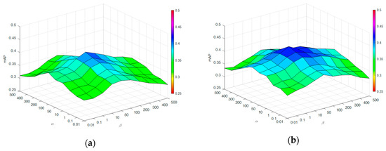
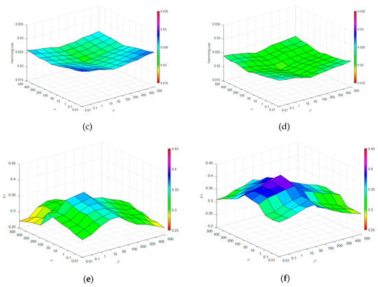
Figure 5.
Impact of regularization parameters α and β: (a) mean average precision on UCMerced dataset; (b) mean average precision on Corel5k dataset; (c) Hamming loss on UCMerced dataset; (d) Hamming loss on Corel5k dataset; (e) F1 score on UCMerced dataset; (f) F1 score on Corel5k dataset.
From these figures, we can observe that when and are both too small, the performances are not satisfactory under the three metrics. With increasing and , the performance improves on both datasets. This proves the importance of the image and label graph. Moreover, optimal results can be achieved when and on the two datasets, although their cardinalities are different. These results demonstrate that the image graph is more important than the label graph in our method, which agrees with Section 5.4.
5.5.2. Impact of Image Similarity Parameter σ
To evaluate the impact of the two image similarities with different weights, we fixed the parameters as , and set the feature dimensions as and . In the implementing procedure, we changed the parameter under different training dataset sizes. Then, we obtained the F1 score results with the top five annotations on the two datasets, which are shown in Figure 6a,b.
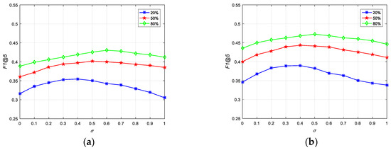
Figure 6.
Impact of : (a) F1 score with different weights of on UCMerced; (b) F1 score with different weights of on Corel5k.
From Figure 6a,b, we can observe that when the training data size is 20% on both datasets, more weight () on image visual similarity can improve the performance significantly, but when it increases to 80%, achieves better values than . According to our analysis, the reason is that, as the training data increases, the semantic information can provide enough useful meaning for the method, which can improve the performance of the algorithm. However, when the image-label matrix is sparse, less information can be obtained from the semantic similarity. It is worth noting that visual similarity can compensate for useful information of this limitation. Another interesting phenomenon is that our method can attain better performance with on the two datasets, when the ratio of training data increases to 50%. Therefore, is a compromise for the two datasets, and can provide a promising result as well.
5.5.3. Impact of Number of Latent Features
There are two other important parameters in our method: The number of latent image features and the number of latent label features . Usually, they are different with good adaptive ability for moderate representations. To study how and affect the performance of our method simultaneously, we conducted a set of experiments on 20% training datasets. varies from 5 to 60 and varies from 5 to 35 on UCMerced, while on Corel5k, the range is from 5 to 60. We fixed the other parameters as and results are shown in Figure 7a,b.
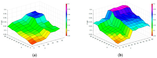
Figure 7.
Impact of the number of feature dimensions: (a) F1@5 with different image feature dimensions and label feature dimensions on UCMerced; (b) F1@5 with different image feature dimensions and label feature dimensions on Corel5k.
It can be seen from Figure 7a,b that the values of F1 score change along with the change of feature dimensionalities. In a certain range, the higher the dimensionality of latent features, the better performance can be achieved. We believe the reason for this is that with more latent features, more information can be represented by the low-rank matrices. However, when and increase to a certain range, the performance is relatively stable. This is because the existing latent features can represent the useful information well. The empirical results show that the ranges are different on the two datasets. On UCMerced, the range is , while on Corel5k it is . There is a fact that large latent features will significantly increase the computation cost. For the overall consideration, we chose relatively smaller values for and to maintain acceptable performance. Thus, we take to get a trade-off for both datasets.
5.5.4. Impact of Regularization Parameter λ
To evaluate the contribution of , we built a set of experiments on both datasets under the F1 score measure, when the training dataset size is 20%, and set the other parameters as . The results are displayed in Figure 8a,b. From these figures, we can see that when the value of is 1 or larger, the F1 score is better. This means larger can achieve better F1 scores. Additionally, when , the proposed method can get the best performance on both datasets. However, too-large can result in much computation cost. Considering this, we take in our experiments as a trade-off.
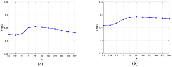
Figure 8.
Impact of parameter : (a) F1 score with different on UCMerced; (b) F1 score with different on Corel5k.
6. Discussion
To assess the efficiency of the proposed method, several qualitative comparison experiments were done on the UCMerced and Corel5k datasets. We utilized five metrics to evaluate the performance of all approaches. Meanwhile, to evaluate the robustness of the proposed method, we deployed these experiments on training datasets of different sizes. The results and analyses are described in Section 5.3.1, Section 5.3.2, and Section 5.3.3.
It can be seen from these results that our method outperforms the baseline methods under most metrics on both datasets, especially when the dataset is sparse. Precision is boosted significantly on the UCMerced dataset, which confirms the advantage of using the image graph and label graph simultaneously. Moreover, recall is improved by a large margin on the Corel5K dataset. This is because this dataset has fewer labels per image and more accurate labels can be covered by the proposed method. Furthermore, recall and precision affect the value of F1 score simultaneously, which is more sensitive for performance. Nevertheless, our method still achieves the best F1 score on both datasets, even more on the different sizes of training data. According to our analysis, when the ratio of training data increases, more information can be obtained from the dataset; e.g., more label information can be obtained from UCMerced dataset. Also, we can obtain more image information from both datasets, therefore F1 improves. Hamming loss and mean average precision metrics quantify the overall performance of the methods. Our method achieves better performance under these two metrics on both datasets, which proves the effectiveness of the proposed method.
In the compared methods, MLC-LRR achieves relatively better performance on both datasets; specifically, when the ratio of labeled images on UCMerced increases to 50% and 80%, it achieves better values in recall than our method. Also, it attains better precision and Hamming loss values on Corel5k than our method when the ratio of labeled images increases to 80%. This proves that there is an advantage to using the feature graph and semantic graph simultaneously. However, the limitations of this method are that it depends heavily on the ratio of labeled images and does not consider the semantic gap between low-level features and high-level features. On the other hand, this method has a rather more complicated process than our method. Our method overcomes these limitations by introducing both the visual content and semantic similarities to reduce the semantic gap and have a simpler framework. Among these methods, MLLS performs worst on the two datasets due to the limitation of only using label correlation in image annotation. By using a bi-relational semantic graph for images and labels, BG performs better, ignoring the visual content of the images. MRF and MMP achieve rather good results on both datasets by making full use of the image features. MMP achieves many improvements on Corel5k because of the multi-view features of images. Extracting more features can improve the overall performance of the method. However, more features can result in more dimensionality problems. It increases the computation cost and storage burden. ECC uses more classifiers to improve the performance, which increases the computation cost. Computation efficiency is also a challenging issue for the RAkEL approach, although it achieves rather good performance on both datasets. MLNRS gets a better result than the others except MLC-LRR, which provides the advantage of considering the semantic neighborhood rough sets, but it does not consider the visual content of images, and the process of finding the nearest neighbors will be too time-consuming.
Although our method achieved the best performance in the experiments, there are several limitations. First, to solve the sparsity problem of the input matrix, we introduced the weighted matrix, which increased the computation cost of this method. The running time proved that it is not a very quick method. Second, to find the best performance for different datasets, we need to tune the parameters very carefully, which is also time-consuming.
Nevertheless, these experimental results indicate that our method outperformed most of the methods under most of the metrics. It has the advantages of simplicity, high efficiency, low storage cost, scalability, and strong robustness. It is suitable for not only remote sensing multi-label annotation tasks but also the natural multi-label image annotation problem.
7. Conclusions and Future Works
In this paper, we proposed the WDG-NMTF, a novel method to solve the remote sensing multi-label annotation problem. This method seamlessly combines matrix factorization and image annotation, utilizing both the high efficiency and scalability of matrix factorization for image annotation. To improve the performance of the method, we employed both image and label graphs to extend the NMTF. Moreover, to reduce the semantic gap between images and labels, we used both low-level and high-level features of images to make full use of the hidden semantics and image content information in datasets. Generally speaking, using this method will make remote sensing image labeling more efficient and less labor-intensive, especially for huge numbers of unlabeled images. Experimental results on benchmark datasets demonstrated that the proposed method performs better than most state-of-the-art multi-label annotation methods.
In the future, we will investigate how to accelerate the method during the updating process. Moreover, we will reduce the computation cost resulting from the introduction of weighted matrix, which is calculated at each step of iteration. It is worth developing a more efficient multi-label annotation method in terms of both accuracy and computation in the future.
Author Contributions
All authors extensively discussed the contents of this paper and contributed to its preparation. J.Z. (Juli Zhang) conceived and designed the experiments, and wrote the paper; J.Z. (Junyi Zhang) implemented the experiments; T.D. analyzed the data and reviewed the paper; Z.H. supervised the study and reviewed the manuscript.
Funding
This research was funded by China Youth Science Foundation, grant number 61702413, and the Technology Innovation Funds for the Ninth Academy of China Aerospace, grant number 2016JY06.
Acknowledgments
The authors thank everyone who contributed to this work. We gratefully thank Xuehan Tang, Zhuping Wang, Lan Liu and Zhong Ma for their sincere support in our work. We also thank all the anonymous reviewers and editors for their helpful comments and suggestions.
Conflicts of Interest
The authors declare that there are no conflict of interest regarding the publication of this paper.
Appendix A
To prove Theorem 1, we need to show that the object function in Equation (4) is nonincreasing under the steps in Equations (7)–(9) and converges to a local minimum, respectively. We follow a scheme similar to that described in [57]. We begin with the definition of auxiliary function.
Definition 1.
is an auxiliary function for if the following conditions are satisfied:
The auxiliary function is very useful thanks to the following lemma:
Lemma 1
[57].If is the auxiliary function of , then is nonincreasing under the following update rule:
where is the update iteration of H.
Because , is monotonically decreasing. Therefore, the key is to find a proper auxiliary function for . To construct the auxiliary functions for these objective functions, we employ the following propositions:
Lemma 2
[65].For any matrices , we have the following inequality:
Lemma 3
[21].For any non-negative matrices , where M and N are symmetric matrices, we have the following inequality:
Lemma 4
[65].For any symmetric matrix , and any matrices , we have the following inequality:
Lemma 5
(quadratic lower bound) [65].For , we have the following inequality:
Due to the alternatively updating rules, we prove that each rule leads the objective function to converge to a local minimum. We first proved the object function in Equation (4) with respect to being non-increasing under the steps in Equation (7) and converging to a local minimum.
First, we write the objective function in Equation (4) with respect to as
Second, we prove that the following function is an auxiliary function of :
Since is obvious when , we only need to show that . We can find that: (a) the first term in is always smaller than the first term in , due to Lemma 2; (b) the second term in is always bigger than the second term in , due to Lemma 3; (c) the third term in is always bigger than the third term in , due to Lemma 4; and (d) the fourth term in is always smaller than the fourth term in , due to Lemma 5. By summing over all the bounds, we get . Thus, the conditions of Definition 1 are satisfied. is an auxiliary function of .
Third, we prove is a convex function in and it has a local minimum.
To prove it is convex, we calculate the first derivative of
Then we have the Hessian matrix as
It can be seen that the above matrix is a diagonal matrix with positive diagonal elements, where are the functions that equal 1 when or and 0 otherwise. Moreover, . Therefore, is a convex function. We can find a local minimum of by fixing and setting the first derivative of equal to zero. After solving it for , we get the minimum as
According to Lemma 1, and , and we recover Equation (7). Under this update rule, decreases monotonically and converges to a local minimum.
With respect to updating rules in Equations (8) and (9), the proofs are analogous to Equation (7).
In summary, we have proved the convergence of Theorem 1.
References
- Xu, G.; Shen, W.; Wang, X. Applications of wireless sensor networks in marine environment monitoring: a survey. Sensors 2014, 14, 16932–16954. [Google Scholar] [CrossRef]
- Chaudhuri, B.; Demir, B.; Chaudhuri, S.; Bruzzone, L. Multilabel Remote Sensing Image Retrieval Using a Semisupervised Graph-Theoretic Method. IEEE Trans. Geosci. Remote Sens. 2017, 1114–1158. [Google Scholar] [CrossRef]
- Karalas, K.; Tsagkatakis, G.; Zervakis, M.; Tsakalides, P. Land Classification Using Remotely Sensed Data: Going Multilabel. IEEE Trans. Geosci. Remote Sens. 2016, 54, 3548–3563. [Google Scholar] [CrossRef]
- Li, D. Content-based remote sensing image retrieval. Proc. SPIE Int. Soc. Opt. Eng. 2005, 6044, 60440Q. [Google Scholar] [CrossRef]
- Demir, B.; Bruzzo, L. Kernel-based hashing for content-based image retrval in large remote sensing data archive. In Proceedings of the 2014 IEEE International Geoscience and Remote Sensing Symposium (IGARSS), Quebec City, QC, Canada, 13–18 July 2014; pp. 3542–3545. [Google Scholar]
- Demir, B.; Bruzzone, L. A Novel Active Learning Method in Relevance Feedback for Content-Based Remote Sensing Image Retrieval. IEEE Trans. Geosci. Remote Sens. 2015, 53, 2323–2334. [Google Scholar] [CrossRef]
- Smeulders, A.W.M.; Worring, M.; Santini, S.; Gupta, A.; Jain, R.C. Content-based image retrieval at the end of the early years. IEEE Trans. Pattern Anal. Mach. Intell. 2000, 22, 1349–1380. [Google Scholar] [CrossRef]
- Hao, M.; Zhu, J.; Lyu, R.T.; King, I. Bridging the Semantic Gap Between Image Contents and Tags. IEEE Trans. Multimed. 2010, 12, 462–473. [Google Scholar] [CrossRef]
- Luo, W.; Li, H.; Liu, G. Automatic Annotation of Multispectral Satellite Images Using Author–Topic Model. IEEE Geosci. Remote Sens. Lett. 2012, 9, 634–638. [Google Scholar] [CrossRef]
- Yao, X.; Han, J.; Cheng, G.; Qian, X.; Guo, L. Semantic Annotation of High-Resolution Satellite Images via Weakly Supervised Learning. IEEE Trans. Geosci. Remote Sens. 2016, 54, 3660–3671. [Google Scholar] [CrossRef]
- Chen, K.; Jian, P.; Zhou, Z.; Guo, J.; Zhang, D. Semantic Annotation of High-Resolution Remote Sensing Images via Gaussian Process Multi-Instance Multilabel Learning. IEEE Geosci. Remote Sens. Lett. 2013, 10, 1285–1289. [Google Scholar] [CrossRef]
- Luo, W.; Li, H.; Liu, G.; Zeng, L. Semantic Annotation of Satellite Images Using Author–Genre–Topic Model. IEEE Trans. Geosci. Remote Sens. 2013, 52, 1356–1368. [Google Scholar] [CrossRef]
- Lee, D.D.; Seung, H.S. Learning the parts of objects by non-negative matrix factorization. Nature 1999, 401, 788–791. [Google Scholar] [CrossRef]
- Gu, Q.; Zhou, J.; Ding, C.H.Q. Collaborative Filtering: Weighted Nonnegative Matrix Factorization Incorporating User and Item Graphs. In Proceedings of the 10th SIAM International Conference on Data Mining, SDM 2010, Columbus, OH, USA, 29 April–1 May 2010; pp. 199–210. [Google Scholar]
- Hernando, A.; Ortega, F. A non-negative matrix factorization for collaborative filtering recommender systems based on a Bayesian probabilistic model. Knowl.-Based Syst. 2016, 97, 188–202. [Google Scholar] [CrossRef]
- Li, Y.; Wang, D.; He, H.; Jiao, L.; Xue, Y. Mining intrinsic information by matrix factorization-based approaches for collaborative filtering in recommender systems. Neurocomputing 2017, 249, 48–63. [Google Scholar] [CrossRef]
- Kalayeh, M.M.; Idrees, H.; Shah, M. NMF-KNN: Image Annotation Using Weighted Multi-view Non-negative Matrix Factorization. In Proceedings of the IEEE Conference on Computer Vision and Pattern Recognition, Columbus, OH, USA, 24–27 June 2014; pp. 184–191. [Google Scholar]
- Jia, X.; Sun, F.; Li, H.; Cao, Y.; Zhang, X. Image Multi-Label Annotation Based on Supervised Nonnegative Matrix Factorization with New Matching Measurement. Neurocomputing 2017, 219, 518–525. [Google Scholar] [CrossRef]
- Rad, R.; Jamzad, M. Image Annotation using Multi-view Non-negative Matrix Factorization with Different Number of Basis Vectors. J. Vis. Commun. Image Represent. 2017, 46, 1–12. [Google Scholar] [CrossRef]
- Ge, H.; Yan, Z.; Dou, J.; Wang, Z.; Wang, Z. A Semisupervised Framework for Automatic Image Annotation Based on Graph Embedding and Multiview Nonnegative Matrix Factorization. Math. Probl. Eng. 2018, 2018, 1–11. [Google Scholar] [CrossRef]
- Ding, C.H.Q.; Li, T.; Peng, W.; Park, H. Orthogonal nonnegative matrix t-factorizations for clustering. In Proceedings of the Twelfth ACM SIGKDD International Conference on Knowledge Discovery and Data Ming, Philadelphia, PA, USA, 20–23 August 2006; pp. 126–135. [Google Scholar]
- Yoo, J.; Choi, S. Weighted Nonnegative Matrix Co-Tri-Factorization for Collaborative Prediction. In Proceedings of the 1st Asian Conference on Machine Learning: Advances in Machine Learning, Nanjing, China, 2–4 November 2009; pp. 396–411. [Google Scholar]
- Chen, G.; Wang, F.; Zhang, C. Collaborative filtering using orthogonal nonnegative matrix tri-factorization. Inf. Process. Manag. 2009, 45, 368–379. [Google Scholar] [CrossRef]
- Lienou, M.; Maitre, H.; Datcu, M. Semantic Annotation of Satellite Images Using Latent Dirichlet Allocation. IEEE Geosci. Remote Sens. Lett. 2010, 7, 28–32. [Google Scholar] [CrossRef]
- Zhou, N.; Cheung, W.K.; Qiu, G.; Xue, X. A Hybrid Probabilistic Model for Unified Collaborative and Content-Based Image Tagging. IEEE Trans. Pattern Anal. Mach. Intell. 2011, 33, 1281–1294. [Google Scholar] [CrossRef]
- Liu, H.; Wu, Z.; Cai, D.; Huang, T.S. Constrained Nonnegative Matrix Factorization for Image Representation. IEEE Trans. Pattern Anal. Mach. Intell. 2012, 34, 1299–1311. [Google Scholar] [CrossRef]
- Wu, L.; Jin, R.; Jain, A.K. Tag Completion for Image Retrieval. IEEE Trans. Pattern Anal. Mach. Intell. 2013, 35, 716–727. [Google Scholar] [CrossRef]
- Carneiro, G.; Chan, A.B.; Moreno, P.J.; Vasconcelos, N. Supervised Learning of Semantic Classes for Image Annotation and Retrieval. IEEE Trans. Pattern Anal. Mach. Intell. 2007, 29, 394–410. [Google Scholar] [CrossRef]
- Tieu, K.; Viola, P. Boosting image retrieval. In Proceedings of the Computer Vision and Pattern Recognition, Hilton Head, SC, USA, 13–15 June 2000; pp. 228–235. [Google Scholar]
- Yu, Y.; Pedrycz, W.; Miao, D. Neighborhood rough sets based multi-label classification for automatic image annotation. Int. J. Approx. Reason. 2013, 54, 1373–1387. [Google Scholar] [CrossRef]
- Fei, W.; Han, Y.; Qi, T.; Zhuang, Y. Multi-label boosting for image annotation by structural grouping sparsity. In Proceedings of the 18th ACM International Conference on Multimedea, Firenze, Italy, 25–29 October 2010; pp. 15–24. [Google Scholar] [CrossRef]
- Briggs, F.; Fern, X.Z.; Raich, R.; Lou, Q. Instance Annotation for Multi-Instance Multi-Label Learning. ACM Trans. Knowl. Discov. Data 2013, 7, 1–30. [Google Scholar] [CrossRef]
- Zhang, H.; Berg, A.C.; Maire, M.; Malik, J. SVM-KNN: Discriminative Nearest Neighbor Classification for Visual Category Recognition. In Proceedings of the 2006 IEEE Computer Society Conference on Computer Vision and Pattern Recognition, New York, NY, USA, 17–22 June 2006; Volume 2, pp. 2126–2136. [Google Scholar] [CrossRef]
- Tan, Q.; Liu, Y.; Chen, X.; Yu, G. Multi-Label Classification Based on Low Rank Representation for Image Annotation. Remote Sens. 2017, 9, 109. [Google Scholar] [CrossRef]
- Karalas, K.; Tsagkatakis, G. Deep learning for multi-label land cover classification. In Proceedings of the SPIE Remote Sensing XXI, Toulouse, France, 21–24 September 2015; Volume 9643, p. 96430Q. [Google Scholar]
- Sharifi, Z.; Rezghi, M.; Nasiri, M. A new algorithm for solving data sparsity problem based-on Non negative matrix factorization in recommender systems. In Proceedings of the 4th International Econference on Computer and Knowledge Engineering, Mashhad, Iran, 29–30 October 2014; pp. 56–61. [Google Scholar] [CrossRef]
- Tommi, N.; Jaakkola, S. Maximum-Margin Matrix Factorization. Adv. Nips 2005, 37, 1329–1336. [Google Scholar]
- Talwalkar, A.; Kumar, S.; Mohri, M.; Rowley, H. Large-scale SVD and manifold learning. J. Mach. Learn. Res. 2013, 14, 3129–3152. [Google Scholar] [CrossRef]
- Kim, Y.D.; Choi, S. Weighted nonnegative matrix factorization. In Proceedings of the IEEE International Conference on Acoustics, Speech and Signal Processing, Taipei, Taiwan, 19–24 April 2009; pp. 1541–1544. [Google Scholar] [CrossRef]
- Cai, D.; He, X.; Han, J.; Huang, T.S. Graph Regularized Nonnegative Matrix Factorization for Data Representation. IEEE Trans. Pattern Anal. Mach. Intell. 2011, 33, 1548–1560. [Google Scholar] [CrossRef]
- Li, H.; Zhang, J.; Liu, J. Graph-regularized CF with local coordinate for image representation. J. Vis. Commun. Image Represent. 2017, 49, 392–400. [Google Scholar] [CrossRef]
- Shang, F.; Jiao, L.C.; Wang, F. Graph dual regularization non-negative matrix factorization for co-clustering. Pattern Recognit. 2012, 45, 2237–2250. [Google Scholar] [CrossRef]
- Ye, J.; Jin, Z. Dual-graph regularized concept factorization for clustering. Neurocomputing 2014, 138, 120–130. [Google Scholar] [CrossRef]
- Yin, M.; Gao, J.; Lin, Z.; Shi, Q.; Guo, Y. Dual Graph Regularized Latent Low-Rank Representation for Subspace Clustering. IEEE Trans. Image Process. 2015, 24, 4918–4933. [Google Scholar] [CrossRef]
- Li, X.; Cui, G.; Dong, Y. Graph Regularized Non-Negative Low-Rank Matrix Factorization for Image Clustering. IEEE Trans. Syst. Man Cybern. 2017, 47, 3840–3853. [Google Scholar] [CrossRef]
- Hua, W.; Nie, F.; Huang, H.; Makedon, F. Fast Nonnegative Matrix Tri-Factorization for Large-Scale Data Co-Clustering. In Proceedings of the 22nd International Joint Conference on Artificial Intelligence, Barcelona, Spain, 19–22 July 2011. [Google Scholar]
- Buono, N.D.; Pio, G. Non-negative Matrix Tri-Factorization for co-clustering: An analysis of the block matrix. Inf. Sci. 2015, 301, 13–26. [Google Scholar] [CrossRef]
- Ma, H.; Zhao, W.; Tan, Q.; Shi, Z. Orthogonal Nonnegative Matrix Tri-factorization for Semi-supervised Document Co-clustering. Adv. Knowl. Discov. Data Min. 2010, 6119, 189–200. [Google Scholar] [CrossRef]
- Pei, Y.; Chakraborty, N.; Sycara, K. Nonnegative matrix tri-factorization with graph regularization for community detection in social networks. In Proceedings of the 24th International Conference on Artificial Intelligence, Buenos Aires, Argentina, 25–31 July 2015. [Google Scholar]
- Merris, R. Laplacian matrices of graphs: A survey. Linear Algebra Its Appl. 1994, 197–198, 143–176. [Google Scholar] [CrossRef]
- Guillaumin, M.; Mensink, T.; Verbeek, J.; Schmid, C. TagProp: Discriminative Metric Learning in Nearest Neighbor Models for Image Auto-Annotation. In Proceedings of the 12th IEEE International Conference on Computer Vision, Kyoto, Japan, 29 September–2 October 2010. [Google Scholar]
- Oliva, A.; Torralba, A. Modeling the Shape of the Scene: A Holistic Representation of the Spatial Envelope. Int. J. Comput. Vis. 2001, 42, 145–175. [Google Scholar] [CrossRef]
- Lowe, D.G. Distinctive Image Features from Scale-Invariant Keypoints. Int. J. Comput. Vis. 2004, 60, 91–110. [Google Scholar] [CrossRef]
- Weijer, J.V.D.; Schmid, C. Coloring Local Feature Extraction. In Proceedings of the 9th European Conference on Computer Vision, Graz, Austria, 7–13 May 2006. [Google Scholar]
- Hua, W.; Huang, H.; Ding, C. Multi-label Feature Transform for Image Classifications. In Proceedings of the 11th European Conference on Computer Vision, Heraklion, Greece, 5–11 September 2010. [Google Scholar]
- Boyd, S.; Vandenberghe, L. Convex Optimization. IEEE Trans. Autom. Control 2006, 51, 1859. [Google Scholar] [CrossRef]
- Lee, D.D.; Seung, H.S. Algorithms for Non-Negative Matrix Factorization; NIPS; MIT Press: Cambridge, MA, USA, 2000; pp. 556–562. [Google Scholar]
- Grangier, D.; Bengio, S. A Discriminative Kernel-Based Approach to Rank Images from Text Queries. IEEE Trans. Pattern Anal. Mach. Intell. 2008, 30, 1371–1384. [Google Scholar] [CrossRef]
- Ji, S.; Tang, L.; Yu, S.; Ye, J. A shared-subspace learning framework for multi-label classification. Acm Trans. Knowl. Discov. Data 2010, 4, 1–29. [Google Scholar] [CrossRef]
- Wang, H.; Huang, H.; Ding, C. Image annotation using bi-relational graph of images and semantic labels. In Proceedings of the Computer Vision and Pattern Recognition, Colorado Springs, CO, USA, 20–25 June 2011. [Google Scholar]
- Kong, D.; Ding, C.; Huang, H.; Zhao, H. Multi-label ReliefF and F-statistic feature selections for image annotation. In Proceedings of the IEEE Conference on Computer Vision and Pattern Recognition, Providence, RI, USA, 16–21 June 2012. [Google Scholar]
- He, Z.; Chen, C.; Bu, J.; Li, P.; Cai, D. Multi-view based multi-label propagation for image annotation. Neurocomputing 2015, 168, 853–860. [Google Scholar] [CrossRef]
- Read, J.; Pfahringer, B.; Holmes, G.; Frank, E. Classifier chains for multi-label classification. Mach. Learn. 2011, 85, 333. [Google Scholar] [CrossRef]
- Tsoumakas, G.; Katakis, I.; Vlahavas, I. Random k-Labelsets for Multilabel Classification. IEEE Trans. Knowl. Data Eng. 2011, 23, 1079–1089. [Google Scholar] [CrossRef]
- Yang, Z.; Oja, E. Linear and nonlinear projective nonnegative matrix factorization. IEEE Trans Neural Netw 2010, 21, 734–749. [Google Scholar] [CrossRef] [PubMed]
© 2019 by the authors. Licensee MDPI, Basel, Switzerland. This article is an open access article distributed under the terms and conditions of the Creative Commons Attribution (CC BY) license (http://creativecommons.org/licenses/by/4.0/).