Assessment of Individual Tree Detection and Canopy Cover Estimation using Unmanned Aerial Vehicle based Light Detection and Ranging (UAV-LiDAR) Data in Planted Forests


Abstract

1. Introduction
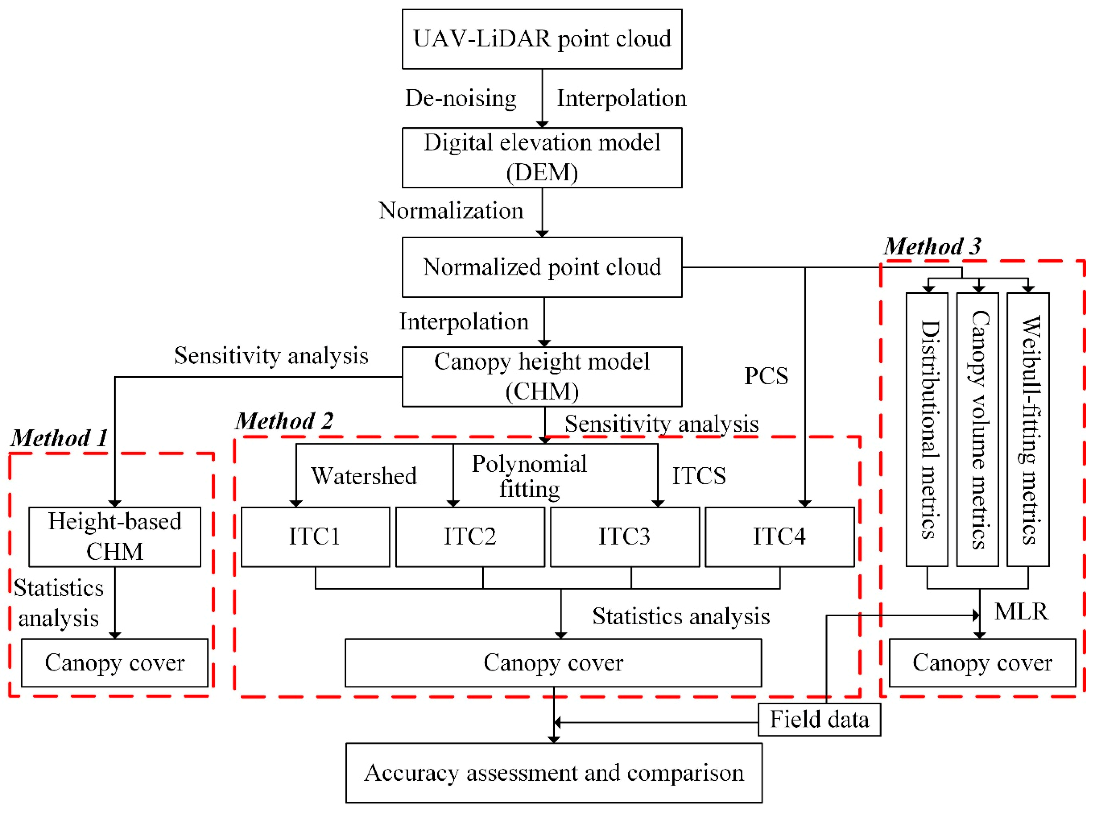
2. Materials and Methods
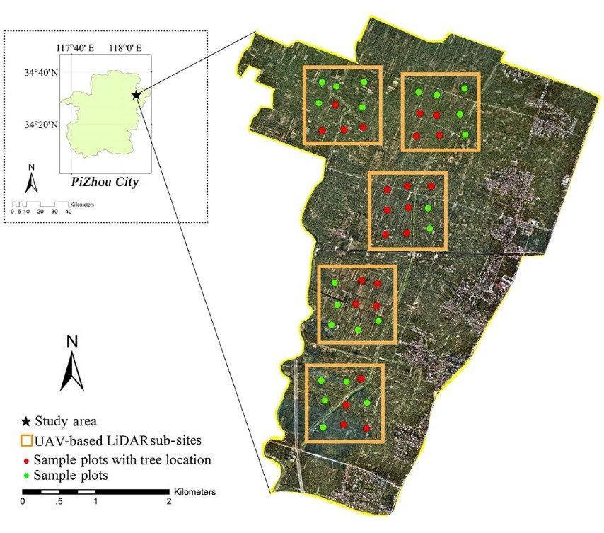
2.1. Study Area
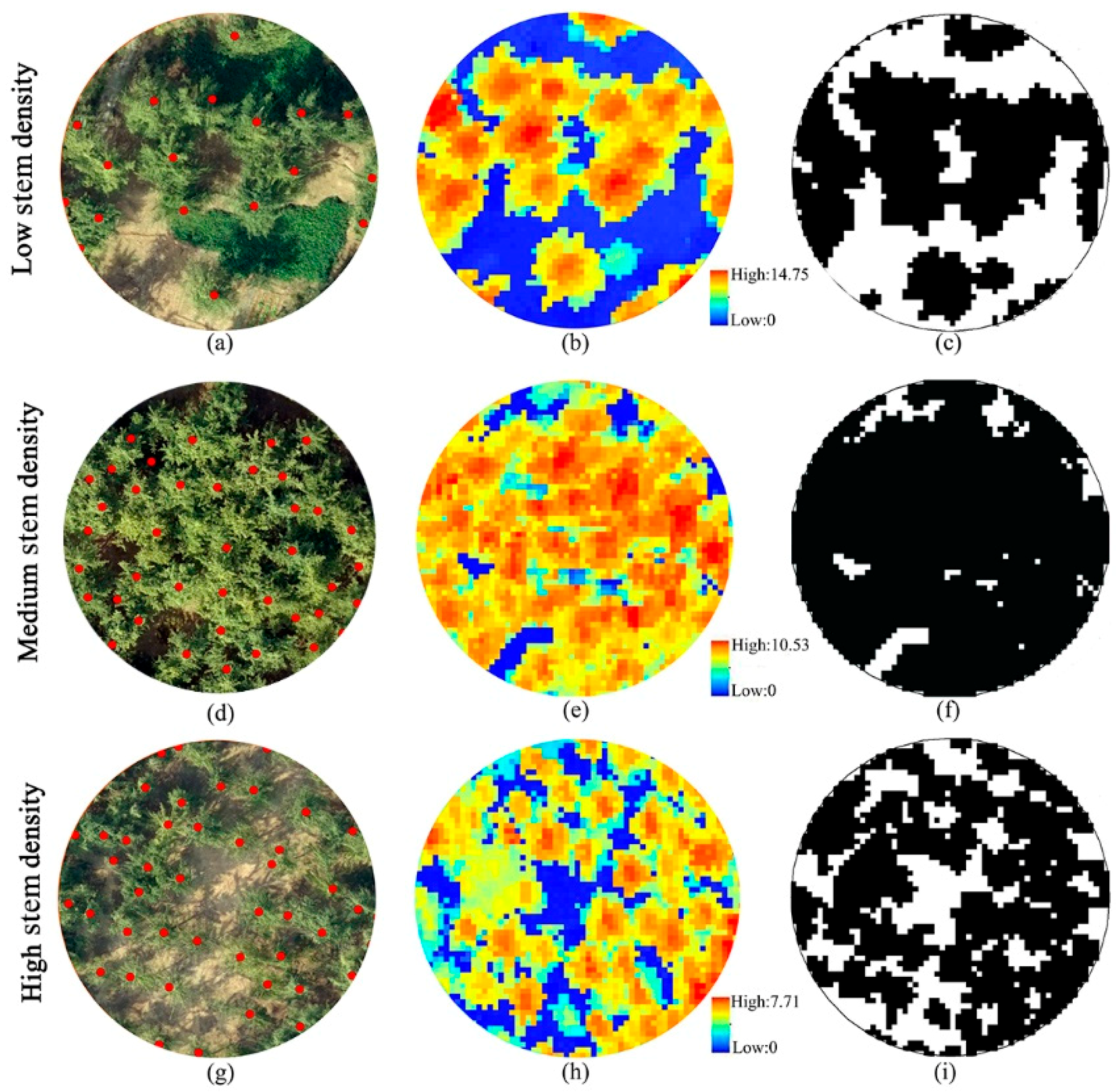
2.2. Field Data
2.3. LiDAR Data Acquisition and Preprocessing
2.4. LiDAR Metrics Calculation
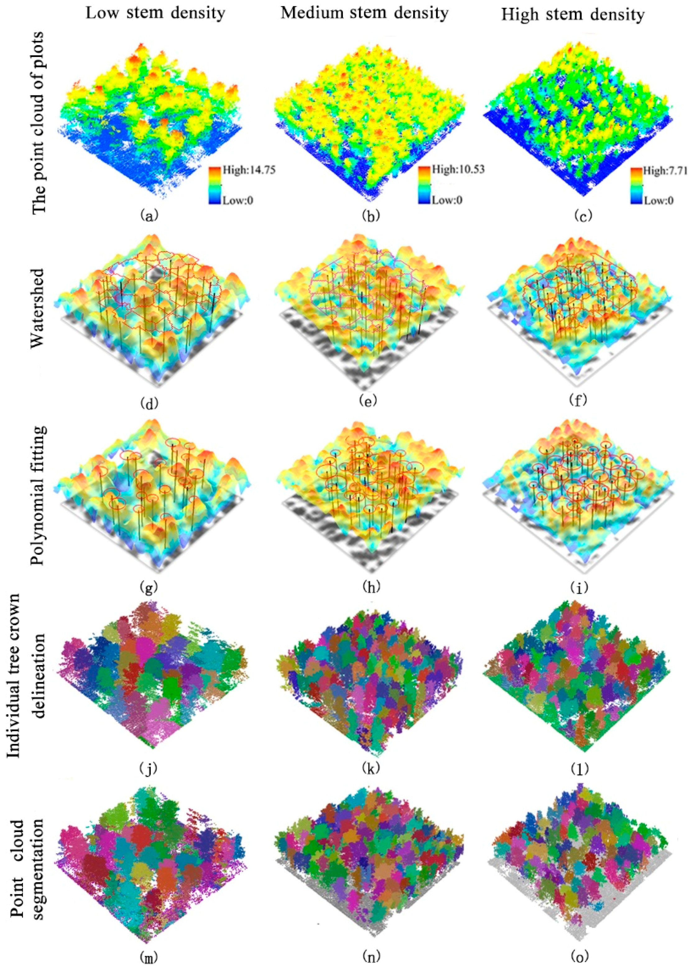
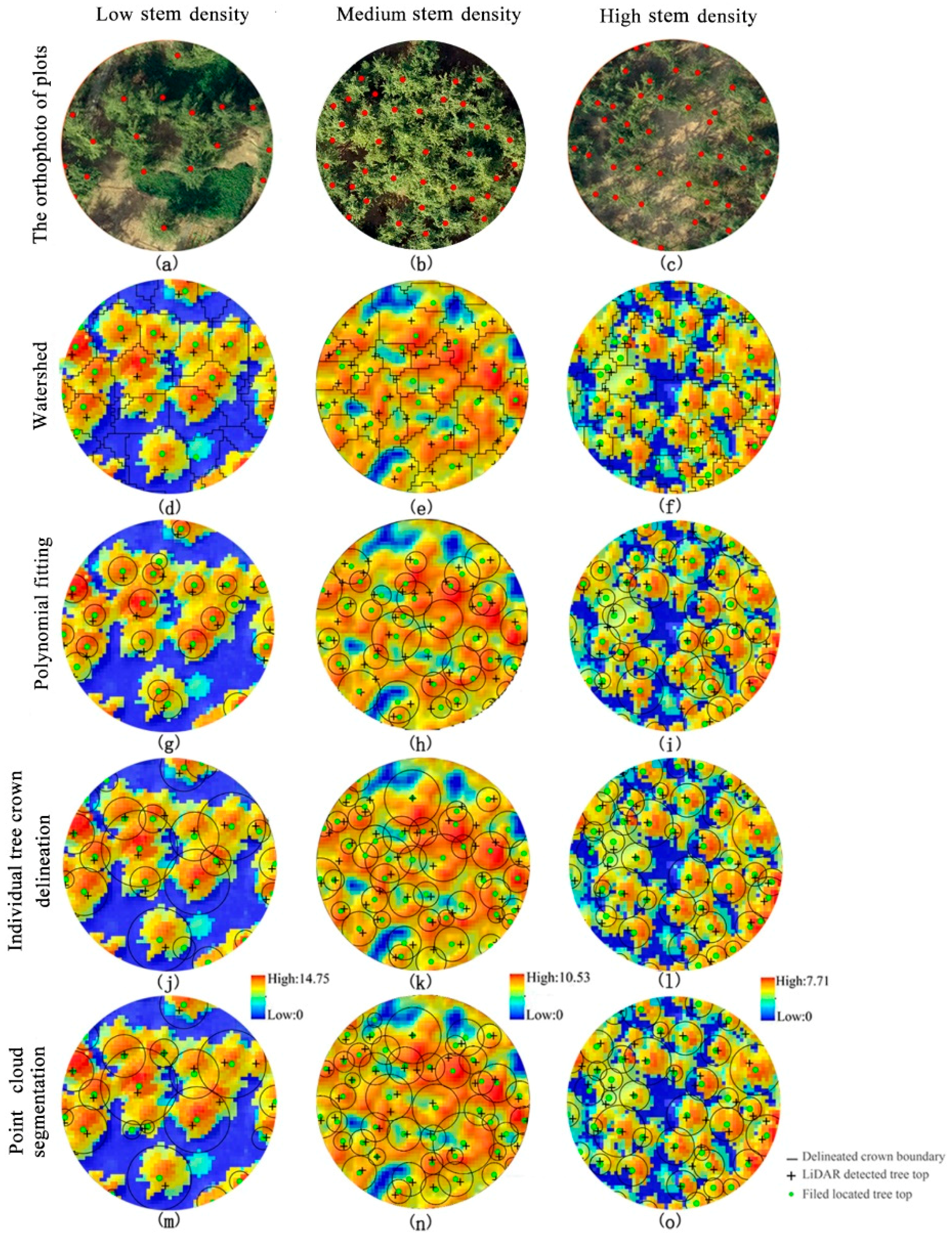
2.5. Individual Tree Segmentation Method
2.5.1. Watershed Algorithm
2.5.2. Polynomial Fitting Method
2.5.3. Individual Tree Crown Segmentation (ITCS)
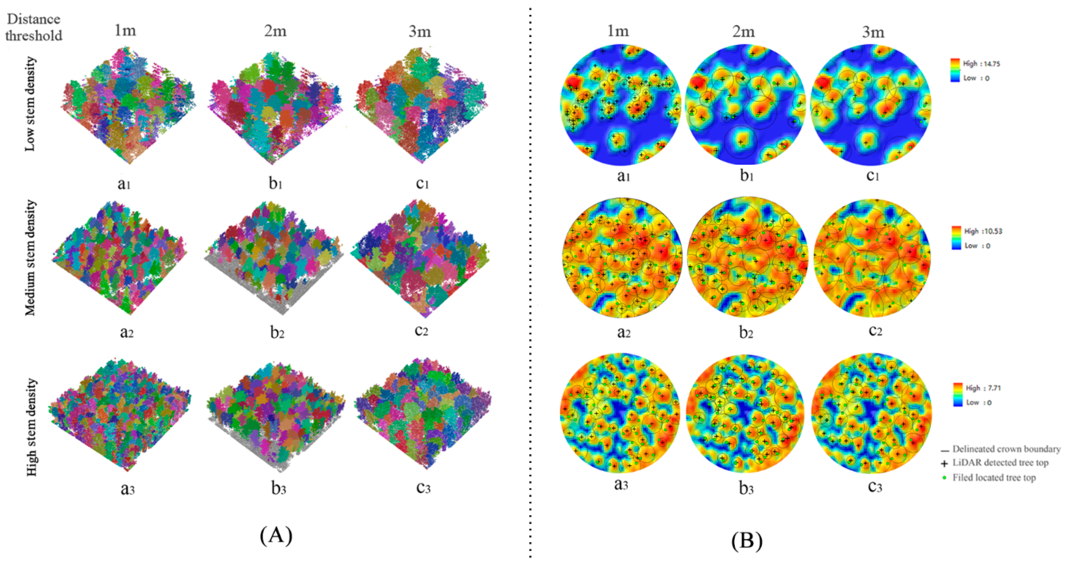
2.5.4. Point Cloud Segmentation (PCS)
2.6. Indicators of Individual Tree Segmentation Accuracy
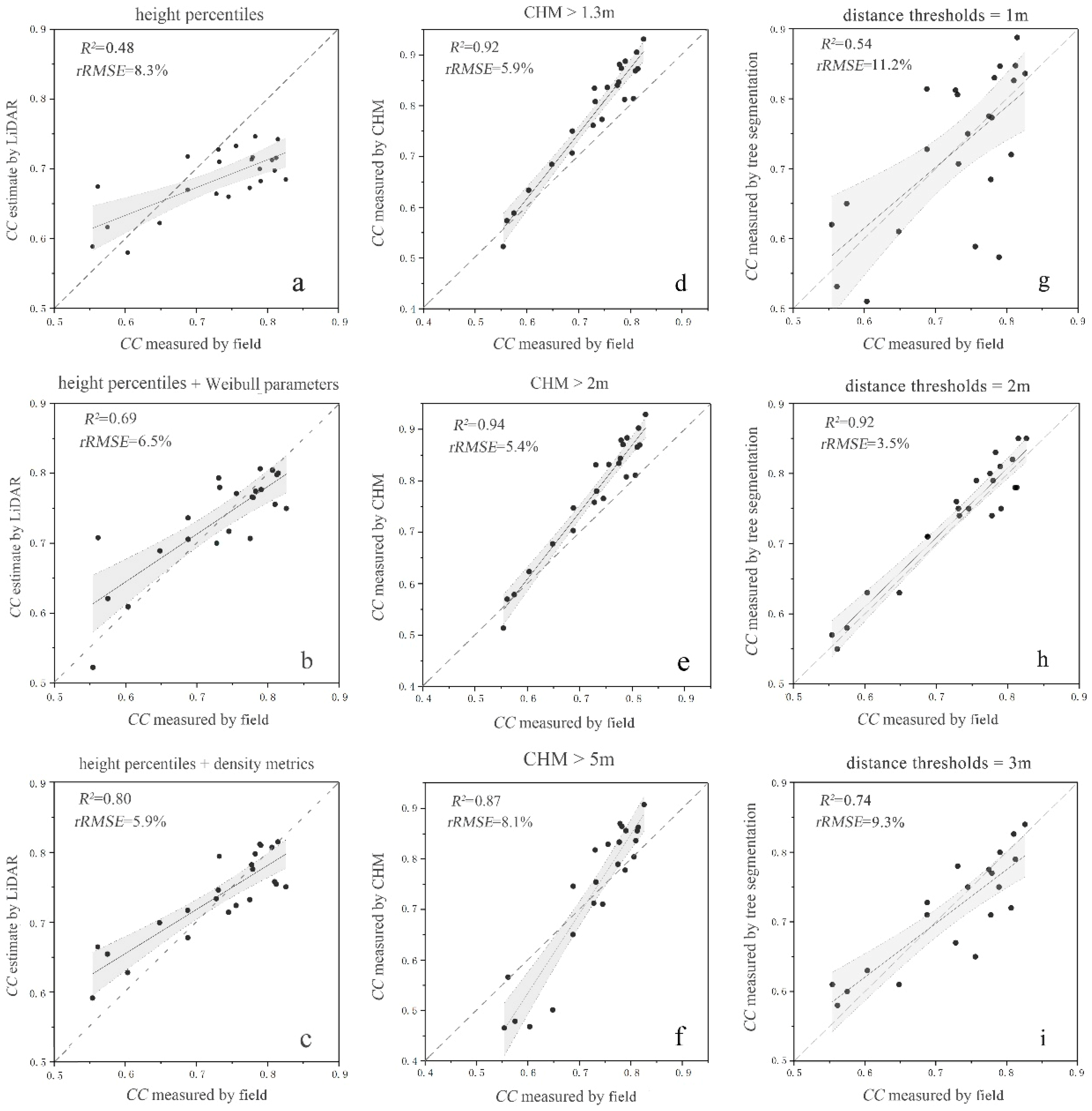
2.7. Estimation of Forest Canopy Cover by the Individual Tree Segmentation-Based Method
2.8. Estimation of Forest Canopy Cover by the CHM-based Method
2.9. Estimation of Forest Canopy Cover by the LiDAR Metrics Statistics Model
2.10. Model Accuracy Evaluation
3. Results
4. Discussion
5. Conclusions
Author Contributions
Funding
Acknowledgments
Conflicts of Interest
References
- Brockerhoff, E.G.; Jactel, H.; Parrotta, J.A.; Quine, C.P.; Sayer, J. Plantation forests and biodiversity: Oxymoron or opportunity? Biodivers. Conserv. 2008, 17, 925–951. [Google Scholar] [CrossRef]
- Society, B.E.; Harper, J.L. A Darwinian Approach to Plant Ecology. J. Appl. Ecol. 1967, 4, 267–290. [Google Scholar]
- Hartley, M.J. Rationale and methods for conserving biodiversity in plantation forests. Ecol. Manag. 2002, 155, 81–95. [Google Scholar] [CrossRef]
- Food and Agriculture Organization of the United Nations (FAO). Global Forest Resources Assessment 2010; FAO: Rome, Italy, 2010. [Google Scholar]
- Sun, Y.; Liang, X.; Liang, Z.; Welham, C.; Li, W. Deriving Merchantable Volume in Poplar through a Localized Tapering Function from Non-Destructive Terrestrial Laser Scanning. Forests 2016, 7, 87. [Google Scholar] [CrossRef]
- Gong, W.; Chen, C.; Dobeš, C.; Fu, C.X.; Koch, M.A. Phylogeography of a living fossil: Pleistocene glaciations forced Ginkgo biloba L. (Ginkgoaceae) into two refuge areas in China with limited subsequent postglacial expansion. Mol. Phylogenet. Evol. 2008, 48, 1094–1105. [Google Scholar] [CrossRef] [PubMed]
- Fuliang, C. Chinese Ginkgo; China Forestry Publishing House: Beijing, China, 2007. [Google Scholar]
- Xu, M.; Qi, Y. Soil surface CO2 efflux and its spatial and temporal variations in a young ponderosa pine plantation in northern California. Glob. Chang. Biol. 2001, 7, 667–677. [Google Scholar] [CrossRef]
- Barlow, J.; Gardner, T.A.; Araujo, I.S.; Avila-Pires, T.C.; Bonaldo, A.B.; Costa, J.E.; Esposito, M.C.; Ferreira, L.V.; Hawes, J.; Hernandez, M.I.M.; et al. Quantifying the biodiversity value of tropical primary, secondary, and plantation forests. Proc. Natl. Acad. Sci. USA 2007, 104, 18555–18560. [Google Scholar] [CrossRef]
- Moeser, D.; Roubinek, J.; Schleppi, P.; Morsdorf, F.; Jonas, T. Canopy closure, LAI and radiation transfer from airborne LiDAR synthetic images. Agric. Meteorol. 2014, 197, 158–168. [Google Scholar] [CrossRef]
- Zhu, G.; Ju, W.; Chen, J.M.; Gong, P.; Xing, B.; Zhu, J. Foliage clumping index over China’s landmass retrieved from the MODIS BRDF parameters product. IEEE Trans. Geosci. Remote Sens. 2012, 50, 2122–2137. [Google Scholar] [CrossRef]
- Food and Agriculture Organization of the United Nations (FAO). Forest Resource Assessment; FAO: Rome, Italy, 2005. [Google Scholar]
- Jennings, S. Assessing forest canopies and understorey illumination: Canopy closure, canopy cover and other measures. Forestry 1999, 72, 59–74. [Google Scholar] [CrossRef]
- Hansen, M.C.; Potapov, P.V.; Moore, R.; Hancher, M.; Turubanova, S.A.; Tyukavina, A.; Thau, D.; Stehman, S.V.V.; Goetz, S.J.J.; Loveland, T.R.R.; et al. High-Resolution Global Maps of 21st-Century Forest Cover Change. Science 2013, 342, 850–854. [Google Scholar] [CrossRef] [PubMed]
- Li, M.S.; Mao, L.J.; Shen, W.J.; Liu, S.Q.; Wei, A.S. Change and fragmentation trends of Zhanjiang mangrove forests in southern China using multi-temporal Landsat imagery (1977 e 2010). Estuar. Coast. Shelf Sci. 2013, 130, 111–120. [Google Scholar] [CrossRef]
- Chianucci, F.; Disperati, L.; Guzzi, D.; Bianchini, D.; Nardino, V.; Lastri, C.; Rindinella, A.; Corona, P. Estimation of canopy attributes in beech forests using true colour digital images from a small fixed-wing UAV. Int. J. Appl. Earth Obs. Geoinf. 2016, 47, 60–68. [Google Scholar] [CrossRef]
- Cook, J.G.; Stutzman, T.W.; Bowers, C.W.; Brenner, K.A.; Irwin, L.L. Spherical densiometers produce biased estimates of forest canopy cover. Wildl. Soc. Bull. 1995, 23, 711–717. [Google Scholar] [CrossRef]
- Korhonen, L.; Korhonen, K.T.; Rautiainen, M.; Stenberg, P. Estimation of forest canopy cover: A comparison of field measurement techniques. Silva Fenn. 2006, 40, 577–588. [Google Scholar] [CrossRef]
- Wulder, M.A.; White, J.C.; Stinson, G.; Hilker, T.; Kurz, W.A.; Coops, N.C.; St-Onge, B.; Trofymow, J.A. Implications of differing input data sources and approaches upon forest carbon stock estimation. Environ. Monit. Assess. 2010, 166, 543–561. [Google Scholar] [CrossRef] [PubMed]
- Korhonen, L.; Korpela, I.; Heiskanen, J.; Maltamo, M. Airborne discrete-return LIDAR data in the estimation of vertical canopy cover, angular canopy closure and leaf area index. Remote Sens. Environ. 2011, 115, 1065–1080. [Google Scholar] [CrossRef]
- Li, Z.; Fan, Z.; Shen, S. Urban Green Space Suitability Evaluation Based on the AHP-CV Combined Weight Method: A Case Study of Fuping County, China. Sustainability 2018, 10, 2656. [Google Scholar] [CrossRef]
- Næsset, E. Predicting forest stand characteristics with airborne scanning laser using a practical two-stage procedure and field data. Remote Sens. Environ. 2002, 80, 88–99. [Google Scholar] [CrossRef]
- Nelson, R.F.; Krabill, W.; MacLean, G. Determining forest canopy characteristics using airborne laser data. Remote Sens. Environ. 1984, 15, 201–2012. [Google Scholar] [CrossRef]
- Yun, T.; Zhang, Y.; Wang, J.; Hu, C.; Chen, B.; Xue, L.; Chen, F. Quantitative inversion for wind injury assessment of rubber trees by using mobile laser scanning. Spectrosc. Spectr. Anal. 2018, 38, 3452–3463. [Google Scholar]
- Xu, Q.; Cao, L.; Xue, L.; Chen, B.; An, F.; Yun, T. Extraction of Leaf Biophysical Attributes Based on a Computer Graphic-based Algorithm Using Terrestrial Laser Scanning Data. Remote Sens. 2019, 11, 15. [Google Scholar] [CrossRef]
- Jie, P. Early M onitoring of Pine Wilt Disease in Pinus m as- sioniana based on Hyperspectral Data. Plant Dis. Pests 2015, 1–5. [Google Scholar] [CrossRef]
- Smith, A.M.S.; Falkowski, M.J.; Hudak, A.T.; Evans, J.S.; Robinson, A.P.; Steele, C.M. A cross-comparison of field, spectral, and lidar estimates of forest canopy cover. Can. J. Remote Sens. 2009, 35, 447–459. [Google Scholar] [CrossRef]
- Hyyppä, J.; Kelle, O.; Lehikoinen, M.; Inkinen, M. A segmentation-based method to retrieve stem volume estimates from 3-D tree height models produced by laser scanners. IEEE Trans. Geosci. Remote Sens. 2001, 39, 969–975. [Google Scholar] [CrossRef]
- Yao, W.; Krzystek, P.; Heurich, M. Tree species classification and estimation of stem volume and DBH based on single tree extraction by exploiting airborne full-waveform LiDAR data. Remote Sens. Environ. 2012, 123, 368–380. [Google Scholar] [CrossRef]
- Ferraz, A.; Bretar, F.; Jacquemoud, S.; Gonçalves, G.; Pereira, L.; Tomé, M.; Soares, P. 3-D mapping of a multi-layered Mediterranean forest using ALS data. Remote Sens. Environ. 2012, 121, 210–223. [Google Scholar] [CrossRef]
- Strîmbu, V.F.; Strîmbu, B.M. A graph-based segmentation algorithm for tree crown extraction using airborne LiDAR data. ISPRS J. Photogramm. Remote Sens. 2015, 104, 30–43. [Google Scholar] [CrossRef]
- Jakubowski, M.K.; Li, W.; Guo, Q.; Kelly, M. Delineating individual trees from lidar data: A comparison of vector- and raster-based segmentation approaches. Remote Sens. 2013, 5, 4163–4186. [Google Scholar] [CrossRef]
- Korhonen, L.; Morsdorf, F. Estimation of Canopy Cover, Gap Fraction and Leaf Area Index with Airborne Laser Scanning. In Forestry Applications of Airborne Laser Scanning; Springer Netherlands: Dordrecht, The Netherlands, 2014; Volume 27, pp. 397–417. ISBN 978-94-017-8662-1. [Google Scholar]
- Ma, Q.; Su, Y.; Guo, Q. Comparison of Canopy Cover Estimations From. IEEE J. Sel. Top. Appl. Earth Obs. Remote Sens. 2017, 10, 4225–4236. [Google Scholar] [CrossRef]
- Melin, M.; Korhonen, L.; Kukkonen, M.; Packalen, P. Assessing the performance of aerial image point cloud and spectral metrics in predicting boreal forest canopy cover. ISPRS J. Photogramm. Remote Sens. 2017, 129, 77–85. [Google Scholar] [CrossRef]
- Lin, Y.; Hyyppä, J.; Jaakkola, A. Mini-UAV-borne LIDAR for fine-scale mapping. IEEE Geosci. Remote Sens. Lett. 2011, 8, 426–430. [Google Scholar] [CrossRef]
- Wallace, L.; Lucieer, A.; Watson, C.; Turner, D. Development of a UAV-LiDAR system with application to forest inventory. Remote Sens. 2012, 4, 1519–1543. [Google Scholar] [CrossRef]
- Nagai, M.; Witayangkurn, A.; Shrestha, A.; Chinnachodteeranun, R.; Honda, K.; Shibasaki, R. UAV-based sesor web moitorig system. In Proceedings of the 30th Asian Conference on Remote Sensing 2009, ACRS 2009, Beijing, China, 18–23 October 2009; Volume 2, pp. 785–789. [Google Scholar]
- Jaakkola, A.; Hyyppä, J.; Kukko, A.; Yu, X.; Kaartinen, H.; Lehtomäki, M.; Lin, Y. A low-cost multi-sensoral mobile mapping system and its feasibility for tree measurements. ISPRS J. Photogramm. Remote Sens. 2010, 65, 514–522. [Google Scholar] [CrossRef]
- Wallace, L.; Lucieer, A.; Watson, C.S. Evaluating tree detection and segmentation routines on very high resolution UAV LiDAR ata. IEEE Trans. Geosci. Remote Sens. 2014, 52, 7619–7628. [Google Scholar] [CrossRef]
- Wallace, L.; Lucieer, A.; Malenovskỳ, Z.; Turner, D.; Vopěnka, P. Assessment of forest structure using two UAV techniques: A comparison of airborne laser scanning and structure from motion (SfM) point clouds. Forests 2016, 7, 62. [Google Scholar] [CrossRef]
- Fiala, A.C.S.; Garman, S.L.; Gray, A.N. Comparison of five canopy cover estimation techniques in the western Oregon Cascades. For. Ecol. Manag. 2006, 232, 188–197. [Google Scholar] [CrossRef]
- Lovell, S.C.; Davis, I.W.; Adrendall, W.B.; de Bakker, P.I.W.; Word, J.M.; Prisant, M.G.; Richardson, J.S.; Richardson, D.C. Structure validation by C alpha geometry: Phi, psi and C beta deviation. Proteins-Struct. Funct. Genet. 2003, 50, 437–450. [Google Scholar] [CrossRef]
- Riaño, D.; Meier, E.; Allgöwer, B.; Chuvieco, E.; Ustin, S.L. Modeling airborne laser scanning data for the spatial generation of critical forest parameters in fire behavior modeling. Remote Sens. Environ. 2003, 86, 177–186. [Google Scholar] [CrossRef]
- Radtke, P.J.; Bolstad, P.V. Laser point-quadrat sampling for estimating foliage-height profiles in broad-leaved forests. Can. J. Res. 2001, 31, 410–418. [Google Scholar] [CrossRef]
- Coops, N.C.; Hilker, T.; Wulder, M.A.; St-Onge, B.; Newnham, G.; Siggins, A.; Trofymow, J.A. Estimating canopy structure of Douglas-fir forest stands from discrete-return LiDAR. Trees Struct. Funct. 2007, 21, 295–310. [Google Scholar] [CrossRef]
- Gorgoso, J.J.; Álvarez González, J.G.; Rojo, A.; Grandas-Arias, J.A. Modelling diameter distributions of Betula alba L. stands in northwest Spain with the two-paramenter Weibull function. Investig. Agrar. Sist. y Recur. For. 2007, 16, 113–123. [Google Scholar] [CrossRef]
- Vincent, L.; Soille, P. Watersheds in digital spaces: An efficient algorithm based on\nimmersion simulations. IEEE Trans. Pattern Anal. Mach. Intell. 1991, 13, 583–598. [Google Scholar] [CrossRef]
- Chen, Q.; Baldocchi, D.; Gong, P.; Kelly, M. Isolating Individual Trees in a Savanna Woodland Using Small Footprint Lidar Data. Photogramm. Eng. Remote Sens. 2006, 72, 923–932. [Google Scholar] [CrossRef]
- Walsworth, N.A.; King, D.J. Image modelling of forest changes associated with acid mine drainage. Comput. Geosci. 1999, 25, 567–580. [Google Scholar] [CrossRef]
- Wulder, M.; Niemann, K.O.; Goodenough, D.G. Local maximum filtering for the extraction of tree locations and basal area from high spatial resolution imagery. Remote Sens. Environ. 2000, 73, 103–114. [Google Scholar] [CrossRef]
- Dralle, K.; Rudemo, M. Automatic estimation of individual tree positions from aerial photos. Can. J. Res. 1997, 27, 1728–1736. [Google Scholar] [CrossRef]
- Popescu, S.C.; Wynne, R.H. Seeing the Trees in the Forest: Using Lidar and Multispectral Data Fusion with Local Filtering and Variable Window Size for Estimating Tree Height. Photogramm. Eng. Remote Sens. 2004, 70, 589–604. [Google Scholar] [CrossRef]
- Wang, L.; Gong, P.; Biging, G.S. Individual Tree-Crown Delineation and Treetop Detection in High-Spatial-Resolution Aerial Imagery. Photogramm. Eng. Remote Sens. 2004, 70, 351–357. [Google Scholar] [CrossRef]
- Meyer, F.; Beucher, S. Morphological segmentation. J. Vis. Commun. Image Represent. 1990, 1, 21–46. [Google Scholar] [CrossRef]
- Najman, L.; Couprie, M.; Bertrand, G. Watersheds, mosaics, and the emergence paradigm. Discret. Appl. Math. 2005, 147, 301–324. [Google Scholar] [CrossRef]
- Popescu, S.C.; Wynne, R.H.; Nelson, R.F. Estimating plot-level tree heights with lidar: Local filtering with a canopy-height based variable window size. Comput. Electron. Agric. 2003, 37, 71–95. [Google Scholar] [CrossRef]
- Popescu, S.C.; Wynne, R.H.; Nelson, R.F. Measuring individual tree crown diameter with lidar and assessing its influence on estimating forest volume and biomass. Can. J. Remote Sens. 2003, 29, 564–577. [Google Scholar] [CrossRef]
- Cao, L.; Gao, S.; Li, P.; Yun, T.; Shen, X.; Ruan, H. Aboveground biomass estimation of individual trees in a coastal planted forest using full-waveform airborne laser scanning data. Remote Sens. 2016, 8, 729. [Google Scholar] [CrossRef]
- HUO, D.; XING, Y.; TIAN, X.; YOU, H.; ZHAO, C.; Hu, Y. Estimating Individual Tree Crown Diameter Using Fourth Fegree Polynomial Fitting Method Based on Airborne LiDAR. J. Northwest For. Univ. 2015, 30, 164–169. [Google Scholar] [CrossRef]
- Dalponte, M.; Coomes, D.A. Tree-centric mapping of forest carbon density from airborne laser scanning and hyperspectral data. Methods Ecol. Evol. 2016, 7, 1236–1245. [Google Scholar] [CrossRef]
- Li, W.; Guo, Q.; Jakubowski, M.K.; Kelly, M. A New Method for Segmenting Individual Trees from the Lidar Point Cloud. Photogramm. Eng. Remote Sens. 2012, 78, 75–84. [Google Scholar] [CrossRef]
- Goutte, C.; Gaussier, E. A Probabilistic Interpretation of Precision, Recall and F-Score, with Implication for Evaluation. Int. J. Radiat. Biol. Relat. Stud. Phys. Chem. Med. 2005, 3408, 345–359. [Google Scholar] [CrossRef]
- Sokolova, M.; Japkowicz, N.; Szpakowicz, S. Beyond Accuracy, F-Score and ROC: A Family of Discriminant Measures for Performance Evaluation. In AI 2006: Advances in Artificial Intelligence; Springer: Berlin/Heidelberg, Germany, 2006; pp. 1015–1021. [Google Scholar] [CrossRef]
- Næsset, E.; Gobakken, T. Estimation of above- and below-ground biomass across regions of the boreal forest zone using airborne laser. Remote Sens. Environ. 2008, 112, 3079–3090. [Google Scholar] [CrossRef]
- Breidenbach, J.; Næsset, E.; Lien, V.; Gobakken, T.; Solberg, S. Prediction of species specific forest inventory attributes using a nonparametric semi-individual tree crown approach based on fused airborne laser scanning and multispectral data. Remote Sens. Environ. 2010, 114, 911–924. [Google Scholar] [CrossRef]
- Mei, C.; Durrieu, S. Tree Crown Delineation from Digital Elevation Models and high resolution imagery. Proc. Int. Arch. Photogramm. Remote Sens. Spat. Inf. Sci. 2004, 36, 218–223. [Google Scholar]
- Tao, S.; Guo, Q.; Li, L.; Xue, B.; Kelly, M.; Li, W.; Xu, G.; Su, Y. Airborne Lidar-derived volume metrics for aboveground biomass estimation: A comparative assessment for conifer stands. Agric. Meteorol. 2014, 198–199, 24–32. [Google Scholar] [CrossRef]
- Lu, X.; Guo, Q.; Li, W.; Flanagan, J. A bottom-up approach to segment individual deciduous trees using leaf-off lidar point cloud data. ISPRS J. Photogramm. Remote Sens. 2014, 94, 1–12. [Google Scholar] [CrossRef]
- Gougeon, F.A. A System for Individual Tree Crown Classification of Conifer Stands at High Spatial Reslutions. In Proceedings of the 17th Canadian Symposium on Remote Sensing, Saskatoon, SK, Canada, 13–15 June 1995; 2000; pp. 635–642. [Google Scholar]
- Koch, B.; Heyder, U.; Weinacker, H. Detection of Individual Tree Crowns in Airborne Lidar Data. Photogramm. Eng. Remote Sens. 2006, 72, 357–363. [Google Scholar] [CrossRef]
- Lee, A.C.; Lucas, R.M. A LiDAR-derived canopy density model for tree stem and crown mapping in Australian forests. Remote Sens. Environ. 2007, 111, 493–518. [Google Scholar] [CrossRef]


| Individual Tree Parameters | DBH (cm) | Lorey’s Height (m) | Stem Density (n·ha−1) |
|---|---|---|---|
| Low-stem density plots | 19.47 ± 5.38 | 12.5 ± 2.58 | 428 ± 46 |
| Medium-stem density plots | 17.66 ± 4.19 | 11.5 ± 1.7 | 543 ± 23 |
| High-stem density plots | 16.45 ± 8.8 | 10.94 ± 2.33 | 713 ± 94 |
| Metrics | Description |
|---|---|
| Distributional metrics | |
| h25,h50,h75,h95 | The percentiles of the canopy height distributions by first echo (25th, 50th, 75th and 95th). |
| hmean | The mean height of all points after normalized. |
| hcv | The coefficient of variation of height of all points after normalized (the ratio of the standard deviation to the mean). |
| hskewness/hkurtosis | The skewness and kurtosis of the heights of all points by first echo |
| d1, d3, d5, d7, d9 | The proportion of points above the quantiles(10th, 30th, 50th,70th, and 90th) to total number of points |
| CC1m | The first return points above 1m accounts for the percentage of all return points |
| Weibull-fitting metrics | |
| α/β | The α and β parameter of the Weibull distribution fitted to foliage density profile. |
| Canopy volume metrics | |
| Open/Closed | The empty voxels located above and below the canopy respectively. |
| Euphotic/Oligophotic | The voxels located within an uppermost percentile(65%)of all filled grid cells of that column, and voxels located below the point in the profile |
| Plot Groups | Accuracy Indicator | Watershed | Polynomial Fitting | Individual Tree Crown Delineation | Point Cloud Segmentation |
|---|---|---|---|---|---|
| Total plots | r | 0.80 | 0.72 | 0.82 | 0.82 |
| p | 0.78 | 0.83 | 0.82 | 0.84 | |
| F | 0.79 | 0.77 | 0.82 | 0.83 | |
| Low stem density 428 (n/ha) | r | 0.89 | 0.83 | 0.93 | 0.93 |
| p | 0.86 | 0.91 | 0.88 | 0.9 | |
| F | 0.87 | 0.87 | 0.9 | 0.91 | |
| Medium stem density 543 (n/ha) | r | 0.8 | 0.74 | 0.82 | 0.83 |
| p | 0.79 | 0.82 | 0.81 | 0.83 | |
| F | 0.79 | 0.78 | 0.81 | 0.83 | |
| High stem density 713 (n/ha) | r | 0.76 | 0.65 | 0.79 | 0.81 |
| p | 0.74 | 0.8 | 0.75 | 0.77 | |
| F | 0.75 | 0.72 | 0.77 | 0.79 |
| Segmentation Algorithms | Plot Groups | Accuracy Indicator | CHM Raster Resolution (m) | ||
|---|---|---|---|---|---|
| 0.3 × 0.3 m | 0.5 × 0.5 m | 0.7 × 0.7 m | |||
| Watershed | Low stem density 428 (n/ha) | r | 0.95 | 0.95 | 0.9 |
| p | 0.47 | 0.83 | 0.83 | ||
| F | 0.63 | 0.89 | 0.86 | ||
| Medium stem density 543 (n/ha) | r | 0.89 | 0.82 | 0.68 | |
| p | 0.66 | 0.88 | 0.91 | ||
| F | 0.76 | 0.85 | 0.78 | ||
| High stem density 713 (n/ha) | r | 0.89 | 0.91 | 0.73 | |
| p | 0.64 | 0.82 | 0.83 | ||
| F | 0.74 | 0.86 | 0.78 | ||
| Polynomial fitting | Low stem density 428 (n/ha) | r | 0.71 | 0.90 | 0.81 |
| p | 0.68 | 0.86 | 0.81 | ||
| F | 0.7 | 0.88 | 0.81 | ||
| Medium stem density 543 (n/ha) | r | 0.77 | 0.80 | 0.59 | |
| p | 0.75 | 0.92 | 0.87 | ||
| F | 0.76 | 0.85 | 0.70 | ||
| High stem density 713 (n/ha) | r | 0.76 | 0.78 | 0.64 | |
| p | 0.7 | 0.91 | 0.83 | ||
| F | 0.73 | 0.84 | 0.72 | ||
| Individual tree crown delineation | Low stem density 428 (n/ha) | r | 1 | 0.95 | 0.95 |
| p | 0.75 | 0.87 | 0.83 | ||
| F | 0.86 | 0.91 | 0.89 | ||
| Medium stem density 543 (n/ha) | r | 0.86 | 0.91 | 0.77 | |
| p | 0.76 | 0.87 | 0.87 | ||
| F | 0.81 | 0.89 | 0.82 | ||
| High stem density 713 (n/ha) | r | 0.85 | 0.89 | 0.74 | |
| p | 0.76 | 0.87 | 0.83 | ||
| F | 0.80 | 0.88 | 0.78 | ||
| Plot Groups | Accuracy Indicator | Distance Threshold | ||
|---|---|---|---|---|
| 1 m | 2 m | 3 m | ||
| Low stem density 428 (n/ha) | r | 1 | 0.86 | 0.82 |
| p | 0.46 | 0.90 | 0.90 | |
| F | 0.63 | 0.88 | 0.86 | |
| Medium stem density 543 (n/ha) | r | 0.9 | 0.88 | 0.59 |
| p | 0.67 | 0.83 | 0.90 | |
| F | 0.77 | 0.85 | 0.71 | |
| High stem density 713 (n/ha) | r | 0.84 | 0.81 | 0.66 |
| p | 0.81 | 0.89 | 0.93 | |
| F | 0.82 | 0.85 | 0.77 | |
| Forest CC | Model | R2 | RMSE | rRMSE (%) |
|---|---|---|---|---|
| Model 1 (Based on height metric) | −0.79 × hcv + 0.02 × h75 + 0.01 × hskewness + 0.70 | 0.59 | 0.08 | 9.9 |
| Model 2 (Based on height and density metrics) | −0.05 × hkurtosis + 0.84 × d5 − 0.54 × d7 + 0.51 | 0.83 | 0.04 | 5.6 |
| Model 3 (Based on height and canopy volume metrics) | 0.91 × α − 1.09 × Open − 2.26 × Euphotic + 1.05 | 0.78 | 0.05 | 6.0 |
| LiDAR Metrics | VIF |
|---|---|
| hcv | 2.07 |
| h75 | 1.67 |
| hskewness | 1.71 |
| hkurtosis | 1.63 |
| d5 | 5.04 |
| d7 | 3.93 |
| α | 3.69 |
| Open | 1.12 |
| Euphotic | 3.48 |
© 2019 by the authors. Licensee MDPI, Basel, Switzerland. This article is an open access article distributed under the terms and conditions of the Creative Commons Attribution (CC BY) license (http://creativecommons.org/licenses/by/4.0/).
Share and Cite
Wu, X.; Shen, X.; Cao, L.; Wang, G.; Cao, F. Assessment of Individual Tree Detection and Canopy Cover Estimation using Unmanned Aerial Vehicle based Light Detection and Ranging (UAV-LiDAR) Data in Planted Forests. Remote Sens. 2019, 11, 908. https://doi.org/10.3390/rs11080908
Wu X, Shen X, Cao L, Wang G, Cao F. Assessment of Individual Tree Detection and Canopy Cover Estimation using Unmanned Aerial Vehicle based Light Detection and Ranging (UAV-LiDAR) Data in Planted Forests. Remote Sensing. 2019; 11(8):908. https://doi.org/10.3390/rs11080908
Chicago/Turabian StyleWu, Xiangqian, Xin Shen, Lin Cao, Guibin Wang, and Fuliang Cao. 2019. "Assessment of Individual Tree Detection and Canopy Cover Estimation using Unmanned Aerial Vehicle based Light Detection and Ranging (UAV-LiDAR) Data in Planted Forests" Remote Sensing 11, no. 8: 908. https://doi.org/10.3390/rs11080908
APA StyleWu, X., Shen, X., Cao, L., Wang, G., & Cao, F. (2019). Assessment of Individual Tree Detection and Canopy Cover Estimation using Unmanned Aerial Vehicle based Light Detection and Ranging (UAV-LiDAR) Data in Planted Forests. Remote Sensing, 11(8), 908. https://doi.org/10.3390/rs11080908