Abstract
Motivated by the increasing availability of open and free Earth observation data through the Copernicus Sentinel missions, this study investigates the capacity of advanced computational models to automatically generate thematic layers, which in turn contribute to and facilitate the creation of land cover products. In concrete terms, we assess the practical and computational aspects of multi-class Sentinel-2 image segmentation based on a convolutional neural network and random forest approaches. The annotated learning set derives from data that is made available as result of the implementation of European Union’s INSPIRE Directive. Since this network of data sets remains incomplete in regard to some geographic areas, another objective of this work was to provide consistent and reproducible ways for machine-driven mapping of these gaps and a potential update of the existing ones. Finally, the performance analysis identifies the most important hyper-parameters, and provides hints on the models’ deployment and their transferability.
1. Introduction
Detecting changes in land use and land cover (LULC) from space has long been the main goal of satellite remote sensing [1]. In particular, Sentinel-1 and Sentinel-2 directly contribute to land and agricultural monitoring, emergency response, and security services [2]. Land cover refers to the surface cover on the ground, which represents the systematic identification and mapping of regions which are covered by forests, vegetation, wetlands, bare soil, impervious surfaces, and other land and water types. Land cover changes can be determined by field surveys or by analyzing satellite and aerial imagery. While field surveys are more authoritative, they come with higher costs and lead to manual delineation and mapping activities. The most efficient way to map the Earth’s surface is by space and satellite-based measurements.
Automating the process of Earth observation (EO)/remotely-sensed (RS) data classification and translating the extracted information into thematic maps (semantic classes) is not an effortless task, and has many challenges [3,4,5]:
- Signal discrepancies due to varying environmental conditions;
- Degree of land cover fragmentation and direct correspondence to the respective class definition;
- Human activities, climate, landscape morphology, and slope create an inhomogeneous mosaic (land-cover complexity), especially when the study area is larger;
- With respect to the spatial resolution of Sentinel-2 and Landsat, the area depicted by a single pixel is often represented by a mixture of signals referring to diverse classes; in addition, the range of spatial resolution at which an object becomes recognizable (for instance, a building, terrain, or field) varies remarkably (wide range between coarse and fine resolution);
- Clouds and artefacts make apparent the shift from single-image processing to time-series analysis, a fact that, although it resolves some issues, introduces additional complications in terms of computational resources and data analysis;
- Image analysis techniques that fit the technical specifications and the functional methods of a specific sensor cannot be transferred, and adapt, without effort, to different sensing and operational modes;
- There is still a lack of large-scale, time-specific, and multi-purpose annotated data sets, and a strong imbalance in favour of a few dominant classes; moreover, the high cost of field campaigns prevents the frequent update of the validation maps;
- Complex modelling is required to capture the distinct non-linear feature relations due to atmospheric and geometric distortions;
- The learning mechanism of some of the most efficient complex models is not transparent; the theoretical understanding of deep-learning models and the interpretation of feature extraction is an ongoing research process;
- Data-driven approaches, like machine and statistical learning, are extremely dependant on the quality of the input and reference data;
- The processing of the requisite data volume challenges the conventional computing systems in terms of memory and processing power, and invites exceptional treatment by means of cloud-based and high-performance infrastructures (scalability).
Recent studies indicate that the feature representations learned by Convolutional Neural Networks (CNN) are greatly effective in large-scale image recognition, object detection, and semantic segmentation [6,7]. In particular, deep learning has proven to be both a major breakthrough and an extremely powerful tool in many fields [8].
The main objectives of this work are summarized as follows: (1) To examine the potential of Sentinel-2 imagery jointly with standardized data sets, like the ones made available within the pan-European spatial data infrastructure established by the Infrastructure for Spatial Information in Europe (INSPIRE); (2) to assess the performance and the generalization capability of advanced computational algorithms, such as the convolutional neural networks and the random forests; (3) likewise, to better understand the practical issues that surround the training and use of these models, and to identify barriers to entry and provide insights; and lastly, (4) to validate the model transferability and robustness against different reference sets (e.g., Corine Land Cover 2018). The volume, geographical extent, and characteristics of the data, as well as the high requirements for computational resources place the specific case study inside the big data framework.
The paper is organised as follows. Background information on the Infrastructure for Spatial Information in Europe and the concept of national Spatial Data Infrastructure is provided in Section 2. Input satellite data, reference data used for the learning phase as well as the convolutional neural networks and random forest classifiers experimented in this study are described in Section 3. The experimental analysis is presented in Section 4 with details on the training phase, the selected evaluation metrics and performance comparisons. The findings of the experimental analysis are discussed in Section 5. Concluding remarks and next steps are provided in Section 6.
2. Background
2.1. INSPIRE
The Infrastructure for Spatial Information in Europe (INSPIRE (https://inspire.ec.europa.eu/)) is a European Union (EU) Directive that entered into force on 15 May 2007. It drives the progressive building of a spatial data infrastructure for the purposes of EU environmental policies that control, regulate, monitor, and evaluate activities which may have an impact on the environment. It formalizes a general framework within which qualitative geographical information has been harmonized and standardized, the minimum requirements that allow the relevant data sets to become cohesive, interoperable, and accessible in a transboundary and/or interdisciplinary context. The INSPIRE infrastructure builds on the infrastructures for spatial information established and operated by the Member States of the European Union. Data sets within the scope of INSPIRE are subdivided into 34 spatial data themes grouped into three Annexes; each Annex comes with a set of milestones referring to the availability and provision time for metadata, data, and network services for data sets. The central European access point to the data, metadata, and the surrounding services is the INSPIRE Geoportal (http://inspire-geoportal.ec.europa.eu/), an information system developed and maintained by the European Commission (EC) Joint Research Centre (https://ec.europa.eu/jrc/). The INSPIRE initiative and its activities have been conceived and built around the key pillars of the internal market: free flow of data, transparency, and fair competition. In practice, this means that the information collected, produced, or paid for by the public bodies of the EU, Member States, and collaborative parties is freely available for re-use for any purpose and provided upon the concept of the open-sourced data movement.
2.2. Spatial Data Infrastructure
The INSPIRE Directive and its specifications are directly linked to the definition and context of national Spatial Data Infrastructures (SDI). In fact, it constitutes the follow-up of the European Commission SDI initiative launched in 2001, which is considered the formal development of SDI in Europe. Over the years, the term SDI has evolved to express contemporary needs, and has adapted to the new advancements of information and communication technology. The term was originally introduced in the USA as “the technology, policies, standards, human resources, and related activities necessary to acquire, process, distribute, use, maintain, and preserve spatial data”, referring actually to the national SDI (NSDI); by then, it has been revised several times, with the most recent one (Circular No. A-16 Revised [9]) stating that, “the NSDI assures that spatial data from multiple sources (federal, state, local, and tribal governments, academia, and the private sector) are available and easily integrated to enhance the understanding of our physical and cultural world”. Apart from definitions focusing on national endeavours, there are many similar definitions in the literature, the essential meaning of which puts forward the need for a framework or collection of technologies, specifications, institutional arrangements, and policies that facilitate the interoperability, exchange, posting, discovery, access, distribution, and preservation of geospatial data, metadata, and any other relevant information. The main difference between the NSDI and SDI is grades of implementation—the former focuses on the roadmaps, strategies, and developments that specifically cover the needs at national level, as opposed to the latter which enables the sharing of geospatial information in various ranges, starting from the narrow level of an organization and then reaching a continental or global scale. Similarly, classifications that distinguish SDIs in first- and second-generation systems can be found in [10,11], reflecting the transition from product-orientation and focusing more on the development or completion of spatial data-based priorities, toward activities that are more application/process-oriented, and which emphasize partnerships and stakeholder involvement. The establishment of a well-defined and sustained SDI improves data governance, which can be translated into a series of factors such as data integrity and security maintenance, decreased time and redundancy of data production, and flexible geospatial data discovery and retrieval.
The so-called “Global Monitoring for Environment and Security” (GMES) initiative [12] and its descendant Copernicus Programme (https://www.copernicus.eu/en) operate within the same framework under which sustainable information infrastructures allow for the production and free sharing of EO data and derived information. It provides and implements EO data services, aiming at improving the management of the environment, understanding and mitigating the effects of climate change, and ensuring civil security. The data delivered by the Copernicus Sentinel satellites play an essential role in achieving the aforementioned goals. In this study, we employ Sentinel-2 (S2) products derived from the twin satellites S2A and S2B, which provide wide-swath, high-resolution, and multi-spectral imagery. The two identical S2 satellites operate simultaneously, phased at 180° to each other, and have been designed to give a high revisit frequency of five days at the Equator. The aim of the observation data is to aid the creation of operational products, such as land-cover maps, land-change detection maps, and geophysical variables.
3. Materials and Methods
The purpose of this work is to exploit the characteristics of the S2 imagery (open data, moderate spatial resolution, short revisit time, and systematic acquisition of global land mass, to mention a few) and investigate if and how S2 can be combined with different sources of information, such as the data sets made available in INSPIRE, through advanced computational models for updating or completing existing products. In the subsequent sections, we describe the data sets and the computational approaches we worked with.
3.1. The INSPIRE TOP10NL
From the collection of INSPIRE data sets, we selected the one provided by the Dutch National Geoportal. The country maintains one of the most well-organized cartographic services, with frequent and uniform updates, continuous improvement of the source base data, and detailed mapping of various thematic classes. The so-called TOP10NL data set is the digital topographic base file of the National Cadastre. It is the object-oriented version of the TOP10vector, which was completed in 2007 and is in the most detailed scale of 1:10,000 [13]. The file is uniform and consistent, and its coverage is country-wide. TOP10NL originated from aerial photographs, field recordings, and information from external files. The data represent various topographic elements; road polygons, water polygons, and land use polygons form a full partition of space. Elements denoting buildings (including aggregated buildings) form a separate layer on top of these features. Land use polygons that are located below buildings are predominantly classified as “other”. The data set is provided in a Geographical Markup Language (GML) format and can be downloaded from [14].
For the needs of the present study, we first translated the features of the vector layer into raster data projected through the Amersfoort/RD New projection (EPSG:28992). Since the S2 imagery, which covers the Netherlands, have been originally projected in the 31st and 32nd Universal Transverse Mercator (UTM) zones, we accordingly projected the raster layer into a 10 m spatial resolution by producing two warped raster files matching the two UTM zones, respectively. These operations were executed once via the open-source Geospatial Data Abstraction software Library (GDAL/OGR) [15]. In order to finalize the reference layer used in the study, we re-classified 22 features from the original layer to form a new grouping of eight classes. The re-classification outcome is shown in Table 1. The TOP10NL data set comes with several features denoting water, such as “sea water” and “watercourse”; however, the class “water” in the left-most column of the Table 1 represents the aggregation of all the initial water sub-classes. The “NODATA” group consists of all the unlabelled pixels with zero value that were derived from the rasterization process.

Table 1.
Re-classification of the 22 original features of the INSPIRE TOP10NL data set.
3.2. The Sentinel-2 Imagery
The Sentinel 2 satellites have a Multi-Spectral Instrument (MSI) which guarantees systematic acquisition in a single observation mode over land and coastal areas (revisit and coverage at https://sentinel.esa.int/web/sentinel/user-guides/sentinel-2-msi/revisit-coverage), and provides 13 spectral bands that range from the visible range to the short-wave infrared. Since the purpose herein is to provide a classification map in the finest possible spatial resolution, we decided to work with the four spectral bands at 10 m spatial resolution (Table 2).
Table 2.
The Sentinel-2 spectral bands considered in the study.
The Sentinel-2 products [16] are km ortho-images in UTM/WGS84 projection, cut and delivered in granules (tiles) which are coming in two processing modes: (i) Level-1C: the top of atmosphere reflectances in a fixed cartographic geometry. These products contain applied radiometric and geometric corrections (including orthorectification and spatial registration); each tile is composed of a data volume of 600 MB (The actual average calculated over 5M L1C products hosted currently by the JEODPP (see Section 4.5) is 472 MB), and (ii) Level-2A: bottom of atmosphere reflectances in cartographic geometry. These products are considered appropriate to be employed directly in downstream applications without the need for further processing; each tile corresponds to a data volume of 800 MB (The actual average calculated over 300K L2A products hosted currently by the JEODPP (see Section 4.5) is 732 MB). Level-1C products are systematically produced and distributed at global scale, whereas currently the Level-2A products are systematically generated and delivered for all acquisitions over Europe since 26 March 2018 and globally since 1 January 2019. For the other geographical areas, the user can produce Level-2A types of products by utilizing the ESA’s Sentinel-2 Toolbox, and particularly the Sen2Cor (http://step.esa.int/main/third-party-plugins-2/sen2cor/) surface reflectance and classification algorithm. Both types of products, wherever they have been generated, can be downloaded via the Copernicus Open Access Hub (https://scihub.copernicus.eu/). The S2 temporal resolution is five days at the equator in cloud-free conditions. The radiometric resolution (sensitivity to the magnitude of the electromagnetic energy) of the S2 MSI instrument is 12-bit, enabling the image to be acquired over a range of 0 to 4095 potential light intensity values, a fact that allows for satisfactory detection of small differences in reflected or emitted energy.
For our experiments, we selected S2 images that completely cover the land extent of the TOP10NL data set, where their sensing time corresponds to two different seasons and have been characterized as cloud-free. In total, we performed tests with four groups of S2 images, where each group consists of 11 products and refers to the combination of one level of processing (L1C or L2A) with one season (early winter and late spring). For the interest of the reader, we have cited the full list of S2 products in the Appendix A. Figure 1 shows the geographical extent that has been covered by one of the two S2 Level-2A collections.
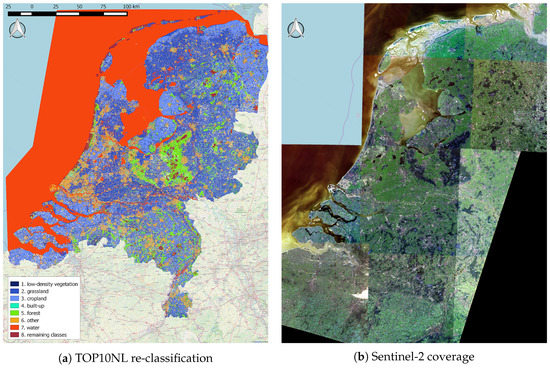
Figure 1.
The re-classified (eight classes) rasterized version of the TOP10NL data set (42,508 km, ∼550 M pixels) and the S2-coverage of the whole country of the Netherlands by one of the two Level-2A Sentinel-2 collections.
3.3. Remote Sensing and Computational Approaches
Although the standard definition of image classification in computer vision applications refers to the process of attributing a single label to the entire image, in remote sensing the term classification signifies the assignment of a categorical label to a single pixel, or to a subset/part of the satellite image (localized labelling). In the single-pixel-based approach which we are interested in, adjacent or connected pixels having the same label form agglomerations which correspond partially or completely to actual objects captured on the image. When the target application is the production of thematic maps and land cover layers, these image partitions represent semantic classes, such as “water”, “urban area”, “vegetation”, and “forest”. In practical terms, the satellite image is divided into distinct segments which, according to human interpretation, convey similar content, and for this reason the classification process can equally be called “semantic segmentation”.
Various feature extraction methods have been developed over the years, striving mainly to establish relationships on the distribution of the radiation’s power in space (radiometry, colour), on the statistical measures describing and summarizing pixel neighbourhoods (texture, corners), on the geometrical–topological properties of the pixel agglomerations (shape, size, compactness), and on similarities/differences between adjacent image regions (context). Each method is seeking to exploit associations along the spectral, spatial, and temporal domain, either separately or in combination. Then, classification techniques attempt to model the functional relationship between the feature vectors and the semantic information. Features employed in [17], for instance, include a gray-level co-occurrence matrix, differential morphological profiles, and an urban complexity index. The study in [18] demonstrated that the object-based classifier is a significantly better approach than the classical per-pixel classifiers when extracting urban land cover using high spatial resolution imagery. Support Vector Machines (SVM) and geometrical moments for automatic recognition of man-made objects have been demonstrated in [19]. A multi-layer perceptron and Radial Basis Function Networks have been used for supervised classification [20]. The use of the Random Forest (RF) classifier for land cover classification is explored in [21]. In order to map land covers, the authors in [22] evaluated the potential of multi-temporal Landsat-8 spectral and thermal imageries using an RF classifier. In a similar application, the classification of high spectral, spatial, and temporal resolution satellite image time-series is evaluated by means of RF and SVM [23]. Similarly, the performance of the RF classifier for land cover classification of a complex area has been explored in [24]. The authors in [25] evaluated the time-weighted dynamic time warping method with Sentinel-2 time-series for pixel-based and object-based classifications of various crop types. In [26], the aim was the crop classification using single-date Sentinel-2 imagery, and was performed by RF and SVM. The authors in [27] tested the ability of Sentinel-2 for forest-type mapping with RF in a Mediterranean environment. Similarly, the authors in [28] examined and compared the performances of RF, k-Nearest Neighbour, and SVM for land use/cover classification using Sentinel-2 image data. In the same line, the study in [29] compared and explored the synergistic use of Landsat-8 and Sentinel-2 data in mapping land use and land cover of rural areas, and by using three machine learning algorithms: RF, Stochastic Gradient Boosting, and SVM. In [30], the authors benchmarked nine machine-learning algorithms in terms of training speed and accuracy classification of land-cover classes in a Sentinel-2 data set. The authors in [31] demonstrated how a convolutional neural network can be applied to multispectral orthoimagery and a digital surface model (DSM) of a small city for a full, fast, and accurate per-pixel classification. Finally, in [32], the Symbolic Machine Learning classifier was applied to investigate the added-value of Sentinel-2 data compared to Landsat in the frame of the Global Human Settlement Layer (https://ghsl.jrc.ec.europa.eu/) scope.
The classical processing chain for satellite image classification is depicted in Figure 2. The feature extraction process involves the computation of quantities referring to spectral (band combinations), textural (pixel or neighbourhood statistics), morphological (topological properties), and similarity-based content.
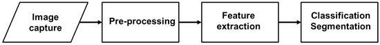
Figure 2.
The classical processing chain for satellite image classification.
As opposed to the traditional pixel-based remote-sensing image classification algorithms in which each single pixel (or pixel vector in the case of images with more than one channel) is individually evaluated [33], in this work we decided to test two computational modelling approaches (convolutional neural networks and random forests) which exploit the contextual information of the pixels and manage to base the classification outcome upon the automatically selected and most discriminative features.
The key characteristics which led us to study and test the specific machine learning techniques are summarized below:
- Both types of modelling are non-parametric and capable of learning any sophisticated mapping;
- They are fast and easy to implement, and can handle a very large number of input variables by keeping the risk of overfitting low;
- Hand-crafted feature extraction is substituted by automatic feature generation, a process in which linear and non-linear mappings are applied to values derived either from the original data or from successive mathematical operations to derivative values; this process takes place while solving the optimization problem which builds the relationships between input and reference data;
- Deep neural networks learn efficiently discriminative features through their natural hierarchical structure; in a similar way, the random forest builds decision trees at which the relationship ancestor/descendant is evaluated based on the discriminative power of the original features;
- Convolutional neural networks maintain an inherent capacity to model complex processes via the use of a high number of parameters (provided that a sufficient number of training data is available, as it is the case with the abundance of Earth observation data). Although the random forest is not so demanding in terms of structural parameters, it has been repeatedly proven to be quite efficient to model complex relationships, mainly due to its streamlined weighting of contributing factors and its effective synthesis of the output provided by ensemble modelling.
Hence, we think that both modelling approaches can adequately address most of the challenges already mentioned in Section 1.
3.3.1. Convolutional Neural Networks
Convolutional Neural Networks (CNN) are models which, by design, exhibit the capacity to represent hierarchically structured data. As the standard neural networks, they consist of a series of layers at which the constituent nodes (computational units) are mathematical functions (linear and/or non linear) which transform the input (weighted combinations of features) they received by the nodes of the previous layer and provide it as input to the next layer. In addition, CNNs are capable of learning local features—that is, a set of weights and biases are applied successively over small subsets of the image. In that way, contextual information that exists in the different areas of the image can be captured, and the most salient features inside the pixel neighbourhoods can be identified. This process is called convolution, and a specific combination of weights with a bias is called the filter [34]. Hyper-parameters at this level are the filter size, the stride which determines the movement pace of the filter over the image, and the mathematical function which translates, point-wise, the outcome of the convolution. CNN can learn features in several abstract layers through non-linear functions, named pooling or sub-sampling operators [35]. Their objective is two-fold: to confer local translational invariance on the already extracted features, and to reduce the computational cost by making the image resolution coarser. Likewise, the mathematical function that defines the pooling operator, the size of the spatial domain at which pooling has effect, and its stride define the hyper-parameters of this pooling layer.
The flexibility to build neural networks by applying different combinations of layers, nodes, operators, ways of connectivity among the computational units, and numerous other parameters provide the great capacity to model complex phenomena and processes at diverse levels of sophistication. Another major attribute is the so-called plasticity [36], the fact that specific computational units across the network layers fire together. In supervised learning, the standard method to properly weigh the node connections is back-propagation [37]. Particularly, the main advantage of CNNs is that the entire system is trained end-to-end, from raw pixels to ultimate categories, thereby alleviating the requirement to manually design a suitable feature extractor [38]. The main disadvantage is the necessity for a considerable number of high-quality labelled training samples due to the large number of parameters to be estimated.
In this work, we experimented with four CNN variants for end-to-end, pixel-to-pixel image segmentation:
- Standard CNN: a network configuration consisting of a sequence of convolutional/pooling layers, which receives as input the neighbourhood (for instance, , or ) of the pixel of interest. At the final layer, the class label of the central pixel of this neighbourhood is predicted;
- Fully Convolutional Network (FCN): the network consists of convolutional/pooling layers only. The final layer performs an upsampling operation to reach the input spatial resolution [39];
- U-net: An extension of the FCN architecture where, among the successive layers of the standard contracting network, the pooling operators have been replaced by upsampling operators, thus increasing the resolution of the output. It has been shown experimentally that the model parameters converge to satisfying estimations with very few training samples [40].
- SegNet: The model is a special case of auto-encoder [41], and has a symmetrical architecture consisting of non-linear processing encoders and decoders followed by a pixel-wise classifier [42].
Figure 3 shows the four basic CNN variants tested in this work. Each network layer is described by the shape of the array it handles, the number of parameters to be estimated, and the mathematical operation that has produced the array. In total, eight building blocks (layers) have been employed to compose the networks: (1) input: the array/tensor which enters the network; (2) 2Dconv: spatial convolution kernels that are convolved with the layer input; (3) batchNorm: normalization of the activations of the previous layer at each batch; the layer is the one defined in [43] where a transformation that maintains the mean activation close to 0 and the activation standard deviation close to 1 is applied.; (4) dense: a densely-connected layer; (5) 2DMaxpool: application of the maximum operator over spatial data; (6) 2DMaxUnpool: upsampling of the layer input by inverting the 2DMaxpool operation; (7) 2DUpsampling: upsampling of the layer input according to a factor applied in rows and columns of the input array, and then interpolation; (8) concat: concatenation of a list of input arrays. Each layer is connected, with the next one, via a black arrow, showing the direction of the coupling. A thicker orange arrow signifies the connection of two layers, where the output array of the first layer has been upsampled appropriately to match the spatial resolution of the array that the second layer accepts as input.
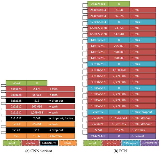
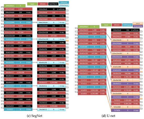
Figure 3.
The four CNN variants tested in this study. Each network layer is described by the shape of the array it handles, the number of parameters to be estimated, and the mathematical operation that has produced the array. In total, eight building blocks (layers) are employed to compose the networks: input, 2Dconv, batchNorm, dense, 2DMaxpool, 2DMaxUnpool, 2DUpsampling, and concat. Each layer is connected with the next one via a black arrow showing the direction of the coupling. A thicker orange arrow signifies the connection of two layers where the output array of the first layer has been upsampled appropriately to match the spatial resolution of the array that the second layer accepts as input.
The spatial size or of the input array is indicative, since we experimented with other array shapes as well, like , and . The number of rows and columns of the input and the output array for the FCN, SegNet, and U-net networks is the same; only the third (channel) dimension differs, being 4 matrices as input, 8 matrices as output. The fourth CNN variant takes as input a 3D-array and returns as output an 8-element vector (each of the 8 values corresponding to one of the 8 classes). Consequently, in order to achieve end-to-end image segmentation by using those CNN models, the user needs to either cut the satellite image in blocks of specific size in the case of FCN, SegNet, and U-net, or to generate blocks following a sliding window approach in the case of the standard CNN variant.
3.3.2. Random Forest Classifier
Random Forests (RF) is a machine-learning method dealing mostly with classification and regression problems (supervised learning), but also with unsupervised learning and feature evaluation tasks. It is based on the concept of ensemble modelling—that is, a certain number of decision trees acting as base models is growing and the optimal configuration is chosen depending on the synthesis and aggregation of the individual results and the final predictive accuracy. Herein, we employ the bagging approach [44] introduced by [45] that combines bootstrapping and aggregation to form the ensemble model. The generalization error of a forest of tree classifiers depends on the capacity of the individual trees in the forest and the correlation between them. Selecting a random subset of features at each candidate split during the learning process minimizes the correlation among the classifiers in the ensemble, eliminates the necessity for branch pruning (contrary to the classical decision trees), and yields progressively lower error rates.
A new feature vector is classified by each of the trees in the forest. Even if the time complexity of RF is a function of the number of base trees, the prediction response of the ensemble proves to be considerably fast. Each tree provides a classification outcome and the forest decision accounts the majority of the votes over all the trees in the forest.
4. Results
One of the objectives of this study was to evaluate how some basic hyper-parameters and the amount of training samples impact the classification accuracy. Furthermore, dimensions like training/prediction time, as well as model robustness on different input signals have been taken into account. Analytically, we elaborated and assessed the following factors:
- Number of training samples: a high number of model parameters requires an even bigger number of training samples (model complexity), especially when the problem at hand is a multi-class classification (problem complexity);
- Transfer learning: intentionally, we did not make use of pre-trained layers so as to check the capacity of the models to extract discriminative features from the input imagery and also to measure the actual training time. However, we adopted another version of transfer learning by assessing the model performance either on a different type of input imagery (S2 processing levels), or against disparate reference data;
- Hyper-parameters: since the models under consideration are multi-parametric, it is practically impossible to quantify the effect of all the model parameters in an exhaustive way. As it is described in the following sections, we selected the parameters which, in our opinion, play a critical role on the model performance. Parameters such as the window size of the convolution or pooling layers, and the window stride in the case of CNNs, or the minimum number of samples required to exist at a leaf node, and the minimum number of samples required to split an internal node in respect of RF did not have a variable value in our experiments. Such parameters certainly affect the model performance, but we consider them as having the potential to improve the fine-tuning of the model.
4.1. Pre-Processing and Data Handling
The input imagery from both L1C and L2A products are the 10 m spectral bands. For L1C, the physical values (Top of the Atmosphere normalized reflectances) have been coded as integers on 15 bits, and range from 1 (minimum reflectance ) to 10,000 (reflectance 1); values higher than 1 can be observed in some cases due to specific angular reflectivity effects. The special value 0 signifies “no data”. Regarding L2A, the surface reflectance values are coded with the same quantification value of 10,000 as for L1C products [46]. For this reason, we have applied a factor of 1/10,000 to retrieve physical reflectance values. In addition, we standardized the data through the z-transform by subtracting the average value and dividing by the standard deviation in each band. The parameters of the transformation were always estimated from the training set under consideration; then, the same z-transform was applied on the respective testing data. To avoid confusion between the valid 0 values and the “no data” values, a separate binary mask D was produced before the application of the z-transform.
A stratified sampling was adopted for the samples selection, attempting to keep a constant percentage for every class. The original reference set is highly imbalanced in favour of the classes “grassland” and “water”, while on the opposite side, the classes “built-up” and “low-density vegetation” are under-represented (Table 1).
4.2. Training Phase
During the training phase, a fraction of 0.1 of the training data was reserved for validation in order for the CNNs to prevent over-fitting. The number of epochs to train the models were defined to 100 iterations. The weights were initialized based on uniform distribution with bounds . We tested two loss functions: the dice loss
and the categorical cross-entropy
where C is the set of classes, N is the set of the pixels used for the training, is the matrix of the real target values of the training set in binary coding, and is the matrix of the model responses in the continuous range . We avoided using loss weighting so that we could measure the effect of class imbalance. The early stopping of the training was activated—that is, training terminates when the chosen loss function stops improving. In regard to the activation functions, we tested the standard rectifier function, the hyperbolic tangent function, and the logistic sigmoid function, respectively:
In the last layer, we employed the softmax function:
having (cardinality of the set C) denoting the number of classes. For the optimization part, the Adaptive Moment Estimation method (Adam) was chosen, an algorithm for first-order, gradient-based optimization of stochastic objective functions based on adaptive estimates of lower-order moments [47]. Since the model training takes place on a Graphical Processing Unit, the memory of which does not fit in the amount of training data, the learning occurs in a batch-wise fashion. The size of each mini-batch is variant, and depends on the model topology and the respective parameters.
To avoid overfitting, RF was adjusted using stratified two-fold cross-validation combined with a randomized search on the hyper-parameters domain. We focused mainly on the following parameters: number of trees that compose the forest, the depth of the tree, and the number of features that are considered when seeking the best split. To reduce, in reasonable levels, the computational cost of the hyper-parameters optimization, we fixed the number of parameter settings that were sampled to 12 trials. The locally optimal cut-point for each feature was computed based on either the information gain (the expected amount of information that would be needed to specify whether a new instance should be classified in one of the categories, given that the example reached that node [48]) or the Gini impurity [49].
4.3. Evaluation Metrics
Four metrics were used to assess the accuracy and precision of the classification results: (1) Overall Accuracy:
where input corresponds to the valid pixels that compose the valid data domain of the testing set (Section 4.1), is the vector of the real target values of the testing set, and is the vector of the model responses. stands for true positive, for true negative, for false positive and for false negative, respectively. The overall accuracy metric reflects the actual accuracy when the target classes are nearly balanced; yet, we provide this metric for reference and cross-comparison reasons; (2) F1-score (macro):
where , and ; this metric works preferably with uneven class distributions because it better balances a poor precision with an excessive recall; (3) Weighted Accuracy:
where is the number of classes, is the total number of valid values, and is the number of valid values with respect to class c; (4) F1-score (weighted):
The last two metrics take into consideration the amount of true instances for each class label (support); hence, they highlight the deeper contribution of each class that is proportional to its size. All the metrics hold that the better the classification results, the closer the metric values are to 1.
In addition, we provide confusion matrices for several models in order for the reader to better understand the omission and commission errors produced by each of the presented model configurations.
4.4. Performance Figures
Table 3 summarizes the experimental results. The meaning of the column headers is described below:
Table 3.
Indicative experimental results in terms of classification performance metrics and training/prediction time. Highest scores have been emphasized in bold type.
- Model: The symbolic name “M-L-L-W” of the computational model. The notation is explained as follows: (i) M refers to the classifier type, i.e., RF, CNN, FCN, Unet, or SegNet; (ii) L denotes one of the four groups of the S2 products: L1C(winter), L2A(winter), L1C(spring), L2A(spring); (iii) The first L points at the series of products used for training, and the second L at the products used for testing purposes. When the letter L appears in both positions, it means firstly that the group of products for training and testing is the same, and secondly that the classification results are similar in any of the four cases; also, notation like L1Cmix signifies L1C image blocks taken from both winter and spring seasons; (iv) W signifies the size of the spatial window. Especially for the cases of RF and standard CNN, it means: Input: pixels per band; Output: one class label corresponding to the central input pixel of the spatial window ;
- Training time: the elapsed time in seconds for processing 1M training samples (pixels) and with respect to the number of processing units described in Section 4.5 (hardware specs);
- Prediction time: the elapsed time in seconds for processing 1M testing samples (pixels) and with respect to the number of processing units described in Section 4.5 (hardware specs);
- OA: Overall Accuracy (range [0, 1], best value 1);
- WA: Weighted Accuracy (range [0, 1], best value 1);
- F1-macro: F1-score (macro) (range [0, 1], best value 1);
- F1-weighted: F1-score (weighted) (range [0, 1], best value 1).
The mean ± standard deviation are shown in regard to both training and prediction time, and any of the four classification metrics. The results refer to five repetitions for every different model configuration. For instance, for a CNN model tested with three spatial window sizes, 16 options for training and testing in regard to the S2 products, 12 network topologies by five repetitions results in 2880 trials.
Figure 4 demonstrates the impact of the training set size on the classification efficiency when measured on the testing set. The weighted F1-score represents the median values after considering all model configurations that we tested. As expected, the F1-score improves as the size of the training set becomes larger, and after a certain point for every model it starts to saturate. In the case of RF, saturation happens quickly and with a much smaller training set. We noticed that the specific RF implementation (see Section 4.5) can efficiently handle a high number of training samples. This number depends on the parameter settings and the memory resources of the hardware; in our tests, this number could not surpass a certain order of magnitude.
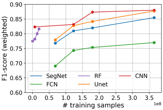
Figure 4.
Effect of the training-set size on the weighted F1-score.
Table 4 and Table 5 present joint confusion matrices for selected models that cover the most of the cases and provide a clear picture regarding the plurality of the results that have been produced. The numbers which appear in the second column correspond to the models at the bottom of the tables. The highest percentage for each pair of classes has been emphasized in bold type.
Table 4.
Confusion matrix for selected models.
Table 5.
Confusion matrix for selected models.
Figure 5 displays the full confusion matrix of one of the most performant modelling approaches, the training of which was based on two different seasons (early winter and late spring). It summarizes the classification results produced by the not-so-complex model (1,449,352 parameters) CNN-L1Cmix-L1Cmix-5x5.
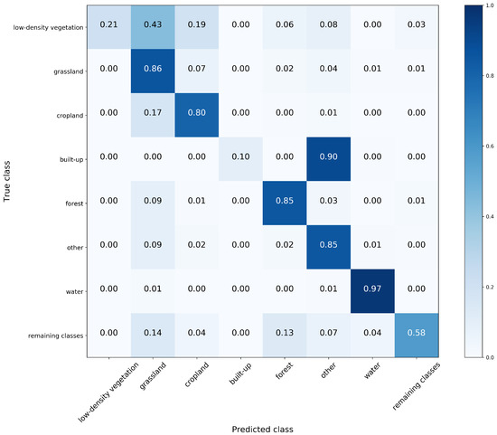
Figure 5.
Confusion matrix referring to the model CNN-L1Cmix-L1Cmix-5x5.
The following illustrations (Figure 6, Figure 7 and Figure 8) depict some representative results from six different locations spread over the Netherlands. They are structured in groups of two columns. Reading from left to right in each of the six groups, the first row contains the RGB composition of the input image and the respective re-classified eight-classes map based on the TOP10NL layer. The second row displays the classification outcome of one instance of the single-season models RF-L1C-1x1 and RF-L2A-3x3, while the third row the outcome of RF-L1C-5x5 and the one of the simple SegNet-L1C-244x244. Next, the fourth row shows the output of FCN-L1C-244x244 and SegNet-L1Cmix-244x244, the fifth row the output of Unet-L1Cmix-244x244 and Unet-L1C(winter)-244x244, and finally the sixth row shows the output of CNN-L1Cmix-5x5 and CNN-L1C(winter)-5x5, respectively.
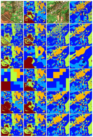
Figure 6.
Indicative classification results. Classes: low-density vegetation (dark blue), grassland (blue), cropland (light blue), built-up (blue-green), forest (green), other (orange), water (red), and remaining classes (brown).
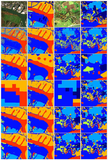
Figure 7.
Indicative classification results. Classes: low-density vegetation (dark blue), grassland (blue), cropland (light blue), built-up (blue-green), forest (green), other (orange), water (red), and remaining classes (brown).
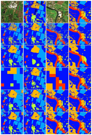
Figure 8.
Indicative classification results. Classes: low-density vegetation (dark blue), grassland (blue), cropland (light blue), built-up (blue-green), forest (green), other (orange), water (red), and remaining classes (brown).
The last experiment is a transfer learning exercise that checks the robustness of the model when applied on different geographic regions. The study area has been chosen to be a division of Albania. The S2 imagery (see Appendix A) used as input is of type L1C and has sensing time stamp 20181113. This exercise actually constitutes a simulation of how possible gaps existing in the INSPIRE data sets could potentially be filled in by automated methods, the configuration of which has been based on the standards and nomenclature of different authorities. As a reference layer, we employed the CORINE (coordination of information on the environment) Land Cover 2018 (https://land.copernicus.eu/pan-european/corine-land-cover/clc2018) product after re-classification to approximately match the classification schema based on the TOP10NL data set. The re-classification of CORINE 2018 (for which we do not claim that is universally defined with the proposed schema) is shown in Table 6. Figure 9 shows some indicative cases from this experiment; the outcome of the three models SegNet-L1Cmix-244x244, Unet-L1Cmix-244x244, and CNN-L1Cmix-5x5 is also included. Although we do not make use of the NDVI, we have included it in this figure in order to show what type of information the standard spectral-based features convey and also to help the reader to easily identify the green areas as well as the water bodies in the opposite side of the range. The approximate accordance between the output and the reference layer has been confirmed visually after qualitative analysis.
Table 6.
Re-classification of the CORINE Land Cover 2018 data set according to the TOP10NL-based reference layer.
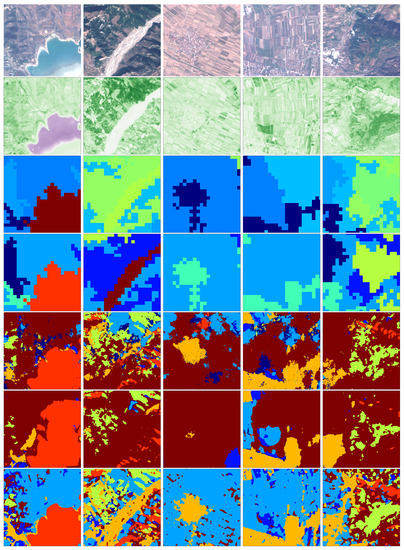
Figure 9.
Checking the model robustness. Area of study: Albania. Reference layer: CORINE 2018 re-classified. Rows: (1) RGB composition of the input S2 imagery; (2) NDVI; (3) CORINE 2018; (4) CORINE 2018 re-classified; (5) SegNet-L1Cmix-244x244; (6) Unet-L1Cmix-244x244; (7) CNN-L1Cmix-5x5. The NDVI colormap ranges from value -1 (purple) to value 0 (white) and then to value 1 (dark green). The CORINE 2018 discrete colormap represents the respective classes shown in Table 6, 3rd column, as being ordinal values. The re-classified CORINE 2018 colormap as well as the colormap of the depicted models output follows the colour convention defined in Table 6, 1st and 2nd column.
4.5. The Computational Platform: JRC Earth Observation Data and Processing Platform (JEODPP)
Sensitivity analysis of complex models through the exploration of various hypotheses defined by different parametrizations, together with the models training which is based on big amounts of data, constitutes a challenging task and invites unconventional computational capacity. CNNs rely heavily on matrix mathematical operations, and their inherent multi-layered architecture requires tremendous amounts of floating-point computations. Naturally, this is something that can be done in parallel mode and especially by exploiting the capacity of Graphical Processing Units. Likewise, Random Forests are growing numerous tree classifiers in a parallel fashion, and consequently, their performance is boosted when executing over multi-processing unit configurations.
Cloud working environments (e.g., Google Earth Engine, Amazon Web Services) are platforms that provide lots of open Earth observation data and where the user can efficiently prototype and parallelize her workflows. Alongside these developments, the Copernicus cloud-based infrastructure Data and Information Access Services Operations-DIAS (https://www.copernicus.eu/en/access-data/dias) is progressively undertaking its prescribed operational role. Despite the availability of such computational resources and data, the workflow escalation and the broad-range hypotheses exploration are not straightforward and frequently do not come without cost.
The Joint Research Centre of the European Commission has recently developed a versatile multi-petabyte scale platform based on storage co-located with a high-throughput computing capacity, the so-called JRC Earth Observation Data and Processing Platform (JEODPP) [50]. The platform (https://cidportal.jrc.ec.europa.eu/home/) has been built upon the near-data processing concept which prescribes the computing facility to be placed close to the storage units in order to resolve the bottleneck of delaying or degrading interconnection. The JEODPP provides a great number of CPU and GPU-based processing nodes. For the exercise under consideration, the CNNs training has been performed on Tesla K80 GPUs (Kepler GPU architecture; 4992 NVIDIA CUDA cores with a dual-GPU design; GB of GDDR5 memory; up to 8.73 teraflops single-precision performance with NVIDIA GPU Boost), whereas the RFs training over CPU-based processing nodes respectively (Intel(R) Xeon(R) CPU E5-2698 v4 @ 2.20 GHz; RAM 512GB DIMM DDR4 Synchronous Registered (Buffered) 2400 MHz; 40 processors (20 CPU cores each); cache size 51,200 KB each processor). Apart from the hardware configuration, the performance is highly dependent on the used software and the efficient algorithmic implementations it supports. The JEODPP accommodates and promotes open source implementations, especially in the Python programming language. For the experiments demonstrated in this work the following Python packages have been employed: TensorFlowTM as back-end (https://www.tensorflow.org/) and Keras (https://keras.io/) as front-end for the CNN tests and scikit-learn (https://scikit-learn.org/stable/) for the RF implementations. Analysis and prototyping has been carried out via Jupyter (https://jupyter.org/) notebooks. All the trained models are accessible through the JEODPP and can be made available upon request.
5. Discussion
The findings of the experimental analysis have been consolidated in the following points:
- The results confirmed the high modelling capacity of both RFs and CNN variants for end-to-end S2 image segmentation, a fact that agrees with the until now experimental evidence stating that such kind of models are general-purpose accurate learning techniques;
- Basic hyper-parameters of both approaches do not affect the classification performance so much, exhibiting a high level of stability given the existence of adequate number of training data. The categorical entropy loss function in the CNN case and the Gini impurity in the RF case slightly lead to better results. For the deep models Unet, SegNet, and FCN, the rectifier function reduced the computational cost a lot and resulted in better classification, whereas in the case of the less deep topologies of the CNN-wxw models, the hyperbolic tangent as activation function was proven more effective;
- Similarly, the processing level of S2 products (either L1C or L2A) does not have a significant impact on the classification results;
- On the contrary, variability due to different seasonal conditions can only be captured by introducing training samples referring to different sensing time stamps. Analysis and modelling of time-series turns to be key component for such type of tasks. CNNs appear more robust and capture better the data variability (landscape diversity and variable time) and it is due to the high number of parameters they come with;
- In the case of Unet, SegNet, and FCN networks, the spatial size of the input tensor has an impact on the classification results. In lower sizes, a more complex architecture (using a high number of filters) is required, whereas in greater sizes there is a strong need for an increasing number of training samples. For the exercise presented herein, a spatial size of 244 × 244 is near to optimal;
- The built-up class cannot be modelled easily due to the inherent mapping issues already mentioned in Section 3.1. It is confused with the class other. In addition, this happens because of the strong overlapping of the two signal signatures and due to the shortage of training samples pointing at the class built-up. The same phenomenon occurs with the class low-density vegetation and the classes grassland and cropland, especially in the spring season. However, we noticed some exceptional cases like the RF-1x1 which confuses grassland and remaining classes but detects sufficiently the built-up class. In reality, when the class is represented by a high number of training samples as it is the case of water, any type of the tested modelling approaches is proven efficient;
- Pixel mismatching between the model output and the reference layer is sometimes due to the fact that the model response is based on the S2 input and its sensing conditions. Actually, the model output can be seen as an updated version of the reference layer, where there is a trade-off among the properties of both the input and reference layers;
- The simple SegNet approach returns as response a rather coarse segmentation. In a similar way, FCN gives an output having the block effect. Both network configurations require more and finer upsampling layers contracting somehow with the downsampling layers, as it happens in the architectures of Unet and SegNet. This is also evidence that from one side, a deep neural network has the flexibility to model complex problems but from the other side, it requires tedious and long-lasting fine-tuning in order to draw an optimal configuration for the task at hand;
- In most of the cases, RF performs quite well even if it does not make use of the feature localization attribute provided by the convolutional filters. In order to capture the high variability existing in the samples, RF tends to grow long trees, a fact which may lead to overfitting. Keeping shorter the size of the trees results sometimes in a weak modelling. In conclusion, RF inherent capacity has an upper bound that puts a ceiling on the modelling of complex processes.
- The results from the transfer learning exercise show an acceptable level of classification agreement given the geographical and morphological discrepancies of the two countries (Netherlands and Albania). Nevertheless, when the target application is a European land cover map, the exploitation of additional information sources and databases like the BigEarthNet [51] or Corine Land Cover 2018 is imperative;
- For big training sets, CPU or GPU-based parallelization is necessary for both CNNs and RFs; the prediction time remains in a sufficient level. The former fact confirms the need for specialized computational resources and dedicated Earth Observation exploitation platforms. With this work, we demonstrate that JEODPP, the EC JRC high-throughput and high-performance computational platform that is gradually being built, is evolving in the proper direction.
Among the CNN variants, we found the CNN-5x5 model (especially the one trained on samples from both winter and spring seasons) quite performant given the relatively low architecture complexity and robust enough to varying conditions.
6. Conclusions
Satellite missions compliant with the open and free data distribution regime like Sentinel and Landsat continuously acquire data and compose satellite image time-series which serve in a plethora of applications, such as environmental management and monitoring, climate change, agriculture, urban planning, biodiversity conservation, and land change detection, to mention some. Human-based analysis of large areas and manual inspection of multiple images have been proven costly and time consuming. The emergence of machine learning facilitates the automation of Earth observation analysis, helps to uncover complex spatio-temporal patterns and results in insightful and profound understanding of the physical processes.
Working in the machine learning framework, this paper demonstrates the modelling capacity of two state-of-the-art classifiers, the Convolutional Neural Networks and the Random Forests, whilst tackling the multi-class, “end-to-end”, 10 m Sentinel-2 image segmentation. The class annotations have been derived from a re-classified layer based on the Dutch country-level data set made available in the INSPIRE infrastructure. Extensive performance and sensitivity analysis of the most significant hyper-parameters demonstrates a quite stabilized performance. The classification results can be considered satisfactory for such kind of exercise, and confirm in a positive way the high performance of those classifiers, a finding that remote sensing studies gradually verify. Furthermore, the proposed approach illustrates the potential of combining open data from multiple sources for the acquisition of new knowledge. From the perspective of spatial data infrastructures the benefits are manifold: (i) generation of new data with high spatial and temporal resolution, (ii) ability to use Sentinel data for different geographic regions where other data sets are not available, and (iii) possibility for quality validation and updating of the input (e.g., INSPIRE) data.
Keeping the current study as baseline, the next step is to elaborate the production of an European land cover based on the continuous acquisition of Earth observation data provided by the Copernicus Sentinel missions and particularly by the Sentinel-1 and Sentinel-2 satellites. With orbits repeating every six days for the former and five days for the latter, large swath, and rich spectral and spatial resolution, these two sensors enable the utilization of satellite image time-series which constitute necessary component for land cover change detection and land-use monitoring.
Author Contributions
B.D. and A.K. conceived the idea of combining INSPIRE data with the U-net and Random Forest models and produced preliminary results on a small-scale data set; V.S., P.H., P.K. and P.S. expanded the study on the whole country of Netherlands, by using various types of Sentinel-2 products and by testing multiple models based on convolutional neural network and Random Forest approaches; V.S. designed and implemented the experimental study; V.S. wrote the paper and all the authors reviewed and edited it.
Funding
This research received no external funding.
Acknowledgments
The authors would like to thank Tomáš Kliment for his contribution in selecting and downloading the Sentinel-2 products and the JEODPP team operating the platform.
Conflicts of Interest
The authors declare no conflict of interest.
Appendix A
The list of Sentinel-2 products used as input imagery to the computational models:
Level-1C, sensing time: early winter
- S2B_MSIL1C_20181010T104019_N0206_R008_T32ULC_20181010T161145.SAFE
- S2B_MSIL1C_20181010T104019_N0206_R008_T31UGU_20181010T161145.SAFE
- S2A_MSIL1C_20181117T105321_N0207_R051_T31UET_20181117T112412.SAFE
- S2A_MSIL1C_20181117T105321_N0207_R051_T31UFU_20181117T112412.SAFE
- S2A_MSIL1C_20181117T105321_N0207_R051_T31UFS_20181117T112412.SAFE
- S2A_MSIL1C_20181117T105321_N0207_R051_T31UFT_20181117T112412.SAFE
- S2A_MSIL1C_20181117T105321_N0207_R051_T31UGS_20181117T112412.SAFE
- S2A_MSIL1C_20181117T105321_N0207_R051_T31UFV_20181117T112412.SAFE
- S2B_MSIL1C_20181212T105439_N0207_R051_T31UES_20181212T112608.SAFE
- S2A_MSIL1C_20181117T105321_N0207_R051_T31UGV_20181117T112412.SAFE
- S2A_MSIL1C_20181117T105321_N0207_R051_T31UGT_20181117T112412.SAFE
Level-2A, sensing time: early winter
- S2B_MSIL2A_20181010T104019_N0209_R008_T32ULC_20181010T171128.SAFE
- S2B_MSIL2A_20181010T104019_N0209_R008_T31UGU_20181010T171128.SAFE
- S2A_MSIL2A_20181117T105321_N0210_R051_T31UET_20181117T121932.SAFE
- S2A_MSIL2A_20181117T105321_N0210_R051_T31UFU_20181117T121932.SAFE
- S2A_MSIL2A_20181117T105321_N0210_R051_T31UFS_20181117T121932.SAFE
- S2A_MSIL2A_20181117T105321_N0210_R051_T31UFT_20181117T121932.SAFE
- S2A_MSIL2A_20181117T105321_N0210_R051_T31UGS_20181117T121932.SAFE
- S2A_MSIL2A_20181117T105321_N0210_R051_T31UFV_20181117T121932.SAFE
- S2B_MSIL2A_20181212T105439_N0211_R051_T31UES_20181218T134549.SAFE
- S2A_MSIL2A_20181117T105321_N0210_R051_T31UGV_20181117T121932.SAFE
- S2A_MSIL2A_20181117T105321_N0210_R051_T31UGT_20181117T121932.SAFE
Level-1C, sensing time: late spring
- S2A_MSIL1C_20180508T104031_N0206_R008_T32ULD_20180508T175127.SAFE
- S2A_MSIL1C_20180508T104031_N0206_R008_T31UGS_20180508T175127.SAFE
- S2A_MSIL1C_20180508T104031_N0206_R008_T32ULC_20180508T175127.SAFE
- S2A_MSIL1C_20180508T104031_N0206_R008_T32ULE_20180508T175127.SAFE
- S2A_MSIL1C_20180508T104031_N0206_R008_T31UFS_20180508T175127.SAFE
- S2B_MSIL1C_20180506T105029_N0206_R051_T31UET_20180509T155709.SAFE
- S2B_MSIL1C_20180506T105029_N0206_R051_T31UFT_20180509T155709.SAFE
- S2B_MSIL1C_20180506T105029_N0206_R051_T31UFU_20180509T155709.SAFE
- S2B_MSIL1C_20180506T105029_N0206_R051_T31UES_20180509T155709.SAFE
- S2B_MSIL1C_20180506T105029_N0206_R051_T31UFV_20180509T155709.SAFE
- S2B_MSIL1C_20180506T105029_N0206_R051_T31UGT_20180509T155709.SAFE
Level-2A, sensing time: late spring
- S2A_MSIL2A_20180508T104031_N0207_R008_T32ULD_20180508T175127.SAFE
- S2A_MSIL2A_20180508T104031_N0207_R008_T31UGS_20180508T175127.SAFE
- S2A_MSIL2A_20180508T104031_N0207_R008_T32ULC_20180508T175127.SAFE
- S2A_MSIL2A_20180508T104031_N0207_R008_T32ULE_20180508T175127.SAFE
- S2A_MSIL2A_20180508T104031_N0207_R008_T31UFS_20180508T175127.SAFE
- S2B_MSIL2A_20180506T105029_N0207_R051_T31UET_20180509T155709.SAFE
- S2B_MSIL2A_20180506T105029_N0207_R051_T31UFT_20180509T155709.SAFE
- S2B_MSIL2A_20180506T105029_N0207_R051_T31UFU_20180509T155709.SAFE
- S2B_MSIL2A_20180506T105029_N0207_R051_T31UES_20180509T155709.SAFE
- S2B_MSIL2A_20180506T105029_N0207_R051_T31UFV_20180509T155709.SAFE
- S2B_MSIL2A_20180506T105029_N0207_R051_T31UGT_20180509T155709.SAFE
The L1C Sentinel-2 product used to test the robustness of the computational models (in combination with the CORINE Land Cover 2018):
- S2A_MSIL1C_20181113T093231_N0207_R136_T34TDL_20181113T100054.SAFE
References
- Treitz, P. Remote sensing for mapping and monitoring land-cover and land-use change. Prog. Plan. 2004, 61, 267. [Google Scholar] [CrossRef]
- Drusch, M.; Bello, U.D.; Carlier, S.; Colin, O.; Fernandez, V.; Gascon, F.; Hoersch, B.; Isola, C.; Laberinti, P.; Martimort, P.; et al. Sentinel-2: ESA’s Optical High-Resolution Mission for GMES Operational Services. Remote Sens. Environ. 2012, 120, 25–36. [Google Scholar] [CrossRef]
- Lu, D.; Weng, Q. A Survey of Image Classification Methods and Techniques for Improving Classification Performance. Int. J. Remote Sens. 2007, 28, 823–870. [Google Scholar] [CrossRef]
- Ball, J.; Anderson, D.; Chan, C.S. A Comprehensive Survey of Deep Learning in Remote Sensing: Theories, Tools and Challenges for the Community. J. Appl. Remote Sens. 2017, 11, 042609. [Google Scholar] [CrossRef]
- Camps-Valls, G.; Tuia, D.; Bruzzone, L.; Benediktsson, J.A. Advances in Hyperspectral Image Classification: Earth Monitoring with Statistical Learning Methods. IEEE Signal Process. Mag. 2014, 31, 45–54. [Google Scholar] [CrossRef]
- Noh, H.; Hong, S.; Han, B. Learning Deconvolution Network for Semantic Segmentation. In Proceedings of the 2015 IEEE International Conference on Computer Vision (ICCV ’15), 7–13 December 2015; IEEE Computer Society: Washington, DC, USA, 2015; pp. 1520–1528. [Google Scholar] [CrossRef]
- Bischke, B.; Helber, P.; Folz, J.; Borth, D.; Dengel, A. Multi-Task Learning for Segmentation of Building Footprints with Deep Neural Networks. arXiv, 2017; arXiv:1709.05932. [Google Scholar]
- Zhu, X.X.; Tuia, D.; Mou, L.; Xia, G.; Zhang, L.; Xu, F.; Fraundorfer, F. Deep Learning in Remote Sensing: A Comprehensive Review and List of Resources. IEEE Geosci. Remote Sens. Mag. 2017, 5, 8–36. [Google Scholar] [CrossRef]
- Circular No. A-16 Revised. Available online: https://obamawhitehouse.archives.gov/omb/circulars_a016_rev/#2 (accessed on 2 October 2019).
- Craglia, M.; Annoni, A. INSPIRE: An innovative approach to the development of spatial data infrastructures in Europe. In Research and Theory in Advancing Spatial Data Infrastructure Concepts; ESRI Press: Readland, CA, USA, 2007; pp. 93–105. [Google Scholar]
- Williamson, I.; Rajabifard, A.; Binns, A. The role of Spatial Data Infrastructures in establishing an enabling platform for decision making in Australia. In Research and Theory in Advancing Spatial Data Infrastructure Concepts; ESRI Press: Readland, CA, USA, 2007; pp. 121–132. [Google Scholar]
- The Global Monitoring for Environment and Security (GMES) Programme. Available online: https://www.esa.int/About_Us/Ministerial_Council_2012/Global_Monitoring_for_Environment_and_Security_GMES (accessed on 10 February 2019).
- Stoter, J.; van Smaalen, J.; Bakker, N.; Hardy, P. Specifying Map Requirements for Automated Generalization of Topographic Data. Cartogr. J. 2009, 46, 214–227. [Google Scholar] [CrossRef]
- The INSPIRE TOP10NL. Available online: https://www.pdok.nl/downloads?articleid=1976855 (accessed on 10 February 2019).
- GDAL/OGR Contributors. GDAL/OGR Geospatial Data Abstraction Software Library. Open Source Geospatial Foundation. Available online: http://gdal.org (accessed on 10 February 2019).
- Sentinel-2 Products Specification Document. Available online: https://sentinels.copernicus.eu/documents/247904/685211/Sentinel-2-Products-Specification-Document (accessed on 10 February 2019).
- Huang, X.; Zhang, L. An SVM Ensemble Approach Combining Spectral, Structural, and Semantic Features for the Classification of High-Resolution Remotely Sensed Imagery. IEEE Trans. Geosci. Remote Sens. 2013, 51, 257–272. [Google Scholar] [CrossRef]
- Myint, S.W.; Gober, P.; Brazel, A.; Grossman-Clarke, S.; Weng, Q. Per-pixel vs. object-based classification of urban land cover extraction using high spatial resolution imagery. Remote Sens. Environ. 2011, 115, 1145–1161. [Google Scholar] [CrossRef]
- Inglada, J. Automatic recognition of man-made objects in high resolution optical remote sensing images by SVM classification of geometric image features. ISPRS J. Photogramm. Remote Sens. 2007, 62, 236–248. [Google Scholar] [CrossRef]
- Foody, G. Supervised image classification by MLP and RBF neural networks with and without an exhaustively defined set of classes. Int. J. Remote Sens. 2004, 25, 3091–3104. [Google Scholar] [CrossRef]
- Oskar Gislason, P.; Benediktsson, J.; Sveinsson, J. Random Forests for land cover classification. Pattern Recognit. Lett. 2003, 27, 294–300. [Google Scholar] [CrossRef]
- Eisavi, V.; Homayouni, S.; Yazdi, A.M.; Alimohammadi, A. Land cover mapping based on random forest classification of multitemporal spectral and thermal images. Environ. Monit. Assess. 2015, 187, 291. [Google Scholar] [CrossRef] [PubMed]
- Pelletier, C.; Valero, S.; Inglada, J.; Champion, N.; Dedieu, G. Assessing the robustness of Random Forests to map land cover with high resolution satellite image time series over large areas. Remote Sens. Environ. 2016, 187, 156–168. [Google Scholar] [CrossRef]
- Rodriguez-Galiano, V.; Ghimire, B.; Rogan, J.; Chica-Olmo, M.; Rigol-Sanchez, J. An assessment of the effectiveness of a random forest classifier for land-cover classification. ISPRS J. Photogramm. Remote Sens. 2012, 67, 93–104. [Google Scholar] [CrossRef]
- Belgiu, M.; Csillik, O. Sentinel-2 cropland mapping using pixel-based and object-based time-weighted dynamic time warping analysis. Remote Sens. Environ. 2018, 204, 509–523. [Google Scholar] [CrossRef]
- Saini, R.; Ghosh, S.K. Crop Classification on Single Date Sentinel-2 Imagery Using Random Forest and Suppor Vector Machine. Int. Arch. Photogramm. Remote Sens. Spat. Inf. Sci. 2018, XLII-5, 683–688. [Google Scholar] [CrossRef]
- Puletti, N.; Chianucci, F.; Castaldi, C. Use of Sentinel-2 for forest classification in Mediterranean environments. Ann. Silvic. Res. 2018, 42, 32–38. [Google Scholar] [CrossRef]
- Phan, T.N.; Kappas, M. Comparison of Random Forest, k-Nearest Neighbor, and Support Vector Machine Classifiers for Land Cover Classification Using Sentinel-2 Imagery. Sensors 2017, 18, 18. [Google Scholar] [CrossRef]
- Forkuor, G.; Dimobe, K.; Serme, I.; Tondoh, J.E. Landsat-8 vs. Sentinel-2: Examining the added value of sentinel-2’s red-edge bands to land-use and land-cover mapping in Burkina Faso. GISci. Remote Sens. 2018, 55, 331–354. [Google Scholar] [CrossRef]
- Pirotti, F.; Sunar, F.; Piragnolo, M. Benchmark of Machine Learning Methods for Classification of A Sentinel-2 Image. Int. Arch. Photogramm. Remote Sens. Spat. Inf. Sci. 2016, XLI-B7, 335–340. [Google Scholar] [CrossRef]
- Längkvist, M.; Kiselev, A.; Alirezaie, M.; Loutfi, A. Classification and Segmentation of Satellite Orthoimagery Using Convolutional Neural Networks. Remote Sens. 2016, 8, 329. [Google Scholar] [CrossRef]
- Pesaresi, M.; Corbane, C.; Julea, A.; Florczyk, A.J.; Syrris, V.; Soille, P. Assessment of the Added-Value of Sentinel-2 for Detecting Built-up Areas. Remote Sens. 2016, 8, 299. [Google Scholar] [CrossRef]
- Lillesand, T.M. Remote Sensing and Image Interpretation; John Wiley & Sons, Inc.: Hoboken, NJ, USA, 2008. [Google Scholar]
- LeCun, Y.; Bengio, Y.; Hinton, G.E. Deep learning. Nature 2015, 521, 436–444. [Google Scholar] [CrossRef]
- Lecun, Y. Generalization and network design strategies. In Connectionism in Perspective; Pfeifer, R., Schreter, Z., Fogelman, F., Steels, L., Eds.; Elsevier: Amsterdam, The Netherlands, 1989. [Google Scholar]
- Haykin, S. Neural Networks: A Comprehensive Foundation, 2nd ed.; Prentice Hall PTR: Upper Saddle River, NJ, USA, 1998. [Google Scholar]
- LeCun, Y.A.; Bottou, L.; Orr, G.B.; Müller, K.R. Efficient BackProp. In Neural Networks: Tricks of the Trade, 2nd ed.; Montavon, G., Orr, G.B., Müller, K.R., Eds.; Springer: Berlin/Heidelberg, Germany, 2012; pp. 9–48. [Google Scholar]
- Lecun, Y.; Bottou, L.; Bengio, Y.; Haffner, P. Gradient-based learning applied to document recognition. Proc. IEEE 1998, 86, 2278–2324. [Google Scholar] [CrossRef]
- Shelhamer, E.; Long, J.; Darrell, T. Fully Convolutional Networks for Semantic Segmentation. IEEE Trans. Pattern Anal. Mach. Intell. 2017, 39, 640–651. [Google Scholar] [CrossRef]
- Ronneberger, O.; Fischer, P.; Brox, T. U-Net: Convolutional Networks for Biomedical Image Segmentation. In Medical Image Computing and Computer-Assisted Intervention–MICCAI 2015; Navab, N., Hornegger, J., Wells, W.M., Frangi, A.F., Eds.; Springer International Publishing: Cham, Switzerland, 2015; pp. 234–241. [Google Scholar]
- Vincent, P.; Larochelle, H.; Lajoie, I.; Bengio, Y.; Manzagol, P.A. Stacked Denoising Autoencoders: Learning Useful Representations in a Deep Network with a Local Denoising Criterion. J. Mach. Learn. Res. 2010, 11, 3371–3408. [Google Scholar]
- Badrinarayanan, V.; Kendall, A.; Cipolla, R. SegNet: A Deep Convolutional Encoder-Decoder Architecture for Image Segmentation. IEEE Trans. Pattern Anal. Mach. Intell. 2017, 39, 2481–2495. [Google Scholar] [CrossRef]
- Ioffe, S.; Szegedy, C. Batch Normalization: Accelerating Deep Network Training by Reducing Internal Covariate Shift. In Proceedings of the 32nd International Conference on International Conference on Machine Learning (ICML’15), Lille, France, 6–11 July 2015; Volume 37, pp. 448–456. [Google Scholar]
- Breiman, L. Bagging Predictors. Mach. Learn. 1996, 24, 123–140. [Google Scholar] [CrossRef]
- Breiman, L. Random Forests. Mach. Learn. 2001, 45, 5–32. [Google Scholar] [CrossRef]
- Gascon, F.; Bouzinac, C.; Thépaut, O.; Jung, M.; Francesconi, B.; Louis, J.; Lonjou, V.; Lafrance, B.; Massera, S.; Gaudel-Vacaresse, A.; et al. Copernicus Sentinel-2A Calibration and Products Validation Status. Remote Sens. 2017, 9, 584. [Google Scholar] [CrossRef]
- Kingma, D.P.; Ba, J. Adam: A Method for Stochastic Optimization. arXiv, 2014; arXiv:1412.6980. [Google Scholar]
- Witten, I.H.; Frank, E.; Hall, M.A. Data Mining: Practical Machine Learning Tools and Techniques, 3rd ed.; Morgan Kaufmann Publishers Inc.: San Francisco, CA, USA, 2011. [Google Scholar]
- Breiman, L.; Friedman, J.H.; Olshen, R.A.; Stone, C.J. Classification and Regression Trees; CRC Press: Wadsworth, OH, USA, 1984. [Google Scholar]
- Soille, P.; Burger, A.; Marchi, D.D.; Kempeneers, P.; Rodriguez, D.; Syrris, V.; Vasilev, V. A versatile data-intensive computing platform for information retrieval from big geospatial data. Future Gener. Comput. Syst. 2018, 81, 30–40. [Google Scholar] [CrossRef]
- Sumbul, G.; Charfuelan, M.; Demir, B.; Markl, V. BigEarthNet: A Large-Scale Benchmark Archive for Remote Sensing Image Understanding. arXiv, 2019; arXiv:1902.06148. [Google Scholar]
© 2019 by the authors. Licensee MDPI, Basel, Switzerland. This article is an open access article distributed under the terms and conditions of the Creative Commons Attribution (CC BY) license (http://creativecommons.org/licenses/by/4.0/).