Design, Calibration, and Evaluation of a Backpack Indoor Mobile Mapping System

Abstract

Indoor mobile mapping systems are important for a wide range of applications starting from disaster management to straightforward indoor navigation. This paper presents the design and performance of a low-cost backpack indoor mobile mapping system (ITC-IMMS) that utilizes a combination of laser range-finders (LRFs) to fully recover the 3D building model based on a feature-based simultaneous localization and mapping (SLAM) algorithm. Specifically, we use robust planar features. These are advantageous, because oftentimes the final representation of the indoor environment is wanted in a planar form, and oftentimes the walls in an indoor environment physically have planar shapes. In order to understand the potential accuracy of our indoor models and to assess the system’s ability to capture the geometry of indoor environments, we develop novel evaluation techniques. In contrast to the state-of-the-art evaluation methods that rely on ground truth data, our evaluation methods can check the internal consistency of the reconstructed map in the absence of any ground truth data. Additionally, the external consistency can be verified with the often available as-planned state map of the building. The results demonstrate that our backpack system can capture the geometry of the test areas with angle errors typically below 1.5° and errors in wall thickness around 1 cm. An optimal configuration for the sensors is determined through a set of experiments that makes use of the developed evaluation techniques.

1. Introduction

Accurate measurement and representation of indoor environments have attracted a large scientific interest because of the multitude of potential applications [1,2,3,4,5]. In particular, the use of indoor mobile mapping systems (IMMS) has shown promise in indoor data collection. Indoor spaces are satellite-denied environments, so it is an obvious choice to map them using relative positioning techniques, i.e., simultaneous localization and mapping (SLAM). A typical IMMS utilizes multiple sensors, e.g., laser scanners, inertial measurement units (IMU) and/or cameras, to capture the indoor environment. The sensors are attached onto a mobile platform that can be a pushcart, a robot, or human-carriable equipment [6,7,8,9,10]. Laser scanners are used to measure the geometry, cameras are used to measure the texturing, and IMUs are used to estimate the changes in orientation of the scanner for SLAM purposes. The reason behind this use of the sensors is that RGB camera-based visual SLAM algorithms are extremely sensitive to lighting conditions, and fail in textureless spots, which are common in indoor environments. In turn, depth cameras (or RGB-D cameras) employed to alleviate this shortcoming have a very short range, which is insufficient for large indoor spaces.

Multiple human-carriable systems that employ laser scanners have been developed [10,11,12,13,14]. This is not surprising, as easily carriable equipment is widely applicable, e.g., unlike pushcarts, the carriable equipment can be taken up and down the stairs, and because laser scanners are the best sensors in capturing indoor geometry as discussed earlier. This group of mobile mapping systems is further divided into hand-held and backpack systems. Lehtola et al. [4] identify the state-of-the-art of these types. For hand-held commercial systems, Kaarta Stencil and ZEB1 REVO arguably present the current best on the market. For backpack systems, there is the Leica Pegasus [13].

The IMMS are quite different from each other. This is because when using relative positioning, the physical scanner platform and the employed data association method are intertwined. Therefore, advances oftentimes cannot be and are not incremental, since changing the hardware has an impact on the software and vice versa, and it can sometimes be advantageous if both the hardware and the software are re-designed.

In this paper, therefore, we introduce the design and the performance of our triple-2D-LRF (laser range finder) backpack system that is capable of outputting 3D indoor models from a 6 degree-of-freedom (6DOF) trajectory. Notably, this work differs from the previous triple-2D-LRF configuration state-of-the-art [11,14,15] by employing two LRFs in slanted angles. Using slanted angles appears as a minor detail but turns out to be a quite fundamental issue. Specifically, it allows for combining the scan lines from the three 2D LRFs to form a quasi-3D point subset in the local platform coordinates that can then be robustly matched against a planar feature in the world coordinates. In other words, slanting the LRFs enables the use of robust planar features for SLAM-based data association and measurements of all three LRFs are used simultaneously for an integral estimation of the backpack pose, planes, calibration and relative sensor orientations. Studying the use of planar features is advantageous for two reasons. First, oftentimes the final representation of the indoor environment is wanted in a planar form and formulating the use of planes already into the SLAM-algorithm is therefore motivated. Second, a typical wall in an indoor environment physically has a planar shape.

As a second contribution, we present alternative evaluation techniques for assessing the performance of IMMSs. The proposed evaluation techniques estimate the reconstruction accuracy and quality even in the absence of a ground truth model. Here, in contrast to previous works [4,16,17,18,19] that employ 3D ground truth data, the proposed methods uses 2D information in form of architectural constraints, i.e., the perpendicularity and parallelism of walls, or if available, floor plans. Furthermore, the proposed evaluation methods are utilized to find practical optima for the slanted LRFs angles.

This paper is organized as follows. Section 2 presents an overview of the previously developed human-carriable IMMSs and the state-of-the-art for evaluation methods on generated maps. Section 3 describes the design of our backpack system and the planar-feature SLAM method, based on the earlier works in [5] and [20]. The calibration process of the mounted LRF is explained in Section 4. We elaborate the strategy of the registration process for LRFs in Section 5. We also present the proposed techniques to evaluate the system performance in Section 6, as partly introduced in [5]. In Section 7, we show all implemented experiments that lead to the optimal configuration of the system. The paper draws conclusions in Section 8.

2. Related Works

Human-carriable systems can be divided into two categories: hand-held systems and backpack systems. After discussing the literature on these, we shall outline the literature on evaluation methods.

2.1. Hand-Held Systems

Hand-held systems offer more flexibility because theoretically anywhere the operator can walk, the system can map. Examples of hand-held systems include ZEB1 from 3D Laser Mapping/CSIRO and Viametris iMS2D.

ZEB1 consists of a laser range-finder (Hokuyo UTM-30LX with 30 m range) and an inertial measurement unit (IMU, a MicroStrain 3DM-GX2) mounted on a passive linkage mechanism [6]. The system is based on the 6DOF SLAM algorithm that was developed to work with the capricious movement of the sensor. To operate ZEB1, it must be gently oscillated by the operator towards and away from him or her with a connection to the IMU to provide a solution.

In comparison with other IMMS systems, ZEB1 has accessibility characteristics that allows it to map most of the areas in indoor environments, including stairwells. On the other hand, the performance of the device is acceptable only under specific conditions. For example, ZEB1 is not suitable for some environments in which the motion is not observable because the areas are featureless, large or open. Furthermore, the proposed SLAM algorithm will struggle if the oscillation of the sensor head stops for more than a few seconds.

In the recent years, GeoSLAM has developed the mobile kinematic laser scanner ZEB-REVO as a commercial system for the measurement and mapping of multi-level 3D environments [21]. It is also handheld, but the LRF is rotated on a fixed pole instead of irregular motion on a spring.

iMS2D is a handheld scanner released by Viametris in 2016 for 2D indoor scanning [22]. It comprises simply a 2D Hokuyo laser range-finder and fisheye camera.

2.2. Backpack Mapping Systems

These are instruments that are carried by a human operator. The key characteristic of this kind of system is that they have a non-zero pitch and roll.

Naikal et al. [11] mounted three LRFs (Hokuyo URG-04LX) orthogonally to each other together with a camera on a backpack platform. They aim to retrieve 6DOF localization in 3D space by integrating two processes. In the first one, the transformation is estimated by applying the visual odometry technique and in the second one, the rotation angles are estimated from the three scanners by applying the scan-matching algorithm. In later work by the same group, [14] added one more 2D scanner and two IMUs (HG9900 and InterSense) to the backpack system.

The overall goal of their work was to estimate the trajectory the system follows during mapping. To achieve this goal, they developed four algorithms, which depend mainly on scan-matching, to retrieve the 6DOF pose translation of the system over time. The proposed framework is quite similar to that of the 6DOF scan-matching process in the SLAM approach of [2].

The proposed algorithms have tradeoffs in terms of performance depending on the building’s environment. For instance, those algorithms that rely on planar floor assumptions provide more precise results only in the case of planar floor availability in the captured area. In addition, the algorithms lack a systematic filter that optimally combines the sensors’ measurements, such as a Kalman filter.

In other work by the same group, Liu et al. [15] replaced the yaw scanner (Hokuyo URG-04LX) by the Hokuyo UTM-30LX and added three cameras to the backpack platform. They used the previously developed algorithms [14] to estimate the system’s trajectory based on integrating the laser and IMU data. Each of the sensors is used independently to estimate one or more parameters of system’s pose (x, y, z, roll, pitch, yaw) over time, e.g., the z value is estimated from the pitch scanner while x, y, and yaw values are estimated from the yaw scanner. The left pose parameters, namely, roll and pitch, are estimated using the InterSense IMU. Since the camera is approximately synchronized with the scanners, Liu et al. estimate the pose of each image by nearest-neighbor interpolation of the pose parameters in order to texture the 3D model. Since the sensor rotation is determined independently for each of the three axes and not in an integrated manner, they need to assume that each scanner keeps scanning in the same plane over time, but that is unrealistic because of human operator motion. Therefore, this assumption will reflect negatively on the accuracy in the case of backpack rotation.

Kim [23] presented an approach for 3D positioning of a previously developed backpack system [11] in an indoor environment and also for generating point clouds of this environment using Rao-Blackwellized Particle Filter (RBPF)-based SLAM algorithm. The system consists of five LRFs (Hokuyo UTM-30LX), two IMUs (HG9900 and InterSense) and two fisheye cameras (GRAS-14S5C). In contrast to the other approaches which use all the data, Kim’s approach identifies and incorporates the most credible data from each range finder. For localizing the system in an indoor environment, the cumulative shifts of the system over time are computed from yaw and pitch range finders using scan-matching techniques. Similar to [15], the TORO optimizer is used to minimize the accumulated positional error over time and solve the loop closure problem. Next, the point cloud is generated from roll range finders, restructured using a plane reconstruction algorithm, and textured using captured images. To avoid an expected misalignment in the case of the complex indoor environment, two 2D SLAM algorithms are proposed and integrated. The first one is to localize the system in the z-axis direction, and the second one for xy localization. The role of orientation sensor (InterSense IMU) is to measure roll and pitch angles to correct the measurements of the pitch and roll scanners and thus increase the accuracy of the scanner-based localization method. Only data from the roll scanner are used to generate the point cloud, while the pitch and yaw scanners will be responsible for 3D localization. In contrast to the yaw scanner, which scans in a plane parallel to the floor and helps to determine the xy location, a pitch scanner scans in a plane perpendicular to the floor and provides the third dimension (z) of the location. Thus, the localization algorithm may fail in case of discontinuities between consecutive walls or transparent objects, such as windows.

Wen et al. [9] developed an indoor backpack mobile mapping system consisting of three 2D LRFs (Hokuyo UTM-30LX) and one IMU (Xsens MTi-10). The system configuration consists of one LRF mounted horizontally while the other two are vertical. A 2D map of the building is constructed by a particle filter-based 2D SLAM using data from the horizontal range finder and then applying the rotations captured by the IMU to obtain a 3D pose of the system and thus a 3D map of the building. At the same time, the two vertical LRFs are responsible for creating 3D point clouds.

Filgueira et al. [24] presented a backpack mapping system constructed from a 3D LiDAR and an IMU for indoor data acquisition. The LiDAR is Velodyne VLP-16 that provides 360° horizontal coverage and 30° vertical coverage. The SLAM algorithm utilizes the combination of two algorithms proposed in [25] for indoor and outdoor positioning and mapping adapted for handling Velodyne’s data. The iterative closest point algorithm (ICP) was used for data association. The system is tested using the Faro Focus 3D scanner as a ground truth in two indoor environments with different characteristics. In later work by the same group, Lagüela et al. [26] made some adjustments in the design of the system such as increasing the height of the Velodyne to avoid the occlusions that might occur because of the operator’s body. Moreover, they mounted two webcams in the system for inspection purposes. In order to analyze the performance of the recent version of their backpack system, they did a comparison not only with the static scanner (Faro Focus 3D) as before, but also with the ZEB-REVO scanner.

Blaser et al. [10] proposed a wearable indoor mapping platform (BIMAGE) to provide 3D image-based data for indoor infrastructure management. The platform is mounted by a panoramic camera (FLIR Ladybug5), IMU and two Velodyne VLP-16 (horizontal, vertical). Subsequent camera-based georeferencing is used to improve the camera positions provided by LiDAR-based SLAM.

2.3. Evaluation Methods

Various evaluation strategies have been proposed to investigate the performance of the state-of-the-art IMMSs and quantify the quality of resulting point clouds. The most common strategy is a point cloud to point cloud (pc2pc) comparison after registering both clouds to the ground truth coordinate system, typically using CloudCompare software [9,16,27]. While Thomson et al. [16] investigated the earlier Viametris i-MMS and ZEB1 systems using TLS (Faro Focus3D) as ground truth, Maboudi et al. [17] tested the later generations of Zebedee and Viametris (iMS3D and ZEB-Revo) using TLS (Leica P20) as ground truth. In addition to the pc2pc comparison, Maboudi et al. [17] they compared the building information model’s (BIM) geometry derived from the tested systems to that derived from TLS. In later work [18], three additional analyses are proposed, namely, points-to-planes distance, target-to-target distance and model-based evaluation. In a broader assessment process, Lehtola et al. [4] proposed metrics to evaluate the full point cloud of eight state-of-the-art IMMSs against the point cloud of two TLSs (Leica P40, Faro Focus3D). Tran et al. [19] provided comparison metrics for the evaluation of 3D planar representations of indoor environments. Specifically, if a 3D planar reference model is given, the completeness, correctness, and accuracy of the obtained model can be estimated against it.

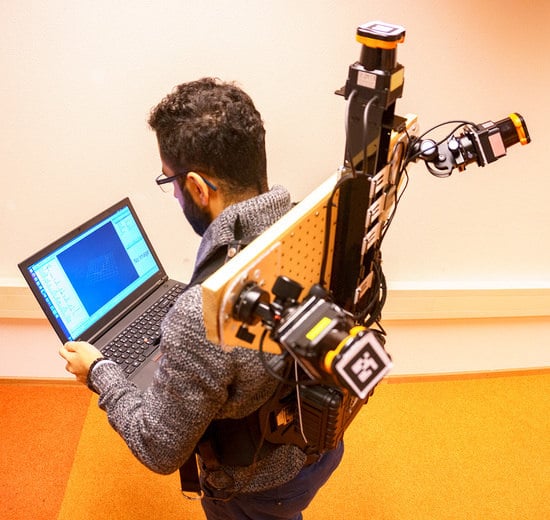
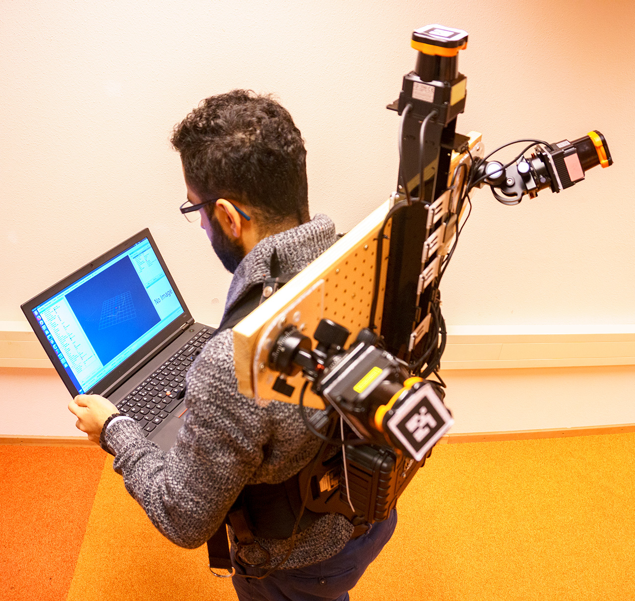
3. Backpack System ITC-IMMS

3.1. System Description

Due to the limited use and problems experienced by the previous indoor mapping systems, we developed our own indoor mobile mapping system shown in Figure 1. Our aim is to combine the proven accuracy of 2D SLAM-based trajectory estimates of push-cart systems with the flexibility of 3D hand-held or backpack systems. The system design has been proposed in [20] and is now implemented, optimised, calibrated, and evaluated. This backpack system consists of three LRFs (Hokuyo UTM-30LX) which are all utilized for a 3D (6 DOF) SLAM. In contrast to available 3D laser scanners, we try to keep the system design less expensive by only making use of these simple LRFs.

The ranging noise according to our LRF’s specifications is ±30 mm for [0.1 10] m range and ±50 mm for [10 30] m range [28]. This gives the Hokuyo UTM-30LX a key advantage over the range camera (Kinect) in capturing data inside large buildings such as airports where the dimensions of interior areas usually exceed 10 m.

The top LRF (here referred to as $S_0$) is mounted on the top of backpack system and it is approximately horizontal while the other two LRFs ($S_1$, $S_2$) are mounted to the right and left of the top one and are rotated around the moving direction (as in the i-MMS) as well as around the operator’s shoulder axis. These two rotation axes are perpendicular to each other as shown in Figure 1. To find the optimal values for the rotation angles, we conducted experiments that will be described in Section 7. There are two objectives for the rotation of the range finders: First, the laser scanning covers surfaces perpendicular to the moving direction e.g., walls both behind and in front of the system, and second, it eases the association of points on new scan lines to previously seen walls. In the case where the scan lines would intersect walls vertically, a strong data association is not guaranteed when walking around corners or through doors. The field of view of the LRFs is limited to 270°, and accordingly, there will be a 90° gap in each scanline. In order to cover all walls as well as possible, the two range finders ($S_1$, $S_2$) are rotated around their axes such that their gaps (shadow areas) are directed towards the floor and the ceiling, respectively [20]. A laptop running Ubuntu 16.04.X and the robot operation system (ROS) is used to communicate with all mounted sensors during data capture.

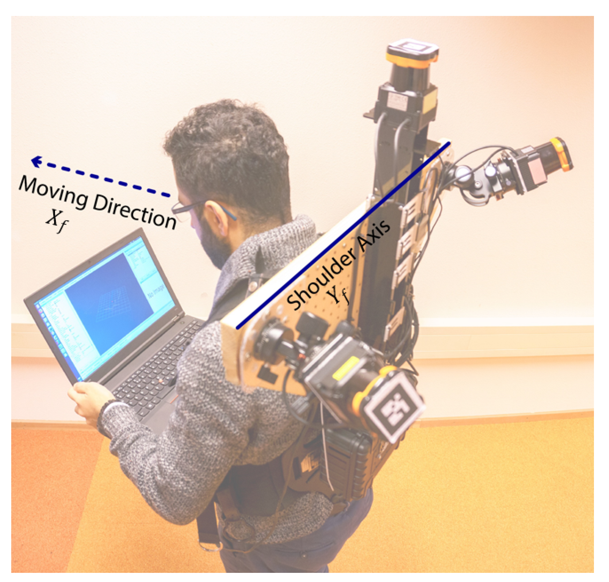
3.2. Coordinate Systems

The proposed mapping system is a multi-sensor system and each one of the three mounted sensors has its own coordinate system. Next to the aforementioned sensor’s coordinate system, there are two additional coordinate systems: the frame (backpack) and model (local world) coordinate system.

To integrate the data of the three LRF sensors, coordinates in their individual coordinate systems must be transformed into a unified coordinate system, which is termed the “frame coordinate system (f)”. We adopt the sensor coordinate system of $S_0$ as the frame coordinate system. Assuming all sensors are rigidly mounted on the frame, the sensor coordinate systems of $S_1$ and $S_2$ are registered in this frame coordinate system using six transformation parameters, namely, three rotation parameters (${\mathsf{\omega }}_{s_i},{\mathsf{\phi }}_{s_i},{\mathsf{\kappa }}_{s_i})$ and three translation parameters $(d{X}_{s_i}, d{Y}_{s_i}, d{Z}_{s_i})$. These parameters are determined in the registration process described in Section 5.

Since the frame coordinate system is attached to a moving backpack system, a fixed coordinate system should be defined as a reference and a space in which the final indoor model will be described. This fixed coordinate system is termed the “model coordinate system (m)”. This model coordinate system is assumed to be the frame coordinate system at the start point of the trajectory. As long as the frame coordinate system is moving in 3D space, it is registered in the model coordinate system using six transformation parameters over time (t), namely, three rotation parameters (${\mathsf{\omega }}_f\left(t\right),{\mathsf{\phi }}_f\left(t\right),{\mathsf{\kappa }}_f\left(t\right))$ and three translation parameters ($d{X}_f\left(t\right), d{Y}_f\left(t\right), d{Z}_f\left(t\right))$. Those changing parameters that originate from the 6DOF SLAM algorithm are explained in more detail in the next section.

3.3. 6DOF SLAM

We defined a feature-based SLAM algorithm in which the range observations of all three scanners contribute to the integral estimation of all six pose parameters. The starting point for the SLAM is the association of newly measured points to already estimated planes in the indoor environment. The six pose parameters are modeled as a function over time using B-splines. The planes are simply defined by a normal vector $\left(n\right)$ and distance to the origin $\left(d\right)$ in the model coordinate system. For a point $X_m$ in the model coordinate system it should therefore hold that:

$$n{X}_m-d=0,$$

(1)

As the laser scanners after registration provide point coordinates $X_f$ in the frame coordinate system, we write $X_m=R\left(t\right) X_f+v\left(t\right)$ to transform a point $X_f$ in the frame coordinate system to point $X_m$ in the model coordinate system by a rotation $R\left(t\right)$ and a translation $v\left(t\right)$. Substituting $X_m$ in Equation (1) provides the observation equation

$$E\left\{n\left[R\left(t\right)X_f+v\left(t\right)\right]-d\right\}=0,$$

(2)

The trajectory of the frame, as well as the rotations, is modelled by B-splines as a function of time $\left(t\right)$. For instance, roll ω is formulated as follow:

$$\omega \left(t\right)={{\displaystyle \sum }}_i{\alpha }_{\omega ,i}.B_i\left(t\right),$$

(3)

where ${\alpha }_{\omega ,i}$ is the spline coefficient for $\omega$ to be estimated on interval $i$.

The model coordinate system is defined based on the first scans of the three scanners. Since there is no information about the system speed yet, the rotation and translation defined during establishing the model coordinate system are used to predict the orientation and translation of the system over the time interval of the first two scanlines using a constant local spline. Later, more data will be captured by the LRFs. Then, for pose parameter prediction, the local spline estimation is implemented using the data of only three to four scanlines of each of the laser scanners. The locally estimated splines are linearly extrapolated to obtain a prediction of the frame pose over the time interval of the next scanline acquisition.

After segmenting the next scanline using a line segmentation procedure [29], a test on a distance threshold is used to decide whether a segment should be associated with an already reconstructed plane or be used to instantiate a new plane need. Currently, only horizontal and vertical planes are used. After setting up the corresponding observation equations, the pose parameters are estimated for the next time interval. After processing the whole dataset with locally defined spline functions, one integral adjustment estimates spline coefficients for the whole trajectory as well as all parameters of planes in the model coordinate system.

4. Calibration Process

In this research the term “calibration” refers to the estimation of biases in the raw range data acquired by every single LRF, in our case the Hokuyo UTM-30LX. The calibration of the laser range finders is needed to optimise the quality of the reconstructed point cloud.

4.1. Calibration Facility

For carrying out the calibration process, a classroom in ITC faculty building was selected as a calibration facility. The room has an almost rectangular shape with white walls and is of a suitable size. The reference data were captured by tape measurements.

4.2. Calibration

Equation (4) formulates the relationship between the coordinates in the LRF sensor system ($X_s, Y_s$), and the model system ($X_m, Y_m$), and Equation (5) describes the known location of a wall in the model system (distance $d$, orientation $\theta$). All relationships are in 2D as we assume the LRF to be scanning perpendicular to the walls.

$$\left(\begin{array}{c}{X}_m\\ Y_m\end{array}\right)=\left(\begin{array}{cc}cos\beta & sin\beta \\ -sin\beta & cos\beta \end{array}\right)\left(\begin{array}{c}{X}_s\\ Y_s\end{array}\right)+\left(\begin{array}{c}{X}_0\\ Y_0\end{array}\right),$$

(4)

$$X_{m}cos\theta +Y_{m}sin\theta -d=0,$$

(5)

where $\beta$ is the rotation of the LRF, and $(X_0, Y_0)$ represent the location of the LRF in the local model coordinate system.

Each indoor environment is decorated differently, and the surface materials are different, e.g., on walls. The surface material properties, e.g., color, brightness, and smoothness, impact the range measurements to a small degree [30]. This change in surface properties to the range measurements is compensated with the calibration of Equation (6). In our calibration model we use a scale factor (${\lambda }_r$) and offset ($\mathsf{\Delta }r$) for the range measurements as well as a scale factor (${\lambda }_{\alpha }$) for the scanning direction. The coordinates in LRF sensor system are obtained from the observed polar coordinates (range $r$, scanning direction $\alpha$).

$$\widehat{r}={\lambda }_{r}r+\mathsf{\Delta }r,$$

(6)

$$\left(\begin{array}{c}{X}_s\\ Y_s\end{array}\right)=\left(\begin{array}{cc}cos{\lambda }_{\alpha }\alpha & sin{\lambda }_{\alpha }\alpha \\ -sin{\lambda }_{\alpha }\alpha & cos{\lambda }_{\alpha }\alpha \end{array}\right)\left(\begin{array}{c}\widehat{r}\\ 0\end{array}\right),$$

(7)

Equations (4)–(7) are combined to obtain a single equation with the pose of the LRF ($X_0$, $Y_0,\beta$) and the calibration parameters (${\lambda }_r$, $\mathsf{\Delta }r$, ${\lambda }_{\alpha }$) as the unknown parameters. The LRF to be calibrated is put on different locations in the calibration room with different rotations to optimise the estimability of the calibration parameters. After a warming up period, the data of a few scan lines per pose are used to estimate all pose and calibration parameters. Points of those scan lines were manually labelled with the index number of the corresponding wall. Estimated range offsets and range scale factors were typically below 4 cm and 0.8%, respectively, whereas the estimated angle scale error is usually below 0.7%. After calibration, the remaining residuals between the points and the wall planes show a root mean square value below 1 cm. This is clearly better than the noise level specified by the manufacturer (3 cm).

4.3. Self-Calibration

Similar to self-calibration in the photogrammetric bundle adjustment, it is feasible to include the estimation of the sensor calibration parameters of all three LRFs in the SLAM process. In absence of a reference (tape) measurement in the SLAM procedure, we can, however, not estimate the range scale factors of all LRFs as the scale of the resulting point cloud would then be undetermined. Hence, we fix the range scale of the top LRF ($S_0$) to the value obtained in the calibration room and include the remaining eight calibration parameters as additional unknowns to the SLAM equations.

5. Relative Sensor Registration

To accurately fuse data from the three LRF sensors, their coordinate systems must be registered to a common reference system. This requires the estimation of the relative pose of the LRFs with respect to each other. We adopt the sensor coordinate system of the horizontal LRF as the backpack frame coordinate system and register as accurately as possible the two slanted LRFs with respect to this system. The registration is performed in two steps: marker registration and fine registration. These processes do not require a room with known dimensions, but the data should be captured in a specific way as described in the following two paragraphs.

5.1. Initial Registration

The registration method is based on 3D tracking technology for markers (see Figure 1) attached to the heads of the mounted LRFs to achieve an approximate registration. We make use of the ‘ar_track_alvar’ package [31], which is a robot operation system (ROS) wrapper for Alvar, an open source library for virtual and augmented reality (AR) marker tracking. As the laptop’s webcam is involved in the registration process, it also needs to be calibrated using another ROS package. As the rotation and translation between the markers and the LRF sensor coordinate systems can be determined to a few mm and degree, the relative marker positions estimated with the ROS package can be used to infer approximate values for the parameters of the relative registration of the three LRFs.

5.2. Fine Registration

The goal of this process is to refine the approximate values for the registration parameters obtained during the previous approach and assumed to be acceptably accurate. This fine registration imposes two constraints on the captured sensor data. As the indoor environment usually contains large planes, the first constraint used is co-planarity of three line segments on the same plane simultaneously scanned by the three LRFs [32,33]. The second constraint is inferred from the perpendicularity of two observed planes [33].

The data collection is carried out with the backpack (ITC-IMMS) on the back of the operator. In order to estimate all registration parameters, the planar surfaces should be observed by the backpack system with different orientations. Therefore, first the operator stands inside a suitable area, in which the previous constraints are applicable, and starts capturing data while bending forward and sideward (right and left). Then, the operator rotates by 90° and bends again in the same way. These rotation and bending steps are repeated until the operator is back at the initial orientation.

The captured data pass through a series of processing steps before being subject to the registration’s constraints. Firstly, the scanlines from each LRF are segmented by a line segmentation algorithm [29] and transformed to a frame system using the approximated parameters. Next, the all pairs of nearly co-planar line segments captured by two different LRFs are collected.

To define the aforementioned constraints, two types of observation equations are formulated, namely, perpendicularity and coplanarity. Let us denote $l_j^i$ as the direction vector of the segment, where i refers to a plane (A, B) and j refers to one of the LRFs (0, 1, 2). The relative transformations of $S_1$ and $S_2$ with respect to $S_0$ are described by 12 parameters, a 3D rotation ($R_1({\omega }_1,{\varphi }_1,{\kappa }_1$) and $R_2({\omega }_2,{\varphi }_2,{\kappa }_2$)) and a 3D translation ($T_1$ and $T_2$) for each.

If two planes A and B are perpendicular it will hold that:

$$\left(l_0^A\times R_1{l}_1^A\right)·\left(l_0^B\times R_1{l}_1^B\right)=0,$$

(8)

where: $l_0^A\times R_1{l}_1^A$ is the normal vector of plane A expressed in the coordinate system of $S_0$, and $l_0^B\times R_1{l}_1^B$ is the normal vector of plane B expressed in the coordinate system of $S_0$. The unknowns in this equation are the rotation angles of $S_1$ in $R_1$.

In a common coordinate system, the two direction vectors of the line segments as well as the vector connecting the midpoints $\left(p_0^i,p_1^i,p_2^i\right)$ must be coplanar. Taking the coordinate system of $S_0$, the coplanarity equation for plane A can be formulated as follows:

$$\left(l_0^A\times R_1{l}_1^A\right)·\left(p_0^A-R_1{p}_1^A-T_1\right)=0,$$

(9)

As three-line segments could be recorded with three different LRFs in each of three perpendicular planes, the data captured at a single pose of the mapping system would yield nine independent coplanarity equations and three independent perpendicularity equations. Thus, this would already provide sufficient observations to estimate all 12 registration parameters. However, to increase the reliability of the estimation we use a much larger number of equations with data of different poses of the backpack captured according to the described bending procedure. The scanning frequency of the Hokuyo used is 40 Hz; therefore, after one minute, each LRF records 2400 scanlines thereby leading to a very large number of observation equations.

Using the available approximated values from marker registration and after linearizing the formulated equations, an accurate estimate of the transformation parameters can be obtained by applying a least-squares estimation. The standard deviations of the estimated parameters are around 1 mm for the translations and around 0.05° for the rotation angles.

5.3. Self-Registration

In analogy to the self-calibration for the intrinsic sensor parameters of the LRFs, we can also extend the SLAM equations with the parameters describing the relative poses of the LRFs. We refer to this registration approach as the self-registration. Approximate values of the 12 registration parameters are obtained from either the initial registration or fine registration described above. When the sensor data are captured with a good variation in the rotations of the backpack with respect to the surrounding walls, ceiling and floor, as realized by the bending procedure, all 12 self-registration parameters can be estimated well as part of the overall estimation of all pose spline coefficients and plane parameters. This is not the case when the backpack IMLS is used in a normal mode when the operator walks upright through a building. In that case the top LRF, scanning in an approximately horizontal plane, will only capture vertical walls. As a consequence, the vertical offset between this LRF and the other two cannot be estimated. In this scenario the self-registration is restricted to 11 parameters.

6. SLAM Performance Measurements and Results

This section elaborates the methodology to evaluate indoor laser scanning point clouds described in our previous work [5] with some additions. Moreover, the measurements taken by our mapping system (ITC-IMMS) are processed by applying this methodology to investigate the performance of the 6DOF SLAM and to assess the capability of ITC-IMMS of capturing the true geometry of building interiors and preserve an accurate positioning when moving from one room to another.

6.1. Dataset

The dataset used is collected by ITC-IMMS at the University of Braunschweig, Germany. The scanned area shows a distinct office environment that has many windows and doors leading to rooms. Due to renovation work, the rooms were nearly empty. On the one side, this allows an easier identification of planar surfaces. On the other side, the number of surfaces is relatively small and a missed surface may have a larger impact on the estimability of the pose spline coefficients. The generated point cloud and the reconstructed planes are shown in Figure 2. About 73 million points were captured during a 9-minute walk through the rooms.

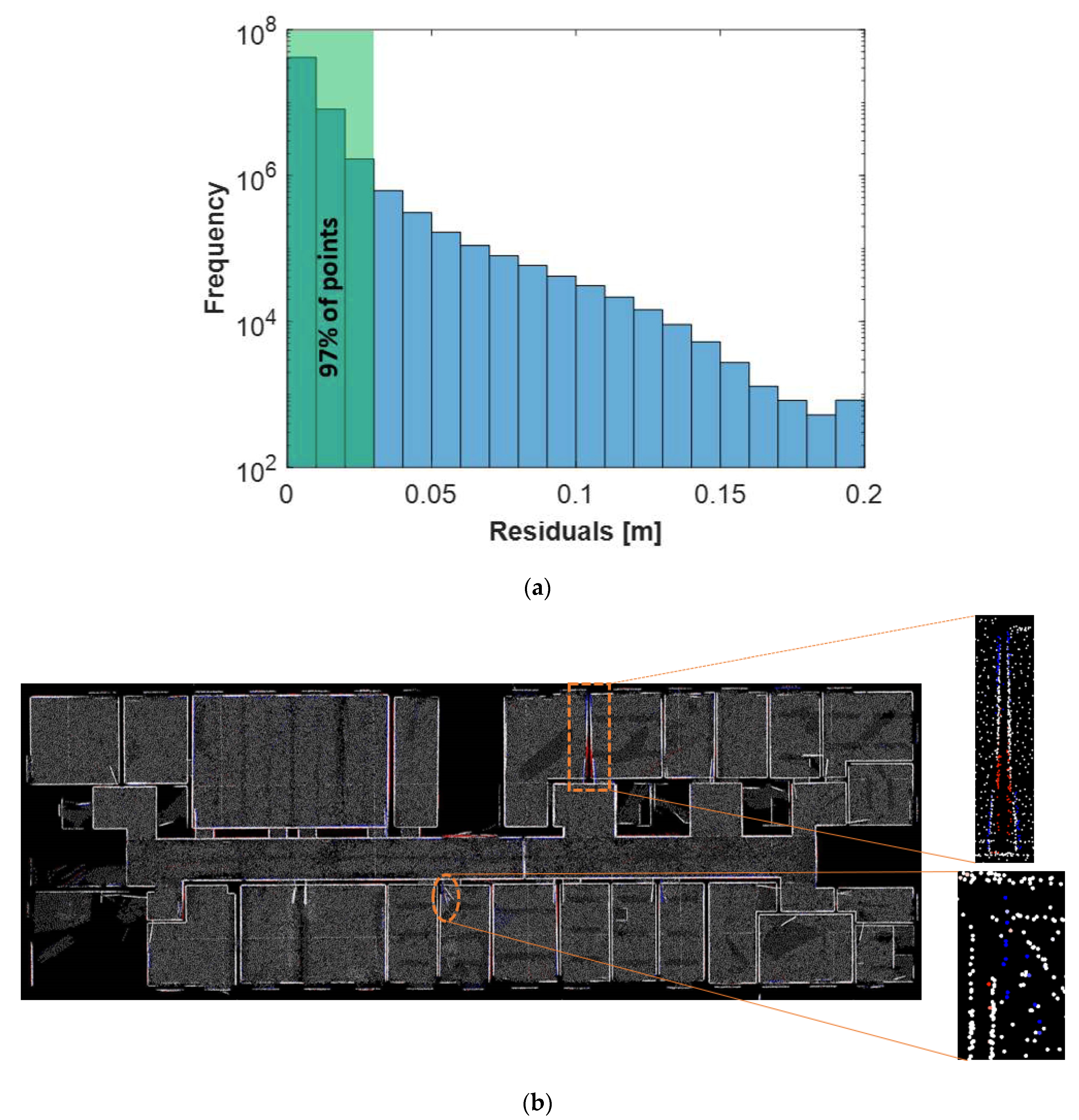
Point to Plane Association (Data Association)

The point is assigned to the closest plane if its distance to this plane is lower than 20 cm. Of the 73 million points, 53 million points were associated to 503 planes during the SLAM and used to estimate a total of 27880 pose spline coefficients and plane parameters. The distribution of the residual distance from the point to its associated plane is shown in Figure 3a. In total, 97% of the points have residuals below 3 cm and the RMS value of these residuals is only 1.3 cm. This means that the method is self-consistent. The RMS value, however, does not adequately represent the overall quality of the dataset. Further quality measures are therefore developed and used in the next section.

Figure 3b shows a top view of the generated point cloud, where points are colored based on their respective residuals. The data association rule which assigns points to planes experiences problems when two distinct planes are too close to each other. For example, a door that is wide open and thus close to the wall, or a door that is only slightly open and thus close to the other wall are typical causes for this behaviour. Moreover, there can be dynamic noise, for instance, if a door is opening while the data is being captured. Clear examples of both problematic cases are highlighted in Figure 3b. The problem resulting from merging a door with a nearby wall can be seen inside the orange dashed rectangle.

6.2. Evaluation Techniques

As SLAM-based point clouds usually suffer from registration errors because of the dead-reckoning nature of SLAM algorithms, the performance of the mapping system and the accuracy of the provided results, which needs to be analyzed. While most current evaluation methods rely on the availability of reference data, we develop several techniques to investigate the mapping system in the absence of an accurate ground truth model. The proposed techniques take advantage of regularities in wall configurations to check how well the rooms are connected, and thus how well the environment is reconstructed.

Since most buildings have a floor plan (though often outdated), we utilize that as an external information source to check the quality of the generated indoor model, but without relying on an accurate registration of the point cloud to the floor plan. We classify the developed techniques into three independent groups: (1) techniques using architectural constraints; (2) techniques using a floor plan; and (3) completeness techniques.

To simplify the process and because the permanent structure of man-made indoor environments mainly consists of planar and vertical structures, the first two groups make use of 2D edges derived from such structures. As our feature-based SLAM outputs both point clouds and 3D reconstructed planes, the 2D edges are derived from the projection of the vertical planes onto the XY-plane, as presented in our previous work [5]. We address the third group of evaluation techniques in the study of the optimal configuration described in Section 7.

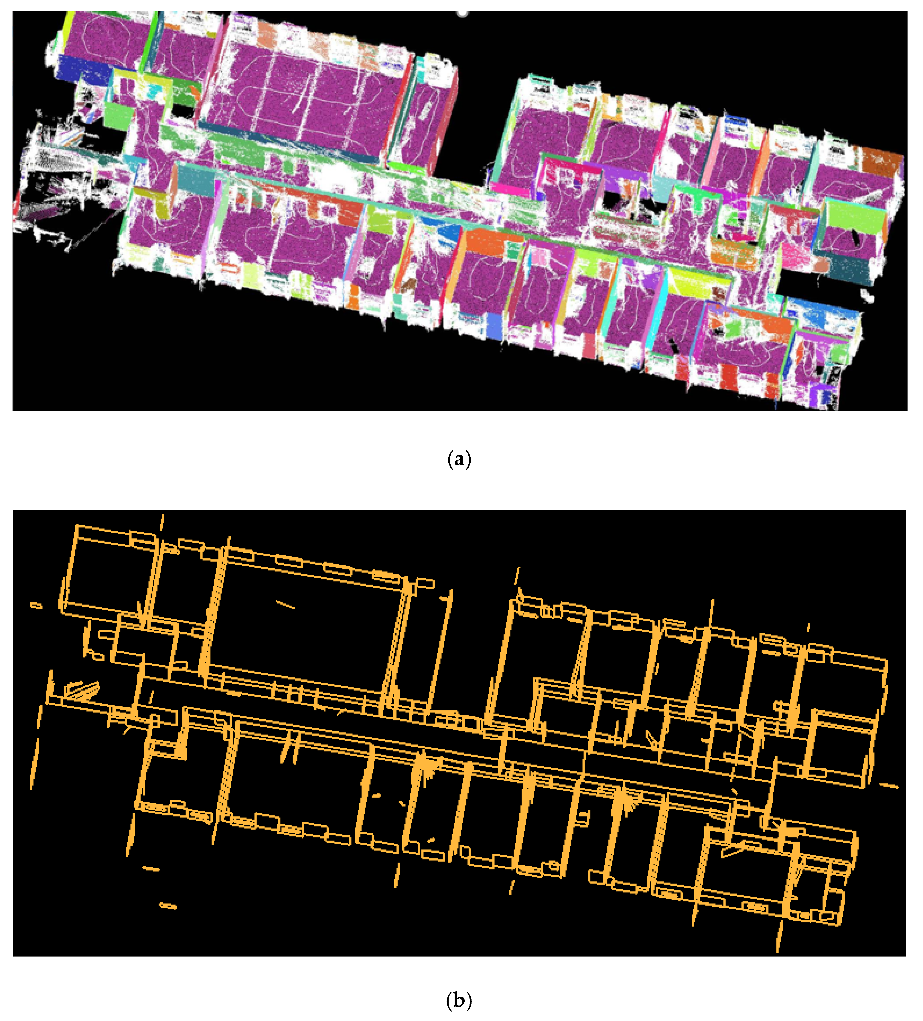
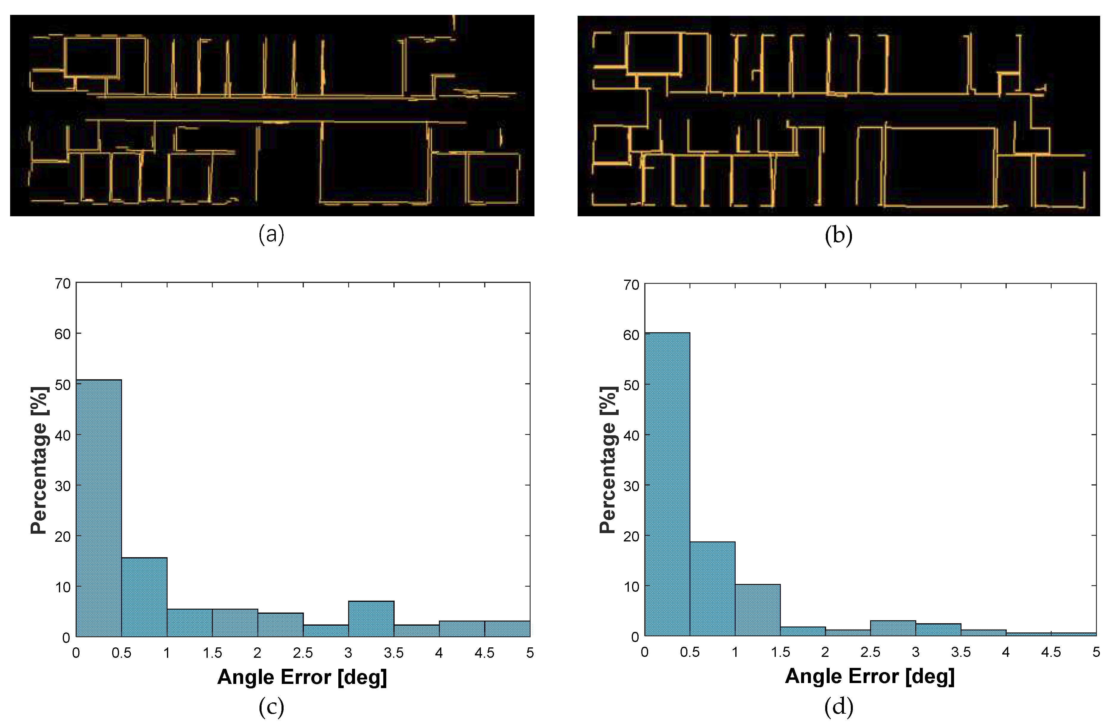
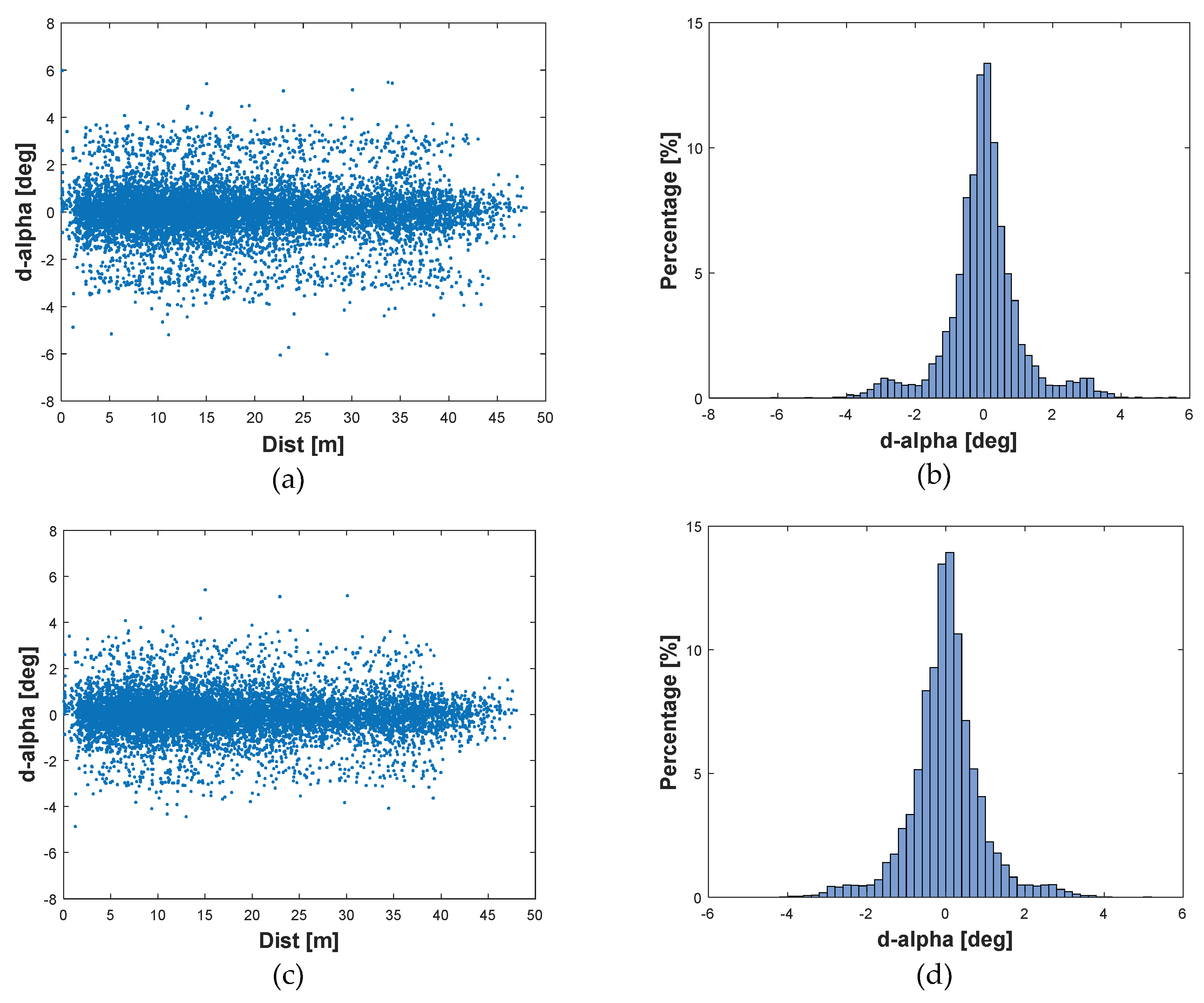
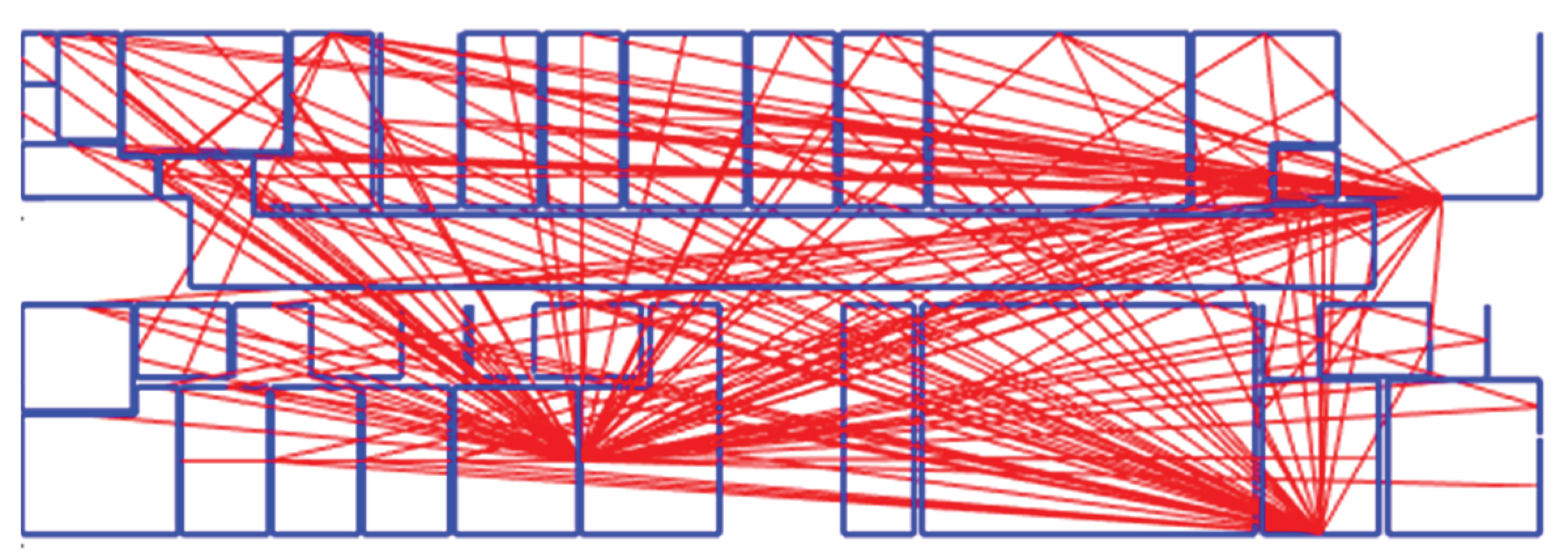
6.2.1. Evaluation Using Architectural Constraints

We make use of the predominant characteristics in indoor man-made environments, namely, perpendicularity and parallelism of walls, to investigate the ability of our mapping system to capture the true geometry of the mapped environment. Two sides of a particular wall are parallel and two neighbouring walls in a room are usually perpendicular. Thus, the corresponding reconstructed pairs of planes resulting from the indoor mapping should be both parallel or perpendicular as well. Nearly perpendicular pairs of planes with nearby endpoints are labelled as perpendicular edges. Nearly parallel planes at a short distance and with opposite normal vector directions are labelled as parallel edges. Moreover, we make a histogram of the estimated wall thickness. As most walls will have the same thickness in reality, we expect a clear peak in this histogram. The angles between the planes at opposite wall sides and the wall thickness histogram provide a good impression of the ability of the mapping system to maintain an accurate positioning when moving from one room to another.

We assume two walls to be perpendicular when the angle between their 2D edges in the XY plane is between 85° and 95° and their end points, that are close to the intersection point and should represent the corner point, are within 30 cm. Furthermore, the angle between the parallel edges should be below 5° and the distance between them should not exceed 30 cm. The results of the Braunschweig data are shown in Figure 4a,b. In addition, we compute the angle error as the deviation from the perfect parallelism (0°) and perpendicularity (90°) and build histograms of these errors as shown in Figure 4c,d. In reality walls are, of course, never constructed perfectly parallel or perpendicular to other walls, but the deviation from this is expected to be an order of magnitude smaller than the deviations observed in the reconstructed model.

The results show that the angle between two sides of a wall is determined less accurately than that between two perpendicular planes in the same room. This is consistent with the expected performance of SLAM algorithms, as the two walls sides are not seen at the same point of time. Moreover, we note high percentages in the above histograms in bins where the angles deviate by more than 2.5° from their expected values of 0° and 90°. By tracking the source of these high percentages, we found that they mainly originate from incorrectly reconstructed planes, such as open doors. In addition, the measurements of walls’ thickness demonstrate that there are two standard types of walls in the building and the standard deviation of the thickness is around 1 cm.

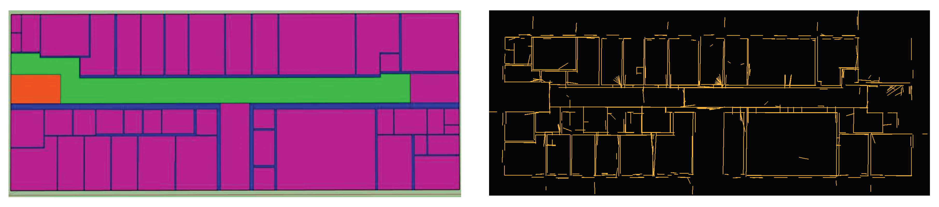
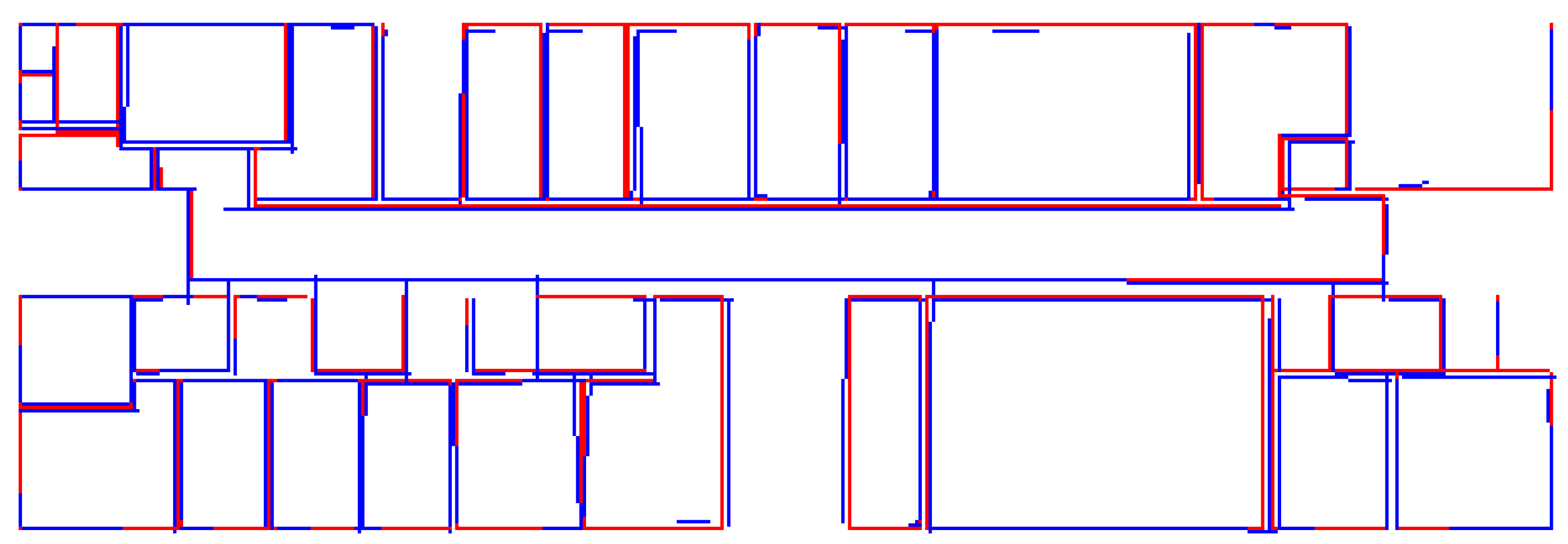
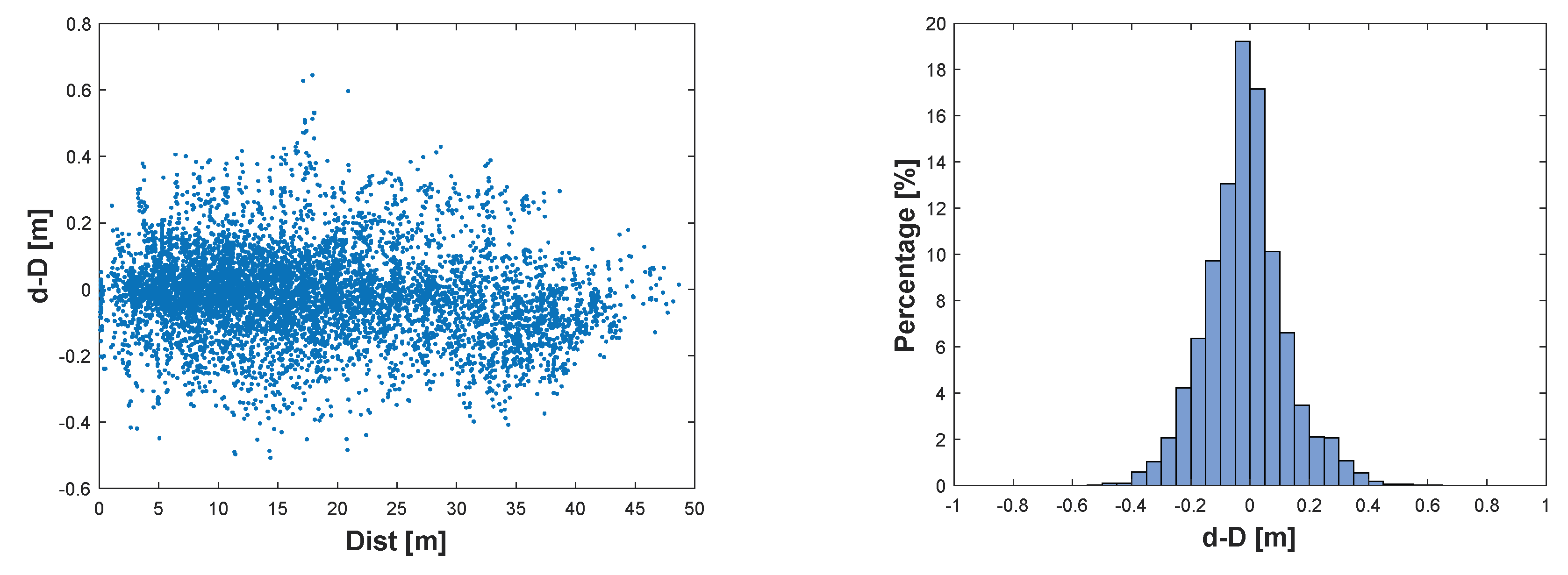
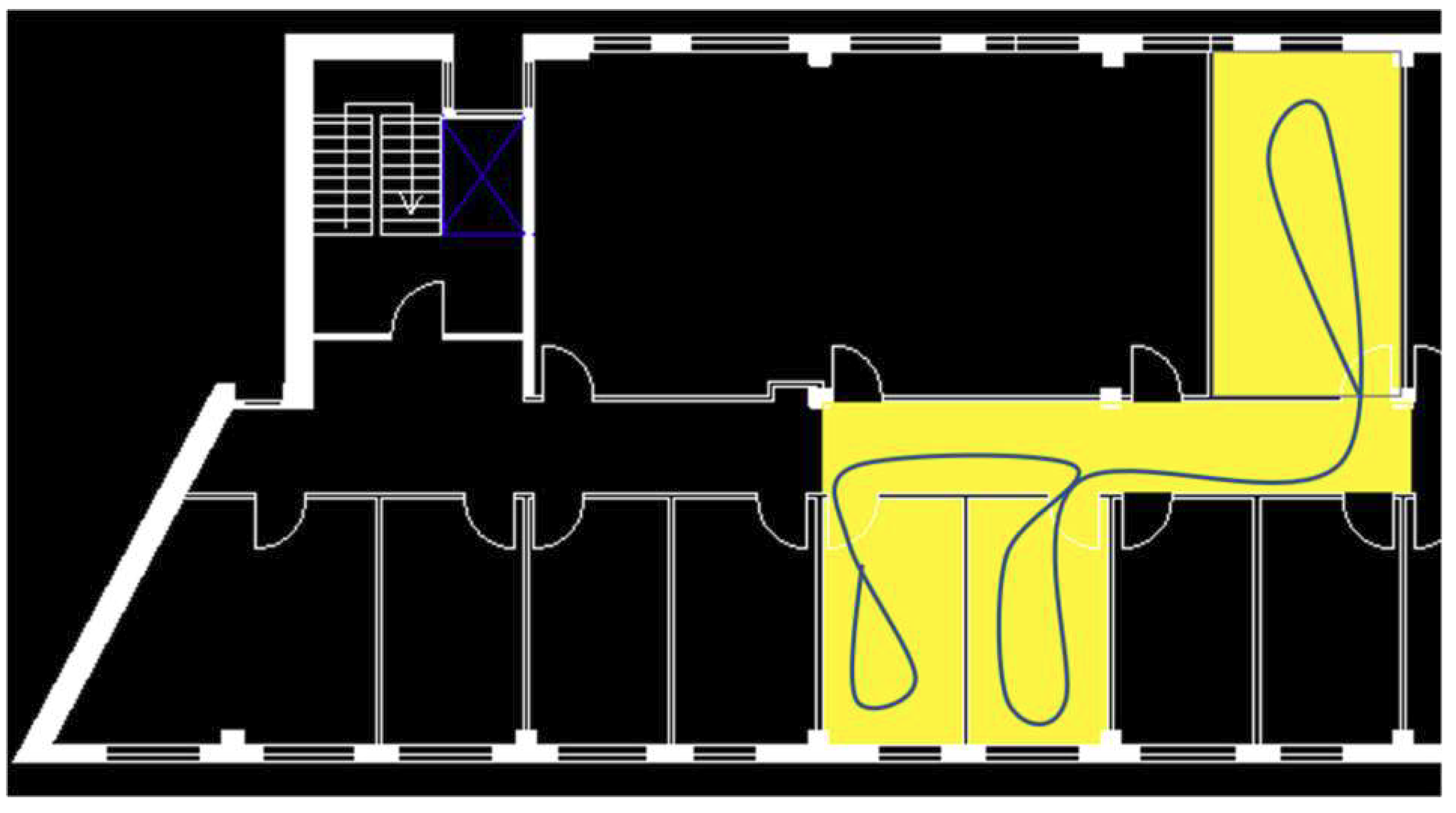
6.2.2. Evaluation Using a Floor Plan

Nowadays, many buildings have 2D floor plans reflecting the as-planned state from before construction. We investigate the feasibility of using a simple 2D floor plan in analyzing the accuracy of the reconstructed model.

Transformation: As the 2D edges derived from our SLAM-based point clouds and those in the floor plan (see Figure 5) are in two different coordinate systems, we have to register them in the same coordinate system for valid comparison. We use a 2D similarity transformation and estimate the transformation parameters based on a number of manually selected corresponding points. The main goal of this transformation is to identify correspondences between the edges extracted from the point cloud and those in the floor plan. We do not estimate residual distances or angles between an edge in the point cloud and an edge in the floor plan, because we want to keep the comparison process independent of the chosen coordinate systems and quality of the registration. Therefore, we only compare the angles and distances between edges or points extracted from the point cloud to the angles and distances between the corresponding edges or points in the floor plan. The left image in Figure 5 shows the digitized floor plan of the scanned floor.

Edge Matching: When both sets of edges are registered in the same coordinate system, we start matching the corresponding edges. Firstly, we detect all point cloud-based edges that are expected to belong to a room in the floor plan using a buffer around the room polygon, termed a polygon-buffer. Secondly, we choose which of the detected edges most probably represents the side of a wall in that room using another buffer (30 cm width) around each of the room’s edges, termed an edge-buffer as well as the normal vector direction to avoid confusion with edges of the opposite wall side.

In contrast to other objects, walls usually are reconstructed as large and more reliable planes in the SLAM process. Therefore, a further selection based on height information is implemented to keep only edges that most probably belong to walls. We implement the filtering process room by room in order to estimate the floor and ceiling height for each room separately and exclude non-wall edges based on their height. An edge is classified as a window-edge and removed if the corresponding plane is not connected to either the floor or ceiling, and if its height is less than 2 m. Similarly, an edge is classified as a door-edge and removed if the corresponding plane is connected to the floor and its height is less than 2.2 m. Thus, the remaining edges ${\mathit{E}}_{\mathit{P}\mathit{C}}$, that most probably represent walls in the building, form what we term the PC-based map. Figure 6 shows the resulting PC-based map consists of 144 edges matched to the floor plan edges ${\mathit{E}}_{\mathit{F}}$.

Analysis: The final step is to pair edges from both edge sets (${\mathit{E}}_{\mathit{P}\mathit{C}} , {\mathit{E}}_{\mathit{F}}$) and form a set of tuples of matched edges. Based on these set of edges, we perform the statistical computations needed to check the accuracy of the PC-based map, and thus the accuracy of generated point clouds.

a) Error in angle in relation to distance

We want to study the impact of distance on the angle errors. Let ${\mathit{E}}_{\mathit{P}\mathit{C}}$ and ${\mathit{E}}_{\mathit{F}}$ be edge sets extracted from the point cloud and floor plan, respectively. Let ${(e_{pc}, e_F)}_i$ be pairs of matched edges where $i=1,2, \dots , n$ and $n$ is the number of pairs. We pick the $i^{th}$ pair of edges ${(e_{pc}, e_F)}_i$ and compute the angles ${({\alpha }_{pc}, {\alpha }_F)}_{ij}$ and distances ${(d_{mf})}_{ij}$ with respect to all other pairs of edges ${(e_{pc}, e_F)}_j$ where ${\left({\alpha }_F\right)}_{ij}$ is the angle between ${(e_F)}_i$ and ${(e_F)}_j$, ${\left({\alpha }_{pc}\right)}_{ij}$ is the angle between ${(e_{pc})}_i$ and ${(e_{pc})}_j$, ${(d_{mf})}_{ij}$ is the distance between midpoints of ${(e_F)}_i$ and ${(e_F)}_j$, and $j=i+1, i+2, \dots , n$. For each pair of edges, we compute the difference between the angle in the point cloud and angle in the floor plan: ${(\mathsf{\Delta }\alpha ={\alpha }_{pc}- {\alpha }_F)}_{ij}$. Hence, we obtain $n\left(n-1\right)/2$ angle differences and the corresponding distances between the edges $\left(\mathsf{\Delta }\alpha , d_{mf}\right)$. We compute these values for the Braunschweig data where 10296 pairs of edges are examined to obtain the results displayed in Figure 7.

The results presented in Figure 7a,b demonstrate that the errors in the angle between point cloud edges are small; approximately 81% are in the range [−1°, 1°]. The two remarkable small peaks in Figure 7b around ±3° refer to some larger errors which may belong to only a few poorly reconstructed planes. Overall, as can be seen in Figure 7a, the distance between edges has no impact on the error in the angle between them.

To identify the poorly estimated outlier edges, we construct Figure 8 in which all edges pairs that have an angle error of 3° or more are presented. The pattern in this figure clearly indicates which edges are mostly involved in edge pairs with large angle errors. We observed five outlier edges and excluded them from the computations in order to obtain a better picture of the potential quality of the system; see Figure 7c,d.

Table 1. Values of mean, standard deviation, and the number of edges pairs that are involved in the computations for both cases, before and after excluding outlier edges.

	Before	After
Mean	0.01°	0.00°
Std Dev.	1.14°	0.85°
Edge-Pairs Nr	10296	9591

shows standard deviation values and the number of edge pairs that are involved in the computations for both cases, both before and after excluding outlier edges. We can see that the removal of the outlier edges leads to a 25% decrease in the estimated standard deviation.

Since the perpendicular and parallel edges are already labelled (Section 3.2), we also computed these values for each type of edge separately. We found that the error in the angle over distance is not related to the attitude of one edge to other. Moreover, we studied the impact of time on the angle errors as the 3D planes are reconstructed over time through applying the SLAM algorithm. However, the results show no relation between time and angle errors. The reason for this is that the operator returned to the same corridor during the data capturing in Braunschweig which in turn leads to frequent loop closures that prevent the errors from accumulating.

b) Error in distance in relation to distance:

Besides the previous computations of angle errors based on the pairs of edges, we compute the distance errors based on pairs of edges’ end points. However, because the point cloud-based map is usually incomplete, we find corner points by intersecting the neighbouring edges. We utilize the topology of the floor plan and intersect edges from ${\mathit{E}}_{\mathit{P}\mathit{C}}$ if their matched floor plan edges $e_F$ are connected.

Let $P_{pc}$ and $P_F$ be intersection points obtained from the floor plan and the point cloud, respectively. Let ${(p_{pc}, p_F)}_i$ be pairs of points where $i=1,2, \dots , n$ and $n$ is the number of pairs. We pick the $i^{th}$ pair of points ${(p_{pc}, p_F)}_i$ and compute the distances ${(d_{pc}, d_f)}_{ij}$ with respect to all other pairs of points ${(p_{pc}, p_F)}_j$ where ${(d_f)}_{ij}$ is the distance between ${(p_F)}_i$ and ${(p_F)}_j$, ${(d_{pc})}_{ij}$ is the distance between ${(p_{pc})}_i$ and ${(p_{pc})}_j$, and j $=i+1, i+2, \dots , n$. Next, the error in the distances ${(\mathsf{\Delta }d=d_f-d_{pc})}_{ij}$ will be plotted against the distances ${(d_f)}_{ij}$ to check if the error in distance depends on the distance between floor plan points. Computing the error in distance in this way will remove the systematic error that would otherwise result from errors in the transformation.

From the data used, we obtain 128 corner points leading to 8128 pairs of points involved in the distance errors computation as function of distance. Figure 9 shows that the errors in distance are sometimes quite large (~40 cm). The source of such error is not necessarily the mapping system or the proposed SLAM algorithm, but it could be also the outdated floor plan used. We noted some differences in the width of some walls between the floor plan and the realised construction.

We carried out an analysis similar to that shown in Figure 8 to identify the poorly reconstructed corners (outlier points) using the distance between $p_{pc}$ and $p_F$. The comparison of the results before and after excluding these outlier points does not show a significant improvement. However, it is not possible to draw the conclusion that these errors are caused by the ground truth model used or the mapping system.

7. Determining Optimal Configuration

As our system is equipped with several sensors, we utilize the proposed evaluation techniques in the previous section to find the optimal configuration.

7.1. Studied Configurations

It is important to avoid occlusion and to acquire sufficient geometrical information of the building to be mapped. As our mapping system is composed of three 2D sensors, we seek the optimal mount of these sensors (LRFs) on the backpack by making use of the proposed evaluation methods above. The optimal sensor configuration is defined through an experimental comparison of different configurations.

The experiments were conducted in an indoor office environment at our university. The three selected rooms, with a corridor in-between, were captured by the system for several possible configurations. A set of criteria was used to select the studied configurations.

In order to see all walls around the system, $S_0$ is always be horizontal and above the operator’s head, and only rotatable around its rotational axis. As the Hokuyo LRF has a 270° field of view, we rotate $S_0$ around its axis in such a way that the shadow area (gap) points to the left or right side of the operator in order to achieve a good coverage of the surfaces both behind and in front of the system.

In contrast to the top LRF, the left and right LRFs ($S_1$, $S_2$) have three rotational degrees of freedom around three axes: the operator’s moving direction ($X_f)$, the operator’s shoulder axis $\left(Y_f\right),$ and the LRF’s rotational axis (see Figure 1). However, some points need to be considered in these rotations. For a good data association, it is better to mount $S_1$ and $S_2$ in a way that they scan in two different planes. The oblique scanlines provide a good coverage of walls behind and in front of the system and ensure the overlap with old data when passing through doors and corners. Also, this geometry of the scanlines provides sufficient observations that strengthen the system of equations and make the pose estimation process more robust [21].

Nevertheless, we found empirically that a small angle of rotation around the shoulder axis leads to a better coverage of the surfaces around the system, while a wide angle of rotation may lead to a loss of coverage of the floor and ceiling. Thus, this reduces the estimability of the system’s movement in z direction. To avoid occlusion by the operator’s body, we should have forward-slanted scanlines.

Based on the aforementioned criteria, a set of orientation configurations for the two LRFs as listed in

Table 2. Tested configurations are defined by the first five columns (explained in Section 7.1) and the results from the three distinct evaluation techniques are listed in the last five columns (explained in Section 7.2). The resulting values are highlighted with colors, as follows. For RMSE: < 0.80° green, [0.80°, 1°] yellow, and ≥ 1° red. For λ expressed in percentages: [85, 100] green, [70, 85] yellow, and ≤ 70 red. The last column represents the completeness state of the point cloud in three different cases: existence of large gaps, existence of small gaps, or almost no gaps.

Orientation Configuration of LRFs	${\mathit{\theta }}_1 \left[\mathbf{deg}\right]$		${\mathit{\theta }}_2 \left[\mathbf{deg}\right]$		Arch. Constraints		loor Plan		Gap
	${\mathit{S}}_1$	${\mathit{S}}_2$	${\mathit{S}}_1$	${\mathit{S}}_2$	RMSE [deg]	λ %	RMSE [deg]	λ %	Size
1	20 1	20 1	20 2	20 2	1.57	70	0.79	67	Small
2	30	30	30	30	0.81	85	0.40	85	No
3	40	40	40	40	0.94	83	0.56	76	No
4	15	20	30	30	0.94	84	0.57	73	Small
5	30	30	20	20	0.76	90	0.51	79	No
6	20	20	40	40	0.54	95	0.71	83	Small
7	40	40	20	20	0.77	86	0.57	74	No
8	20	20	30	30	1.38	83	0.82	72	Small
9	0	20	20	90	1.25	81	0.76	70	Large
10	0	30	30	90	0.65	99	0.54	87	Large
11	0	40	40	90	0.73	91	0.52	80	Large

¹ The LRF is rotated 20° around the moving direction and 20° is the angle between its scanline plane and the horizontal plane ${(XY)}_f$. ² The LRF is rotated 70° (i.e., 90° − 20°) around the shoulder axis, but 20° is the angle between its scanline plane and the vertical plane ${(YZ)}_f$.

was tested. Specifically, the table lists the rotations of LRFs $S_1$ and $S_2$, namely, ${\theta }_1$ and ${\theta }_2$, around the moving direction ($X_f$) and the shoulder axis ($Y_f$), respectively. In addition, the LRFs are rotated around their axis to ensure that the gap of one points to the floor and the gap of other points to the ceiling. This provides as many observations as possible on all surfaces (walls, floor, and ceiling) in order to position the backpack.

7.2. Experimental Comparison of Configurations

For each suggested configuration, we find the relative orientation of the slanted LRFs ($S_1$, $S_2$) with respect to the horizontal LRF $\left(S_0\right)$ with the registration procedures explained in Section 5. Next, we scan the test area with all possible configurations and each time, we obtain a dataset of point cloud and 3D reconstructed planes.

7.2.1. Accuracy

Evaluation Using Architectural Constraints: The test area consists of rectangular rooms as can be seen in Figure 10. Regarding the analysis of the perpendicularity, the basic approach explained in Section 6.2.1 is extended to involve all walls that should be perpendicular to each other in the building and not only the neighboring walls in a room. Similarly, the algorithm looks for all walls that should be parallel to each other in the building and not only both sides of a wall. Next, we compute the Root Mean Square Error (RMSE) of the computed angles to estimate the deviations from the perfect perpendicularity and parallelism, respectively.

Evaluation Using the Floor Plan: The floor plan of the test area is available as a 2D CAD drawing; see Figure 10. The evaluation of errors in angles and distances is conducted as described in Section 6.2.2 for the Braunschweig dataset.

All the resulting statistical values for both architectural constraints and using the floor plan are listed in Table 2. The comparison between the listed configurations is done using these values which reflect the reconstruction accuracy. The sixth column presents the sum of RMSE values computed in the two evaluation techniques introduced before (perpendicularity, parallelism) for each configuration (see Section 6.2.1). Also, for each configuration, we count the points that have an angle error of less than 1° and divide this amount by the total number of points, yielding a rate of angle errors λ. We take the average rate in these two techniques (perpendicularity, parallelism) and present the results in the seventh column. Similarly, the eighth and ninth columns in Table 2 demonstrate the computed RMSE and λ computed for each configuration with the availability of floor plan. These statistical values are computed in order to get an overall impression of the reconstruction accuracy of each configuration, and thus it helps in decision making on the optimal configuration.

The sixth and seventh columns in the Table 2 show that the configurations (1, 8, 9) have clearly larger deviations than the other configurations, therefore being less accurate in capturing the geometry of the building interiors. The evaluation using the floor plan, as shown in the eighth and ninth columns, confirms this conclusion. RMSE values for parallelism indicate that the configurations (2–7, 10, 11) are the most accurate in maintaining an accurate localization when moving from one room to another. The common characteristic of these configurations is that they have at least one of the two rotation angles in the range of 30° to 40°.

7.2.2. Completeness of Data Capturing

We visually inspect the completeness of the captured data in which walls, floor, and ceiling are recorded. The process relies on a simulated point cloud representing a scan of a virtual corridor (loop) and generated for each configuration. Figure 11a shows the 3D model of this virtual area and Figure 11b the point cloud of configuration 6 where the colors relate to the three different LRFs and the white polyline represents the followed trajectory. The simulated point cloud generating process assumes the operator walks around the corridor in an anti-clockwise direction starting from the middle of the corridor.

The analysis process is based on a set of point clouds corresponding to all suggested configurations to compare the areas covered by points and find which configuration provides the better coverage. We want to investigate whether a more accurate configuration in geometry reconstruction provides a more complete point cloud of the scene.

Overall, configurations (1–8) appear to give a good coverage. However, the configurations (2, 3, 5, 7) provide the most complete point cloud of the scene, while the LRFs with the other configurations miss the lower/upper part of the wall in the scanning geometry when the system turns around the corner. An example of a configuration (6) that results in an incomplete point cloud is shown in Figure 11b. This configuration misses a part of the wall close to the corner (see Figure 11c). Figure 11d shows the data recorded in one scan line of each LRF in the configuration 6. The tenth column in Table 2 demonstrates that the configurations (9, 10, 11) have the largest gaps in their point clouds. The common characteristic of these configurations is that only one of the slanted LRFs is scanning the walls both right and left of the system.

7.3. Discussion of Configuration Experiments

The results of Section 7.1 and Section 7.2 lead to the conclusion that the more accurate configuration in geometry reconstruction does not necessarily provides a more complete point cloud of the scene, and vice versa. Although the configurations (10, 11) show a better performance than configurations (2, 8) in terms of the reconstruction accuracy, they provide a less complete point cloud.

Finally, our system has the top LRF mounted horizontally and on a level that the environment is not occluded by the operator’s head. The shadow area of this LRF is pointed to the walls to the left or right of the operator. We discovered that the other two LRFs should be scanning the surfaces parallel to the moving direction e.g., walls both right and left of the system. Also, we found out that these LRFs should be rotated not only about the shoulder axis ($Y_f$), but at least one of them should also be rotated around the moving direction ($X_f$) by an angle in the range of 30° to 40°. Moreover, the results revealed that determining where the LRFs’ data gap is pointing at plays a pivotal role in the completeness of the resulting point clouds. The best coverage is achieved when the gap of one slanted LRF is aimed at the floor and the gap of other is aimed at the ceiling.

8. Conclusions

We presented the design, calibration and registration methods, and performance analysis of a multi-sensor backpack indoor mobile mapping system (ITC-IMMS). We have proposed and presented several evaluation techniques for the investigation of the system’s ability to acquire geometric information of an interior environment. Evaluations can also be performed when there is no ground truth model or only a floor plan available. If the floor plan is outdated, this will usually surface as a large error in the evaluation and can therefore be identified as outlier. The results on the Braunschweig data showed some differences in the width of some walls between the floor plan and the realized construction. Such changed walls can then be removed from the map. The proposed evaluation methods are not limited to our mapping system.

The experimental results showed the ability of ITC-IMMS to map an office building with an angle error within 1.5° between its planar surfaces, and the precision in generating the width of wall is around 1 cm. Although we did not consider the errors in the outdated floor plan, the point cloud-based map shows a good internal consistency.

We have carried out an experimental comparison of selected configurations to find the best configuration by studying the properties of 3D planes and point clouds reconstructed with these configurations. The selection of the optimal sensor configuration was built in terms of data occlusion, the success of the algorithm, and the accuracy and completeness of the resulting map and point cloud. In order to see all walls around the system, we left the top LRF mounted horizontally in the optimal configuration for the backpack system and on a level that the environment cannot be occluded by the operator’s head. To achieve a good coverage of the surfaces both behind and in front of the system, it must be rotated around its axis to locate the shadow area on the walls to the left or right of the operator. The other two LRFs should be scanning in a plane perpendicular to the moving direction. Also, they should be rotated not only about the shoulder axis, but at least one of them should also be rotated about the moving direction by an angle in the range of 30° to 40°. The gap of one should be pointed at the floor, while the gap of other should be pointed at the ceiling. In this way, the system achieves improved coverage of the environment and ensures a good data association when passing through doors and corners, and thus has a robust estimation of the plane and pose parameters.

Nevertheless, the analysis of the system’s performance may be slightly different in another indoor environment with much larger or smaller spaces. For such environments we would then need to repeat the experiments of Section 7, but we do not expect this will be necessary for many buildings.

In the near future, we plan to expand the scope of application of the current system and SLAM algorithm to include more complex situations such as staircases and fancy architecture (e.g., slanted walls, round walls, non-horizontal floor). To do that, we will integrate IMU data in the local pose estimation and as consequence, we can use higher order splines to predict future poses. We anticipate that this integration will lead to a better hypothesis generation of planar structures and an optimal estimation for the whole trajectory.

References

1. Biber, P.; Andreasson, H.; Duckett, T.; Schilling, A. 3D modeling of indoor environments by a mobile robot with a laser scanner and panoramic camera. In Proceedings of the 2004 IEEE/RSJ International Conference on Intelligent Robots and Systems (IROS), Las Vegas, NV, USA, 28 September–2 October 2004; Volume 4, pp. 3430–3435. [Google Scholar]
2. Borrmann, D.; Elseberg, J.; Lingemann, K.; Nüchter, A.; Hertzberg, J. Globally consistent 3D mapping with scan matching. Rob. Auton. Syst. 2008, 56, 130–142. [Google Scholar] [CrossRef] [Green Version]
3. Henry, P.; Krainin, M.; Herbst, E.; Ren, X.; Fox, D. RGB-D Mapping: Using Depth Cameras for Dense 3D Modeling of Indoor Environments. In Experimental Robotics, Springer Tracts in Advanced Robotics; Springer: Berlin/Heidelberg, Germany, 2014; Volume 79, pp. 477–491. [Google Scholar]
4. Lehtola, V.V.; Kaartinen, H.; Nüchter, A.; Kaijaluoto, R.; Kukko, A.; Litkey, P.; Honkavaara, E.; Rosnell, T.; Vaaja, M.T.; Virtanen, J.P.; et al. Comparison of the selected state-of-the-art 3D indoor scanning and point cloud generation methods. Remote Sens. 2017, 9, 796. [Google Scholar] [CrossRef]
5. Karam, S.; Peter, M.; Hosseinyalamdary, S.; Vosselman, G. An Evaluation Pipeline for Indoor Laser Scanning Point Clouds. ISPRS Ann. Photogramm. Remote Sens. Spat. Inf. Sci. 2018, 4, 85–92. [Google Scholar] [CrossRef]
6. Bosse, M.; Zlot, R.; Flick, P. Zebedee: Design of a spring-mounted 3-D range sensor with application to mobile mapping. IEEE Trans. Robot. 2012, 28, 1104–1119. [Google Scholar] [CrossRef]
7. Viametris iMS3D-VIAMETRIS. Available online: http://www.viametris.com/products/ims3d/ (accessed on 20 November 2018).
8. Trimble Applanix: TIMMS Indoor Mapping. Available online: https://www.applanix.com/products/timms-indoor-mapping.htm (accessed on 20 November 2018).
9. Wen, C.; Pan, S.; Wang, C.; Li, J. An Indoor Backpack System for 2-D and 3-D Mapping of Building Interiors. IEEE Geosci. Remote Sens. Lett. 2016, 13, 992–996. [Google Scholar] [CrossRef]
10. Blaser, S.; Cavegn, S.; Nebiker, S. Development of a portable high performance mobile mapping system using the robot operation system. ISPRS Ann. Photogramm. Remote Sens. Spat. Inf. Sci. 2018, 4, 13–20. [Google Scholar] [CrossRef]
11. Naikal, N.; Kua, J.; Chen, G.; Zakhor, A. Image Augmented Laser Scan Matching for Indoor Dead Reckoning. In Proceedings of the 2009 IEEE/RSJ International Conference on Intelligent Robots and Systems, St. Louis, MO, USA, 10–15 October 2009; pp. 4134–4141. [Google Scholar]
12. Lehtola, V.V.; Virtanen, J.-P.; Vaaja, M.T.; Hyyppä, H.; Nüchter, A. Localization of a mobile laser scanner via dimensional reduction. ISPRS J. Photogramm. Remote Sens. 2016, 121, 48–59. [Google Scholar] [CrossRef]
13. Leica Geosystems. Leica Pegasus: Backpack. Available online: https://leica-geosystems.com/ (accessed on 4 February 2019).
14. Chen, G.; Kua, J.; Shum, S.; Naikal, N.; Carlberg, M.; Zakhor, A. Indoor localization algorithms for a human-operated backpack system. In Proceedings 3D Data Processing, Visualization, and Transmission; University of California: Berkeley, CA, USA, 2010; pp. 15–17. [Google Scholar]
15. Liu, T.; Carlberg, M.; Chen, G.; Chen, J.; Kua, J.; Zakhor, A. Indoor localization and visualization using a human-operated backpack system. In Proceedings of the 2010 International Conference on Indoor Positioning and Indoor Navigation, Zurich, Switzerland, 15–17 September 2010; pp. 1–10. [Google Scholar]
16. Thomson, C.; Apostolopoulos, G.; Backes, D.; Boehm, J. Mobile Laser Scanning for Indoor Modelling. ISPRS Ann. Photogramm. Remote Sens. Spat. Inf. Sci. 2013, 2, 289–293. [Google Scholar] [CrossRef]
17. Maboudi, M.; Bánhidi, D.; Gerke, M. Evaluation of Indoor Mobile Mapping Systems. In Proceedings of the GFaI Workshop 3D North East 2017, Berlin, Germany, 7–8 December 2017; pp. 125–134. [Google Scholar]
18. Maboudi, M.; Bánhidi, D.; Gerke, M. Investigation of geometric performance of an indoor mobile mapping system. ISPRS Arch. Photogramm. Remote Sens. Spat. Inf. Sci. 2018, 42, 637–642. [Google Scholar] [CrossRef]
19. Tran, H.; Khoshelham, K.; Kealy, A. Geometric comparison and quality evaluation of 3D models of indoor environments. ISPRS J. Photogramm. Remote Sens. 2019, 149, 29–39. [Google Scholar] [CrossRef]
20. Vosselman, G. Design of an indoor mapping system using three 2D laser scanners and 6 DOF SLAM. ISPRS Ann. Photogramm. Remote Sens. Spat. Inf. Sci. 2014, 2, 173–179. [Google Scholar] [CrossRef]
21. GeoSLAM GeoSLAM—The Experts in ‘Go-Anywhere’ 3D Mobile Mapping Technology. Available online: https://geoslam.com/ (accessed on 25 November 2018).
22. VIAMETRIS iMS2D-VIAMETRIS. Available online: http://www.viametris.com/products/ims2d/ (accessed on 4 December 2018).
23. Kim, B.K. Indoor localization and point cloud generation for building interior modeling. In Proceedings of the IEEE RO-MAN, Gyeongju, Korea, 26–29 August 2013; pp. 186–191. [Google Scholar]
24. Filgueira, A.; Arias, P.; Bueno, M. Novel inspection system, backpack-based, for 3D modelling of indoor scenes. In Proceedings of the 2016 International Conference on Indoor Positioning and Indoor Navigation (IPIN), Alcalá Henares, Spain, 4–7 October 2016; pp. 4–7. [Google Scholar]
25. Zhang, J.; Singh, S. LOAM: Lidar Odometry and Mapping in Real-Time. In Proceedings of the Robotics: Science and Systems Foundation, Berkeley, CA, USA, 12–16 July 2014. [Google Scholar] [CrossRef]
26. Lagüela, S.; Dorado, I.; Gesto, M.; Arias, P.; Gonz, D.; Lorenzo, H. Behavior analysis of novel wearable indoor mapping system based on 3D-SLAM. Sensors 2018, 18, 766. [Google Scholar] [CrossRef] [PubMed]
27. Sirmacek, B.; Shen, Y.; Lindenbergh, R.; Zlatanova, S.; Diakite, A. Comparison of ZEB1 and Leica C10 indoor laser scanning point clouds. ISPRS Ann. Photogramm. Remote Sens. Spat. Inf. Sci. 2016, 143–149. [Google Scholar] [CrossRef]
28. Hokuyo Ltd. Hokuyo Automatic Co., Ltd. Available online: https://www.hokuyo-aut.jp/ (accessed on 4 December 2018).
29. Peter, M.; Jafri, S.R.U.N.; Vosselman, G. Line segmentation of 2D laser scanner point clouds for indoor SLAM based on a range of residuals. ISPRS Ann. Photogramm. Remote Sens. Spat. Inf. Sci. 2017, 4, 363–369. [Google Scholar] [CrossRef]
30. Park, C.-S.; Kim, D.; You, B.-J.; Oh, S.-R. Characterization of the Hokuyo UBG-04LX-F01 2D laser rangefinder. In Proceedings of the 19th International Symposium in Robot and Human Interactive Communication, Viareggio, Italy, 13–15 September 2010; pp. 385–390. [Google Scholar]
31. Niekum, S. ar_track_alvar-ROS Wiki. 2013. Available online: http://wiki.ros.org/ar_track_alvar (accessed on 25 November 2018).
32. Fernández-Moral, E.; Arévalo, V.; González-Jiménez, J. Extrinsic calibration of a set of 2D laser rangefinders. In Proceedings of the 2015 IEEE International Conference on Robotics and Automation (ICRA), Seattle, WA, USA, 26–30 May 2015; pp. 2098–2104. [Google Scholar] [CrossRef]
33. Choi, D.G.; Bok, Y.; Kim, J.S.; Kweon, I.S. Extrinsic calibration of 2D laser sensors. In Proceedings of the 2014 IEEE International Conference on Robotics and Automation (ICRA), Hong Kong, China, 31 May–7 June 2014; pp. 3027–3033. [Google Scholar] [CrossRef]
Figure 1. The laptop used and the backpack system mounted by three LRFs S 0 (Top), S 1 (left), and S 2 (right) fitted with markers.
Remotesensing 11 00905 g001
Figure 2. ITC-IMMS outputs. (a) The generated point cloud (colors show plane association) with the trajectory followed (white). (b) The reconstructed planes.
Remotesensing 11 00905 g002
Figure 3. The residuals between the points and the estimated planes. (a) Frequency of the residuals with a logarithmic scale for the y-axis and a linear scale for the x-axis. (b) Top view of the generated point cloud. All white points have residuals below 3 cm and points with larger residuals are marked with either red or blue color, depending on the sign. The orange dashed rectangle marks an example of a plane representing a door being merged with another plane, which represents a wall that is near the door. The orange dashed oval surrounds an opening door.
Remotesensing 11 00905 g003
Figure 4. The results of the architectural constraints method. (a) All pairs of parallel edges. (b) All pairs of perpendicular edges. (c) Percentages of angle errors between parallel edges in the range [0°, 5°]. (d) Percentages of angle errors between perpendicular edges in the range [85°, 95°].
Remotesensing 11 00905 g004
Figure 5. The digitized floor plan (left) and point cloud-based edges for Braunschweig data (right).
Remotesensing 11 00905 g005
Figure 6. The final point cloud edges E P C (blue) that match the floor plan edges E F (red).
Remotesensing 11 00905 g006
Figure 7. (a) Errors in angle as relation of distance. (b) Histogram of the percentages of errors. (c) Errors in angle as a function of distance after excluding outlier edges. (d) Histogram of the percentages of errors after excluding outlier edges.
Remotesensing 11 00905 g007
Figure 8. Red lines for edge pairs (blue) that have an angle error of 3° or more.
Remotesensing 11 00905 g008
Figure 9. Errors in distance in relation to the distance (left) and Histogram of the percentages of errors (right).
Remotesensing 11 00905 g009
Figure 10. Part of the 2D CAD drawing of the 3rd floor in the Citadel building with highlighted scanning area (yellow) and the trajectory followed (blue).
Remotesensing 11 00905 g010
Figure 11. Simulation data. (a) 3D model of the virtual corridor used as a test area with the trajectory followed (white). (b) The resulting point cloud of the test area for the configuration 6 without ceiling’s points. The yellow dashed rectangle shows an example of a gap on the wall around the corner (c). (d) The simulated geometry of LRFs’ scanlines for the configuration 6 in which the colors relate to the three different LRFs ( S 0   g r e e n ,   S 1   p u r p l e ,   S 2 red).
Remotesensing 11 00905 g011