A Precise and Robust Segmentation-Based Lidar Localization System for Automated Urban Driving


Abstract
:
1. Introduction
- A novel efficient low-level semantic segmentation-based feature extraction algorithm is designed to extract multiple types of stable features from the online frames, including ground, road-curb, edge, and surface. They ensure accurate pose estimation for frame-frame and frame-map matching.
- A priori information considered category matching method and a multi-group-step L-M [11] (Levenberg Marquardt) optimization algorithm are proposed, which can avoid most of the mismatching to improve the accuracy, and increase the efficiency by reducing the Jacobian matrix dimension.
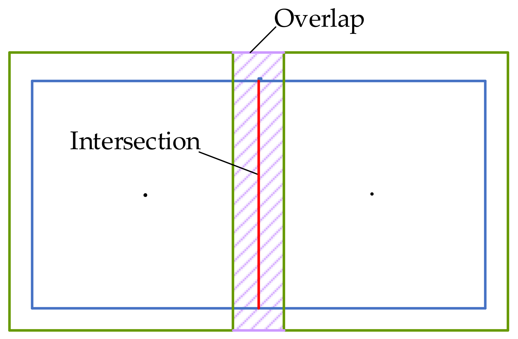
- An efficient priori map management is presented, the map is stored in tiles with overlap and the local map surrounding the vehicle is dynamically loaded to save the computation resource.
- A complex and complete vehicle localization system has been accomplished by integrating all modules reasonably, which can provide high-accuracy and real-time localization service for high-level unmanned vehicles in various challenging scenes and harsh weather.
2. Related Works
3. Methodology
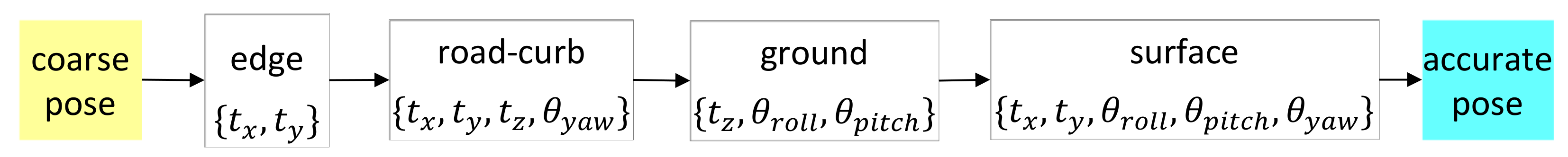
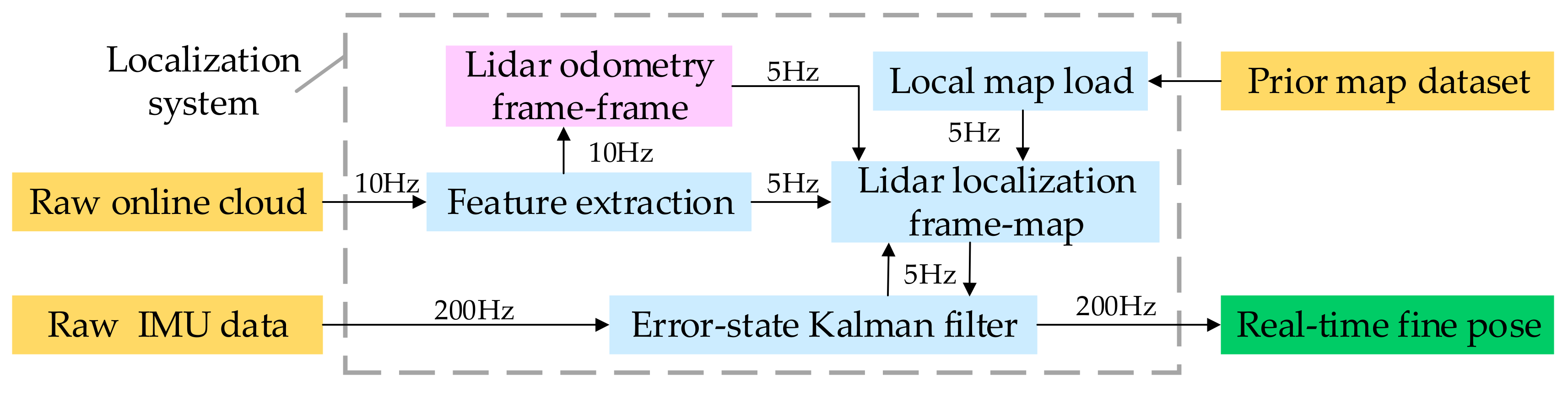
3.1. System Overview
| Algorithm 1. Lidar Localization System |
| Input: prior map , online point cloud at 10 Hz, IMU data at 200 Hz. |
| Output: fine pose . |
| 1: establish the error-state Kalman filter , and pushback the IMU data into ; |
| 2: for frame do |
| 3: delete the dynamic object within the road; |
| 4: based on low-level semantic segmentation, extract the feature point cloud road , road_curb , surface , and edge from the remaining point cloud in turn; |
| 5: if initialized then |
| 6: calculate the transform between the and from IMU odometry queue; |
| 7: else |
| 8: get by category matching with ; |
| 9: end if |
| 10: calculate the rough pose ; |
| 11: dynamically update and load the local map ; |
| 12: category match with , and use as the initial value to get the fine pose by multi-group-step L-M optimization; |
| 13: pushback into ; |
| 14: end for |
| 15: calculate the final fine pose using , and output at 200 Hz; |
| 16: return ; |
3.2. Lidar Feature Map Management
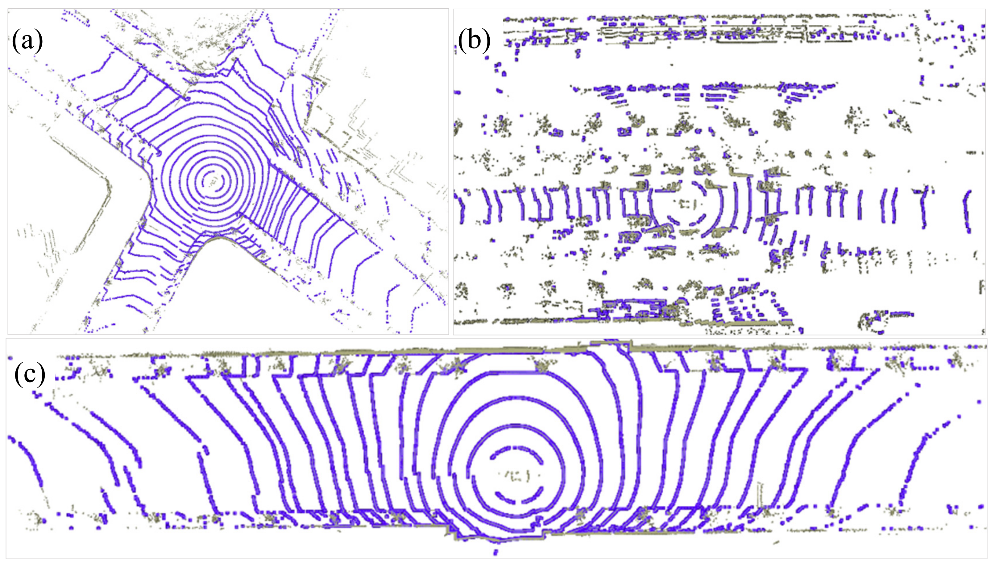
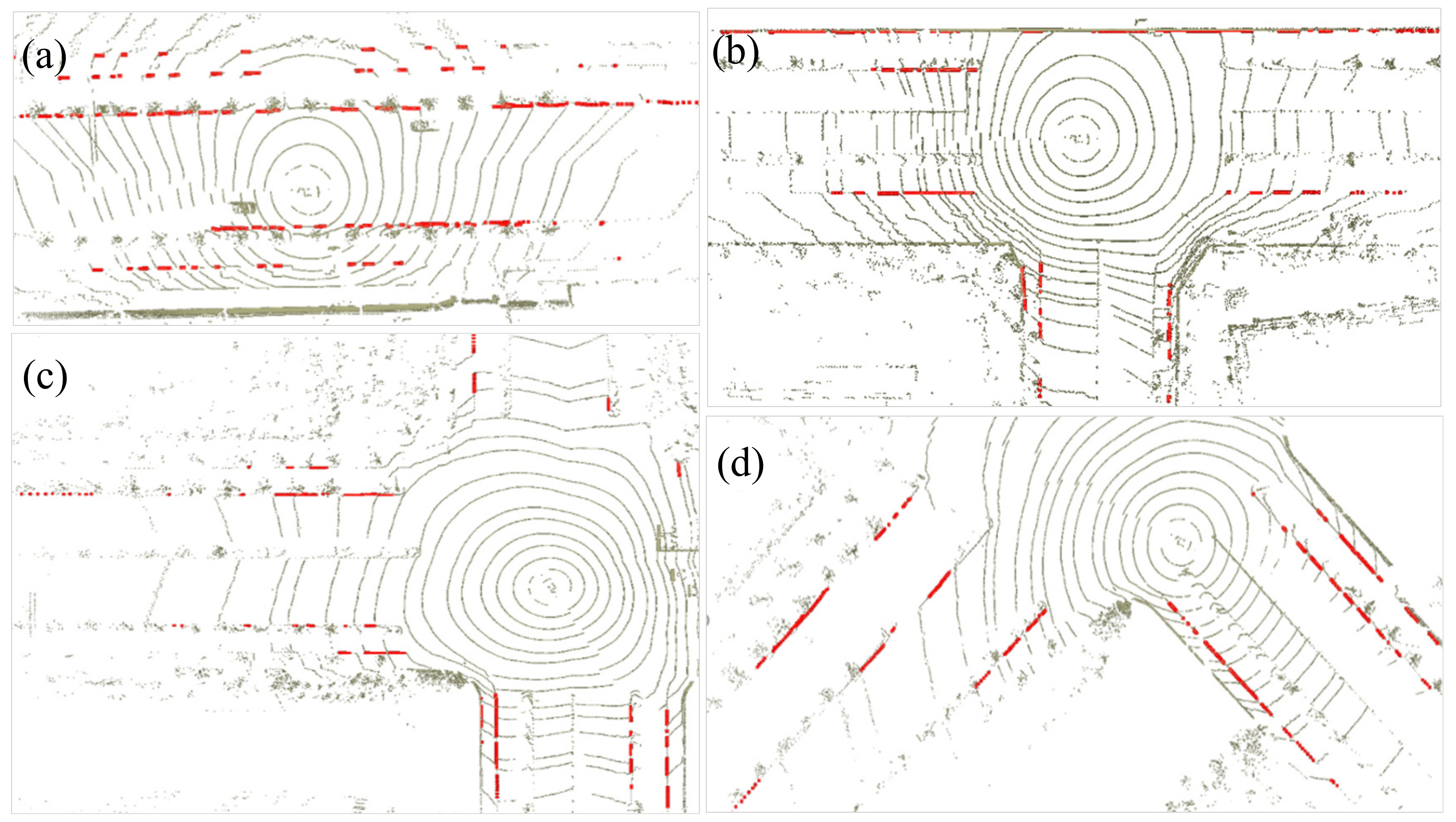
3.3. Segmentation-Based Feature Extraction
3.3.1. Ground
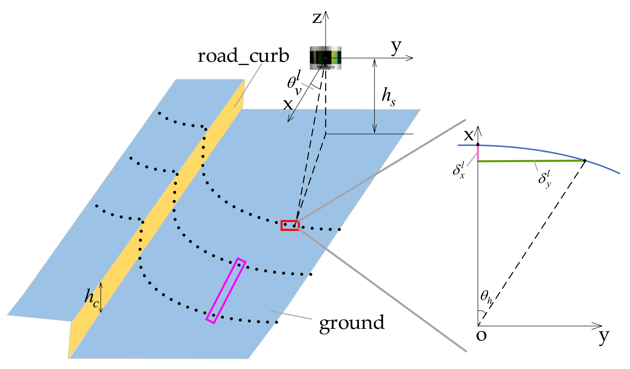
3.3.2. Road-Curb
3.3.3. Surface
3.3.4. Edge
3.4. Priori Information Considered Category Matching
3.5. Multi-Group-Step L-M Optimization
3.6. Lidar and IMU Fusion
4. Experiment Results and Discussions
4.1. Hardware System and Evaluation Method
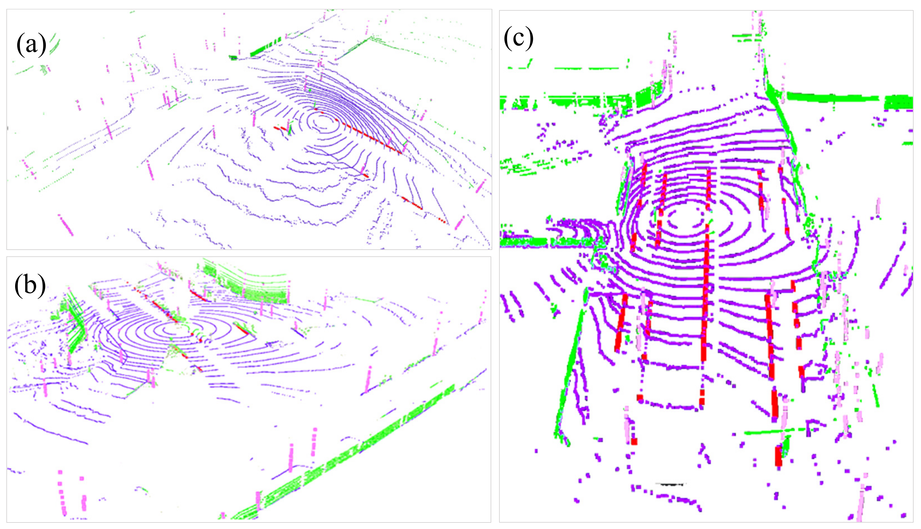
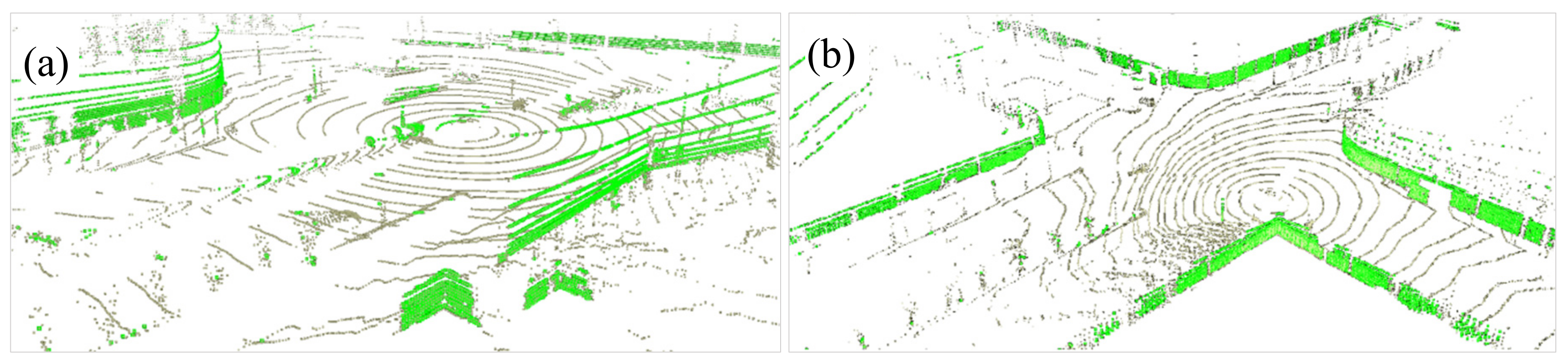
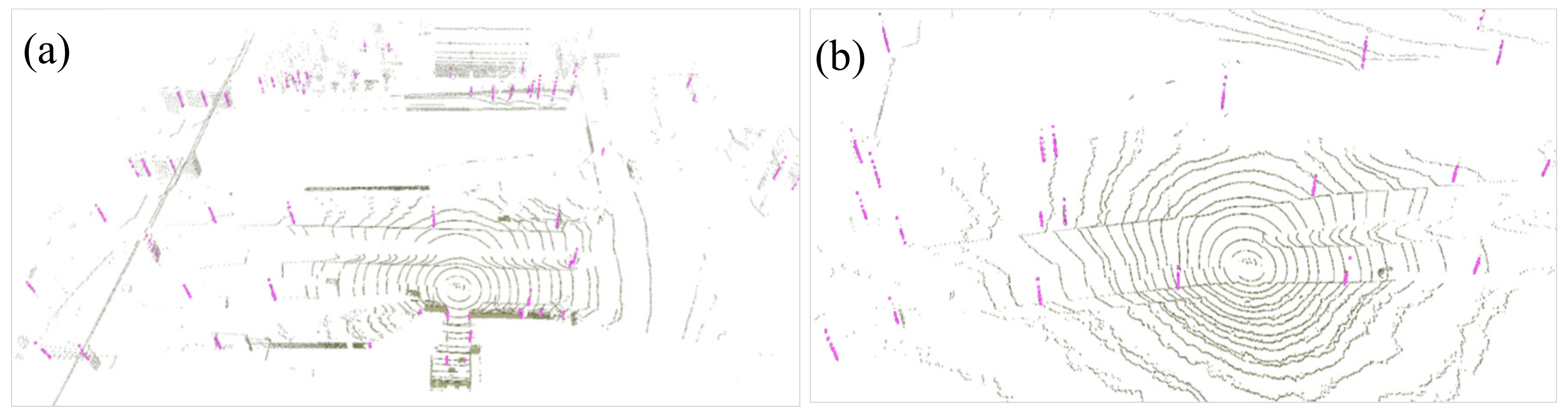
4.2. Segmentation-Based Feature Extraction Result Analysis
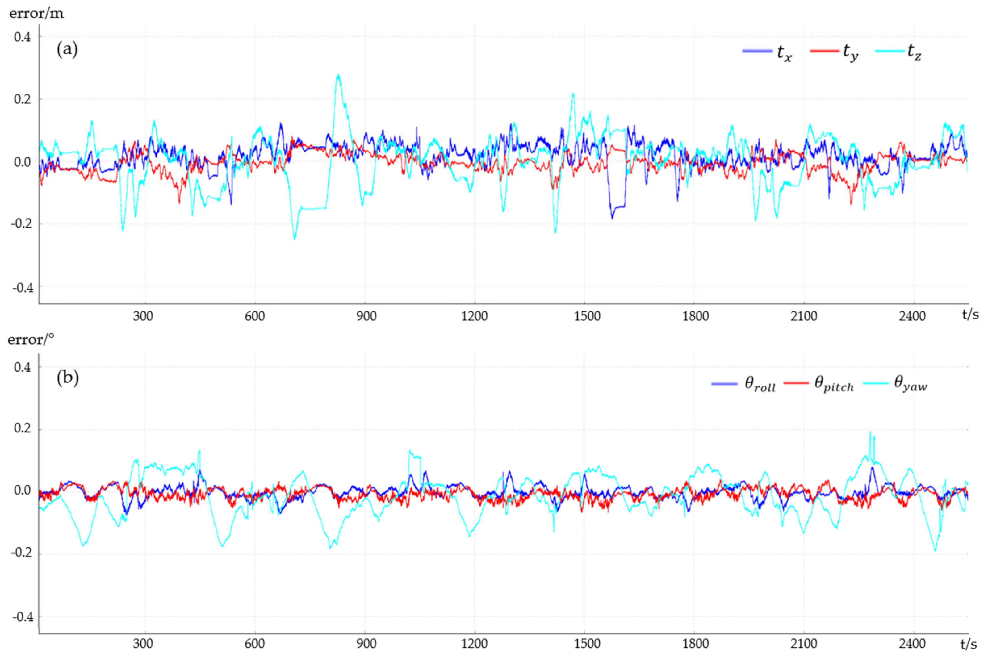
4.3. Qualitative and Quantitative Analysis of Localization Accuracy
5. Conclusions
Author Contributions
Funding
Acknowledgments
Conflicts of Interest
References
- Groves, P.D. Principles of GNSS, Inertial, and Multisensor Integrated Navigation Systems; Artech House: Fitchburg, MA, USA, 2013. [Google Scholar]
- Falco, G.; Pini, M.; Marucco, G. Loose and tight GNSS/INS integrations: Comparison of performance assessed in real urban scenarios. Sensors 2017, 17, 255. [Google Scholar] [CrossRef] [PubMed]
- Zhang, X.; Miao, L.; Shao, H. Tracking architecture based on dual-filter with state feedback and its application in ultra-tight GPS/INS integration. Sensors 2016, 16, 627. [Google Scholar] [CrossRef]
- Wei, W.; Zongyu, L.; Rongrong, X. INS/GPS/Pseudolite integrated navigation for land vehicle in urban canyon environments. In Proceedings of the IEEE Conference on Cybernetics and Intelligent Systems, Singapore, 1–3 December 2004; pp. 1183–1186. [Google Scholar]
- Woo, R.; Yang, E.J.; Seo, D.W. A Fuzzy-Innovation-Based Adaptive Kalman Filter for Enhanced Vehicle Positioning in Dense Urban Environments. Sensors 2019, 19, 1142. [Google Scholar] [CrossRef] [PubMed]
- Choi, K.; Suhr, J.; Jung, H. FAST Pre-Filtering-Based Real Time Road Sign Detection for Low-Cost Vehicle Localization. Sensors 2018, 18, 3590. [Google Scholar] [CrossRef] [PubMed]
- Wang, D.; Xu, X.; Zhu, Y. A Novel Hybrid of a Fading Filter and an Extreme Learning Machine for GPS/INS during GPS Outages. Sensors 2018, 18, 3863. [Google Scholar] [CrossRef] [PubMed]
- Van Brummelen, J.; O’Brien, M.; Gruyer, D.; Najjaran, H. Autonomous vehicle perception: The technology of today and tomorrow. Transp. Res. Part C Emerg. Technol. 2018, 89, 384–406. [Google Scholar] [CrossRef]
- Castorena, J.; Agarwal, S. Ground-edge-based LIDAR localization without a reflectivity calibration for autonomous driving. IEEE Robot. Autom. Lett. 2018, 3, 344–351. [Google Scholar] [CrossRef]
- Gawel, A.; Cieslewski, T.; Dubé, R.; Bosse, M.; Siegwart, R.; Nieto, J. Structure-based vision-laser matching. In Proceedings of the IEEE/RSJ International Conference on Intelligent Robots and Systems (IROS), Daejeon, Korea, 9–14 October 2016; pp. 182–188. [Google Scholar]
- Roweis, S. Levenberg-Marquardt Optimization; University Of Toronto: Toronto, ON, Canada, 1996. [Google Scholar]
- Hsu, C.M.; Shiu, C.W. 3D LiDAR-Based Precision Vehicle Localization with Movable Region Constraints. Sensors 2019, 19, 942. [Google Scholar] [CrossRef] [PubMed]
- Forster, C.; Pizzoli, M.; Scaramuzza, D. SVO: Fast semi-direct monocular visual odometry. In Proceedings of the IEEE international conference on robotics and automation (ICRA), Hong Kong, China, 31 May–7 June 2014; pp. 15–22. [Google Scholar]
- Engel, J.; Schöps, T.; Cremers, D. LSD-SLAM: Large-scale direct monocular SLAM. In Proceedings of the European Conference on Computer Vision (ECCV), Zurich, Switzerland, 6–12 September 2014; pp. 834–849. [Google Scholar]
- Qin, T.; Li, P.; Shen, S. Relocalization, global optimization and map merging for monocular visual-inertial SLAM. In Proceedings of the IEEE International Conference on Robotics and Automation (ICRA), Brisbane, Australia, 21–26 May 2018; pp. 1197–1204. [Google Scholar]
- Weiss, S.; Achtelik, M.W.; Lynen, S.; Chli, M.; Siegwart, R. Real-time onboard visual-inertial state estimation and self-calibration of mavs in unknown environments. In Proceedings of the IEEE International Conference on Robotics and Automation, St. Paul, MN, USA, 14–18 May 2012; pp. 957–964. [Google Scholar]
- Ji, Z.; Singh, S. Low-drift and real-time lidar odometry and mapping. Auton. Robot. 2017, 41, 401–416. [Google Scholar]
- Moosmann, F.; Stiller, C. Velodyne slam. In Proceedings of the IEEE Intelligent Vehicles Symposium (IV), Baden-Baden, Germany, 5–9 June 2011; pp. 393–398. [Google Scholar]
- Kuramachi, R.; Ohsato, A.; Sasaki, Y.; Mizoguchi, H. G-ICP SLAM: An odometry-free 3D mapping system with robust 6DoF pose estimation. In Proceedings of the IEEE International Conference on Robotics and Biomimetics (ROBIO), Zhuhai, China, 6–9 December 2015; pp. 176–181. [Google Scholar]
- Hess, W.; Kohler, D.; Rapp, H.; Andor, D. Real-time loop closure in 2D LIDAR SLAM. In Proceedings of the IEEE International Conference on Robotics and Automation (ICRA), Stockholm, Sweden, 16–21 May 2016; pp. 1271–1278. [Google Scholar]
- Mur-Artal, R.; Montiel, J.M.M.; Tardos, J.D. ORB-SLAM: A Versatile and Accurate Monocular SLAM System. IEEE Trans. Robot. 2017, 31, 1147–1163. [Google Scholar] [CrossRef]
- Mur-Artal, R.; Tardos, J.D. ORB-SLAM2: An Open-Source SLAM System for Monocular, Stereo and RGB-D Cameras. IEEE Trans. Robot. 2017, 33, 1255–1262. [Google Scholar] [CrossRef]
- Galvez-Lopez, D.; Tardos, J.D. Bags of Binary Words for Fast Place Recognition in Image Sequences. IEEE Trans. Robot. 2012, 28, 1188–1197. [Google Scholar] [CrossRef]
- Gao, X.; Wang, R.; Demmel, N.; Cremers, D. LDSO: Direct sparse odometry with loop closure. In Proceedings of the IEEE/RSJ International Conference on Intelligent Robots and Systems (IROS), Madrid, Spain, 1–5 October 2018; pp. 2198–2204. [Google Scholar]
- Engel, J.; Koltun, V.; Cremers, D. Direct sparse odometry. IEEE Trans. Pattern Anal. Mach. Intell. 2018, 40, 611–625. [Google Scholar] [CrossRef] [PubMed]
- Zhang, J.; Singh, S. LOAM: Lidar Odometry and Mapping in Real-time. In Proceedings of the Robotics: Science and Systems(RSS), Berkeley, CA, USA, 12–16 July 2014; pp. 109–111. [Google Scholar]
- Geiger, A.; Lenz, P.; Urtasun, R. Are we ready for autonomous driving? the kitti vision benchmark suite. In Proceedings of the IEEE Conference on Computer Vision and Pattern Recognition, Providence, RI, USA, 16–21 June 2012; pp. 3354–3361. [Google Scholar]
- Shan, T.; Englot, B. LeGO-LOAM: Lightweight and Ground-Optimized Lidar Odometry and Mapping on Variable Terrain. In Proceedings of the IEEE/RSJ International Conference on Intelligent Robots and Systems (IROS), Madrid, Spain, 1–5 October 2018; pp. 4758–4765. [Google Scholar]
- Besl, P.J.; McKay, N.D. Method for registration of 3-D shapes. In Proceedings of the Sensor Fusion IV: Control Paradigms and Data Structures, Boston, MA, USA, 12–15 November 1992; pp. 586–607. [Google Scholar]
- Deschaud, J.E. IMLS-SLAM: Scan-to-model matching based on 3D data. In Proceedings of the IEEE International Conference on Robotics and Automation (ICRA), Brisbane, Australia, 21–26 May 2018; pp. 2480–2485. [Google Scholar]
- Levinson, J.; Montemerlo, M.; Thrun, S. Map-based precision vehicle localization in urban environments. In Proceedings of the Robotics: Science and Systems (RSS), Atlanta, GA, USA, 27–30 June 2007; p. 1. [Google Scholar]
- Yoneda, K.; Tehrani, H.; Ogawa, T.; Hukuyama, N.; Mita, S. Lidar scan feature for localization with highly precise 3-D map. In Proceedings of the IEEE Intelligent Vehicles Symposium, Ypsilanti, MI, USA, 8–11 June 2014; pp. 1345–1350. [Google Scholar]
- Baldwin, I.; Newman, P. Laser-only road-vehicle localization with dual 2d push-broom lidars and 3d priors. In Proceedings of the 2012 IEEE/RSJ International Conference on Intelligent Robots and Systems, Vilamoura, Portugal, 7–12 October; pp. 2490–2497.
- Chong, Z.J.; Qin, B.; Bandyopadhyay, T.; Ang, M.H.; Frazzoli, E.; Rus, D. Synthetic 2d lidar for precise vehicle localization in 3d urban environment. In Proceedings of the IEEE International Conference on Robotics and Automation, Karlsruhe, Germany, 6–10 May 2013; pp. 1554–1559. [Google Scholar]
- Wolcott, R.W.; Eustice, R.M. Robust LIDAR localization using multiresolution Gaussian mixture maps for autonomous driving. Int. J. Robot. Res. 2017, 36, 292–319. [Google Scholar] [CrossRef]
- Wolcott, R.W.; Eustice, R.M. Fast LIDAR localization using multiresolution Gaussian mixture maps. In Proceedings of the IEEE International Conference on Robotics and Automation (ICRA), Lijiang, China, 8–10 August 2015; pp. 2814–2821. [Google Scholar]
- Levinson, J.; Thrun, S. Robust vehicle localization in urban environments using probabilistic maps. In Proceedings of the IEEE International Conference on Robotics and Automation, Anchorage, AK, USA, 4–8 May 2010; pp. 4372–4378. [Google Scholar]
- Gao, Y.; Liu, S.; Atia, M.; Noureldin, A. INS/GPS/LiDAR integrated navigation system for urban and indoor environments using hybrid scan matching algorithm. Sensors 2015, 15, 23286–23302. [Google Scholar] [CrossRef] [PubMed]
- Qian, C.; Liu, H.; Tang, J.; Chen, Y.; Kaartinen, H.; Kukko, A.; Zhu, L.; Liang, X.; Chen, L.; Hyyppä, J. An integrated GNSS/INS/LiDAR-SLAM positioning method for highly accurate forest stem mapping. Remote Sens. Lett. 2017, 9, 3. [Google Scholar] [CrossRef]
- Klein, I.; Filin, S. LiDAR and INS fusion in periods of GPS outages for mobile laser scanning mapping systems. In Proceedings of the ISPRS Calgary 2011 Workshop, Calgary, AB, Canada, 9–31 August 2011. [Google Scholar]
- Wan, G.; Yang, X.; Cai, R.; Li, H.; Zhou, Y.; Wang, H.; Song, S. Robust and precise vehicle localization based on multi-sensor fusion in diverse city scenes. In Proceedings of the IEEE International Conference on Robotics and Automation (ICRA), Brisbane, Australia, 21–26 May 2018; pp. 4670–4677. [Google Scholar]
- Li, J.; Zhong, R.; Hu, Q.; Ai, M. Feature-based laser scan matching and its application for indoor mapping. Sensors 2016, 16, 1265. [Google Scholar] [CrossRef] [PubMed]
- Grant, W.S.; Voorhies, R.C.; Itti, L. Efficient Velodyne SLAM with point and plane features. Auton. Robot. 2018, 1–18. [Google Scholar] [CrossRef]
- Ravankar, A.; Ravankar, A.A.; Hoshino, Y.; Emaru, T.; Kobayashi, Y. On a hopping-points svd and hough transform-based line detection algorithm for robot localization and mapping. Int. J. Adv. Robot. Syst. 2016, 13, 98. [Google Scholar] [CrossRef]
- Yu, C.; Liu, Z.; Liu, X.J.; Xie, F.; Yang, Y.; Wei, Q.; Fei, Q. DS-SLAM: A Semantic Visual SLAM towards Dynamic Environments. In Proceedings of the IEEE/RSJ International Conference on Intelligent Robots and Systems (IROS), Madrid, Spain, 1–5 October 2018; pp. 1168–1174. [Google Scholar]
- Bogoslavskyi, I.; Stachniss, C. Fast range image-based segmentation of sparse 3D laser scans for online operation. In Proceedings of the IEEE/RSJ International Conference on Intelligent Robots and Systems (IROS), Daejeon, Korea, 9–14 October 2016; pp. 163–169. [Google Scholar]
- Na, K.; Byun, J.; Roh, M.; Seo, B. The ground segmentation of 3D LIDAR point cloud with the optimized region merging. In Proceedings of the International Conference on Connected Vehicles and Expo (ICCVE), Las Vegas, NV, USA, 2–6 December 2013; pp. 445–450. [Google Scholar]
- Zhang, Y.; Wang, J.; Wang, X.; Dolan, J.M. Road-segmentation-based curb detection method for self-driving via a 3D-LiDAR sensor. IEEE Trans. Intell. Transp. Syst. 2018, 19, 3981–3991. [Google Scholar] [CrossRef]
- Xu, Y.; Wei, Y.; Hoegner, L.; Stilla, U. Segmentation of building roofs from airborne LiDAR point clouds using robust voxel-based region growing. Remote Sens. Lett. 2017, 8, 1062–1071. [Google Scholar] [CrossRef]


| Feature Type | Match Method | Nearest Points Num | Direction/Normal Vector | ||
|---|---|---|---|---|---|
| Frame-Frame | Frame-Map | Frame-Frame | Frame-Map | ||
| edge | point-to-line | 1 | 1 | (0,0,1) | (0,0,1) |
| road-curb | point-to-line | 3 | 5 | Formula (5) | PCA |
| ground | point-to-plane | 1 | 1 | (0,0,1) | (0,0,1) |
| surface | point-to-plane | 2 | 5 | Formula (6) | PCA |
| Method | Input | Output |
|---|---|---|
| [41] | RTK, Lidar Localization, IMU | 2D position, altitude, velocity, accelerometers and gyroscopes bias |
| Ours | Lidar Localization, IMU | 6DoF pose, velocity, accelerometers and gyroscopes bias |
| Scene | X | Y | Z | ||||||
|---|---|---|---|---|---|---|---|---|---|
| 1σ | 2σ | 3σ | 1σ | 2σ | 3σ | 1σ | 2σ | 3σ | |
| S1 | 0.034 | 0.065 | 0.090 | 0.030 | 0.064 | 0.100 | 0.042 | 0.124 | 0.201 |
| S2 | 0.040 | 0.099 | 0.132 | 0.035 | 0.067 | 0.118 | 0.048 | 0.127 | 0.218 |
| S3 | 0.048 | 0.080 | 0.125 | 0.040 | 0.069 | 0.100 | 0.046 | 0.134 | 0.211 |
| Scene | Roll | Pitch | Yaw | ||||||
| 1σ | 2σ | 3σ | 1σ | 2σ | 3σ | 1σ | 2σ | 3σ | |
| S1 | 0.018 | 0.037 | 0.066 | 0.019 | 0.034 | 0.042 | 0.083 | 0.173 | 0.208 |
| S2 | 0.022 | 0.049 | 0.073 | 0.019 | 0.041 | 0.082 | 0.080 | 0.186 | 0.275 |
| S3 | 0.057 | 0.089 | 0.100 | 0.018 | 0.034 | 0.042 | 0.100 | 0.201 | 0.227 |
© 2019 by the authors. Licensee MDPI, Basel, Switzerland. This article is an open access article distributed under the terms and conditions of the Creative Commons Attribution (CC BY) license (http://creativecommons.org/licenses/by/4.0/).
Share and Cite
Liu, H.; Ye, Q.; Wang, H.; Chen, L.; Yang, J. A Precise and Robust Segmentation-Based Lidar Localization System for Automated Urban Driving. Remote Sens. 2019, 11, 1348. https://doi.org/10.3390/rs11111348
Liu H, Ye Q, Wang H, Chen L, Yang J. A Precise and Robust Segmentation-Based Lidar Localization System for Automated Urban Driving. Remote Sensing. 2019; 11(11):1348. https://doi.org/10.3390/rs11111348
Chicago/Turabian StyleLiu, Hang, Qin Ye, Hairui Wang, Liang Chen, and Jian Yang. 2019. "A Precise and Robust Segmentation-Based Lidar Localization System for Automated Urban Driving" Remote Sensing 11, no. 11: 1348. https://doi.org/10.3390/rs11111348
APA StyleLiu, H., Ye, Q., Wang, H., Chen, L., & Yang, J. (2019). A Precise and Robust Segmentation-Based Lidar Localization System for Automated Urban Driving. Remote Sensing, 11(11), 1348. https://doi.org/10.3390/rs11111348