Impact of Soil Reflectance Variation Correction on Woody Cover Estimation in Kruger National Park Using MODIS Data

Abstract

Time-series of imagery acquired by the Moderate Resolution Imaging Spectroradiometer (MODIS) has previously been used to estimate woody and herbaceous vegetation cover in savannas. However, this is challenging due to the mixture of woody and herbaceous plant functional types with specific contributions to the phenological signal and variations in soil background reflectance signatures observed from satellite. These factors cause variations in the accuracy and precision of woody cover estimates from different modelling approaches and datasets. Here, woody cover is estimated over Kruger National Park (KNP) from the MODIS 16-day composite time-series data using dry season NDVI/SAVI images and applying NDVI_soil determination methods. The woody cover estimates when NDVI_soil was ignored had R² = 0.40, p < 0.01, slope = 1.01, RMSE (root mean square error) = 15.26% and R² = 0.32, p < 0.03, slope = 0.79, RMSE = 16.39% for NDVI_pixel and SAVI_pixel, respectively, when compared to field plot data of plant functional type fractional cover. The woody cover estimated from the soil determination methods had a slope closer to 1 for both NDVI and SAVI but also a slightly higher RMSE. For a soil-invariant method, RMSE = 19.04% and RMSE = 17.34% were observed for NDVI and SAVI respectively, while for a soil-variant method, RMSE = 18.28% and RMSE = 19.17% were found for NDVI and SAVI. The woody cover estimated from all models had a high correlation and significant relationship with LiDAR/SAR based estimates and a woody cover map produced by Bucini. Woody cover maps are required for vegetation succession monitoring, grazing impact assessment, climate change mitigation and adaptation research and dynamic vegetation model validation.

1. Introduction

Several vegetation indices such as Leaf Area Index (LAI), normalised difference vegetation index (NDVI) and others, as well as biophysical parameters such as canopy height and aboveground biomass (AGB) have previously been used for mapping woody plant abundance [1,2,3]. This is because woody fractional cover is needed as an input to many ecological models for the assessment of fire, deforestation, degradation, urban expansion and hydrological dynamics [4,5,6,7,8,9,10,11]. Changes in woody cover can have profound effects and unforeseen consequences for ecosystems functioning [12,13]. Information on woody fractional cover provides immense benefit to ecological modelling and helps in understanding ecosystem function in savannas [14,15], but spatially explicit information on woody fractional cover is difficult to obtain [7,16,17]. A proper understanding of vegetation structure and phenological characteristics is a key requirement for measuring woody cover [12].

Satellite remote sensing provides an indirect measurement of vegetation indices (e.g., NDVI) and biophysical parameters (e.g., LAI, fAPAR, AGB and fractional vegetation cover [FVC]) [18,19,20]. Studies on woody cover estimation have been published previously [7,21,22,23], but the accuracy and precision of woody fractional cover estimates vary with modelling approach, used datasets and ecosystems [1,21,24]. Although estimates of land cover types using remote sensing data have an associated error and uncertainty of unknown magnitude, the estimate of woody fractional cover is very challenging, particularly in savannas. This is because savanna vegetation is not discrete but rather a continuum of a varying mixture of tree and grass plant functional types (PFTs), which can show clumping or patchiness at certain scales.

The existing vegetation continuous fields (VCF) product from MODIS does not accurately measure woody fractional cover, especially for open forests [10,21]. White et al. [25] assessed MODIS VCF products in the Western USA, a region spanning semi-arid deserts, sparse dry woodlands, and cool mesic upland forests by using two independent ground-based tree cover databases. They reported an underestimation of low tree cover and overestimation of dense canopies in the MODIS product. An overall root mean squared error (RMSE) of 24% and 31% was found when comparing the MODIS retrievals with ground-based Forest Inventory and Analysis (FIA) data (1176 field plots) and Southwest Regional GAP (SWReGAP) datasets (2778 field plots). RMSE indicated a more positive values at > 10% cover than 15% for FIA and 12% for SWReGAP. At canopy cover >60%, the error is high (49% for FIA and 44% for SWReGAP).

Ibrahim et al. [26] estimated the fractional cover of PFTs in Kruger National Park (KNP) from MODIS NDVI time series using harmonic analysis. In that study, harmonic analysis was used to decompose the time series signal into amplitude, cycles, and phase. The field plot estimates of tree cover showed a significant correlation with the amplitude (r = −0.59, p = 0.001), phase of the first harmonic term (r = −0.73, p = 0.0001) and the number of cycles of the second harmonic term (r = 0. 56, p = 0.002). The tree cover estimated from the phase of the strongest harmonic term showed a strong linear relationship with field-measured tree cover (R² = 0.55, p < 0.01, slope = 0.93, RMSE = 13.26%). Ibrahim et al. [26] emphasized the importance of the phase of the significant harmonic terms for tree cover estimation. In constrast, here the MODIS NDVI data are not decomposed using harmonic analysis, but instead the impact of using a soil database for accounting for the variation of soil reflectance in the NDVI calculation for woody cover estimation in KNP is assessed. We chose KNP because it is dominated by savannah ecosystems (e.g., Skukuza thickets, open trees, dense trees, and bush savanna). The plot data we collected from the KNP span different vegetation types, geological conditions, and soil types and cover a gradient of woody/herbaceous mixtures that is very distinct in terms of structure, type, density, and distribution [26,27,28,29,30].

Many studies have applied soil-variant and invariant approaches (with respect to spatial variability of soil backgrounds in the NDVI) to estimate fractional vegetation cover [31,32,33]. Zeng et al. [34] combined the International Geosphere-Biosphere Program (IGBP) land cover classification with 1 km NOAA AVHRR NDVI data and employed the fifth percentile of the histogram of the maximum NDVI for the barren or sparsely vegetated category as the NDVI_soil to calculate global FVC. Zeng’s method assumed that NDVI_soil is invariant. Wu et al. [35] combined the Harmonized World Soil Database (HWSD) and annual minimum NDVI to calculate NDVI_soil for different soil types and then estimated global FVC. Wu’s et al. [35] method considers spatial variability of soil background. The HWSD provides global soil types with a spatial resolution of 1 km. Ding et al. [36] investigated the influence of variations of NDVI_soil derived from FVC estimation using these two approaches proposed by Wu et al. [35] and Zeng’s et al. [34]. However, Ding’s [36] methods used 564 reflectance spectra of soils collected in Northeast China. Validation results indicated that this approach that considered the spatial variability of soil background yields better estimates of FVC than using a soil-invariant NDVI_soil value. The accuracy increases from RMSE = 7% to 10% [36]. The soil-variant method is more robust when ground measurements of soil reflectance are available than using the soil database to determine the NDVI_soil, but it is unclear whether ignoring NDVI_soil in the absence of field spectral measurements yields higher errors than considering it using a global soil database like HWSD. This is especially true for small areas with less soil variation and low NDVI (e.g., savanna) as the uncertainty in determining the NDVI_soil is higher in areas of low vegetation [36].

In this study, we investigate different approaches for accounting for the spatial variation of soil spectral signatures in estimating woody cover in African savanna using MODIS data. Specifically, the study (1) evaluates the accuracy of woody cover estimation using different regression models without accounting for soil background; (2) investigates whether accounting for NDVI_soil obtained from a soil database reduces the woody cover prediction error; and (3) compares the estimated woody cover maps with other existing satellite-derived woody cover products.

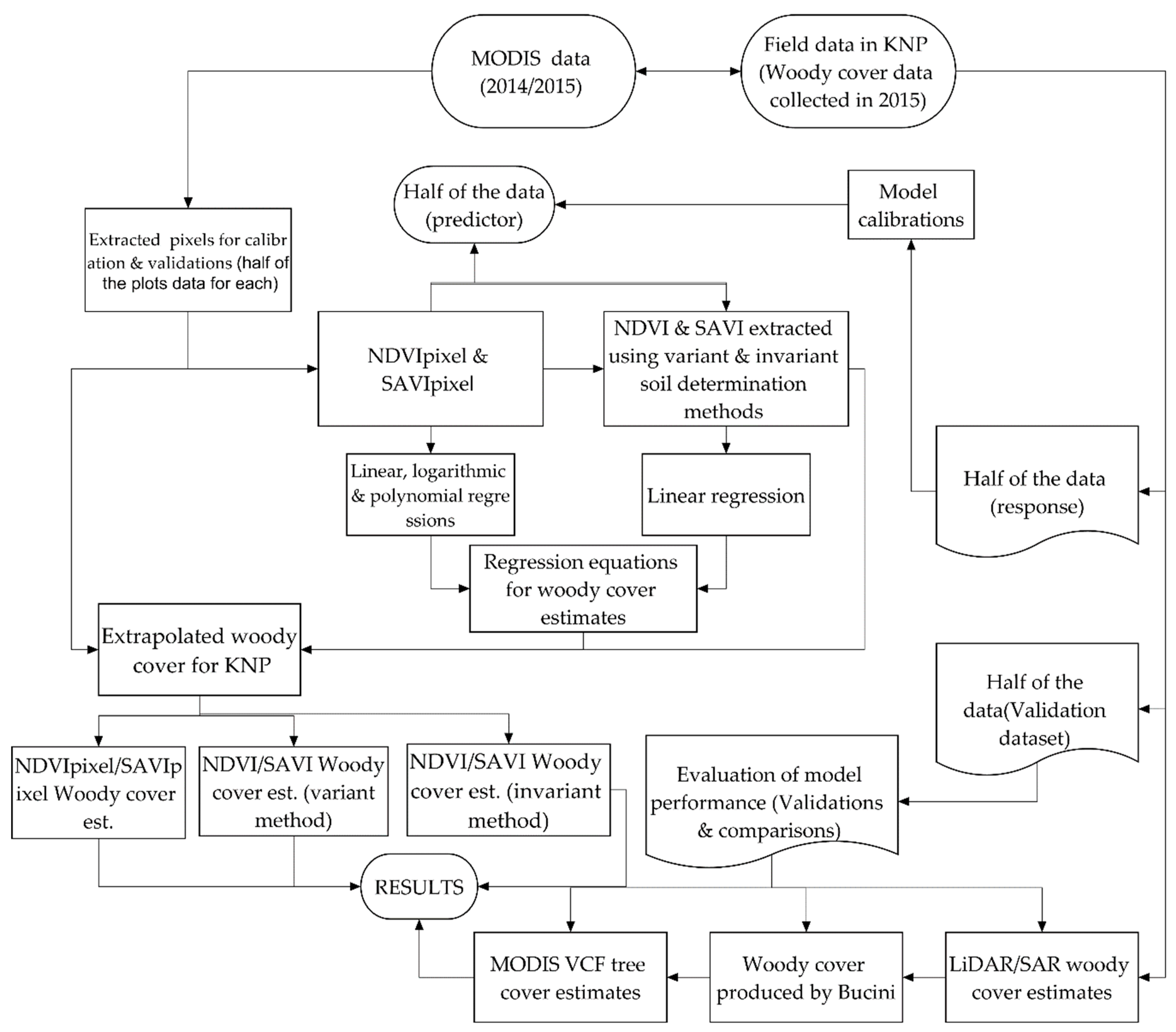
2. Materials and Methods

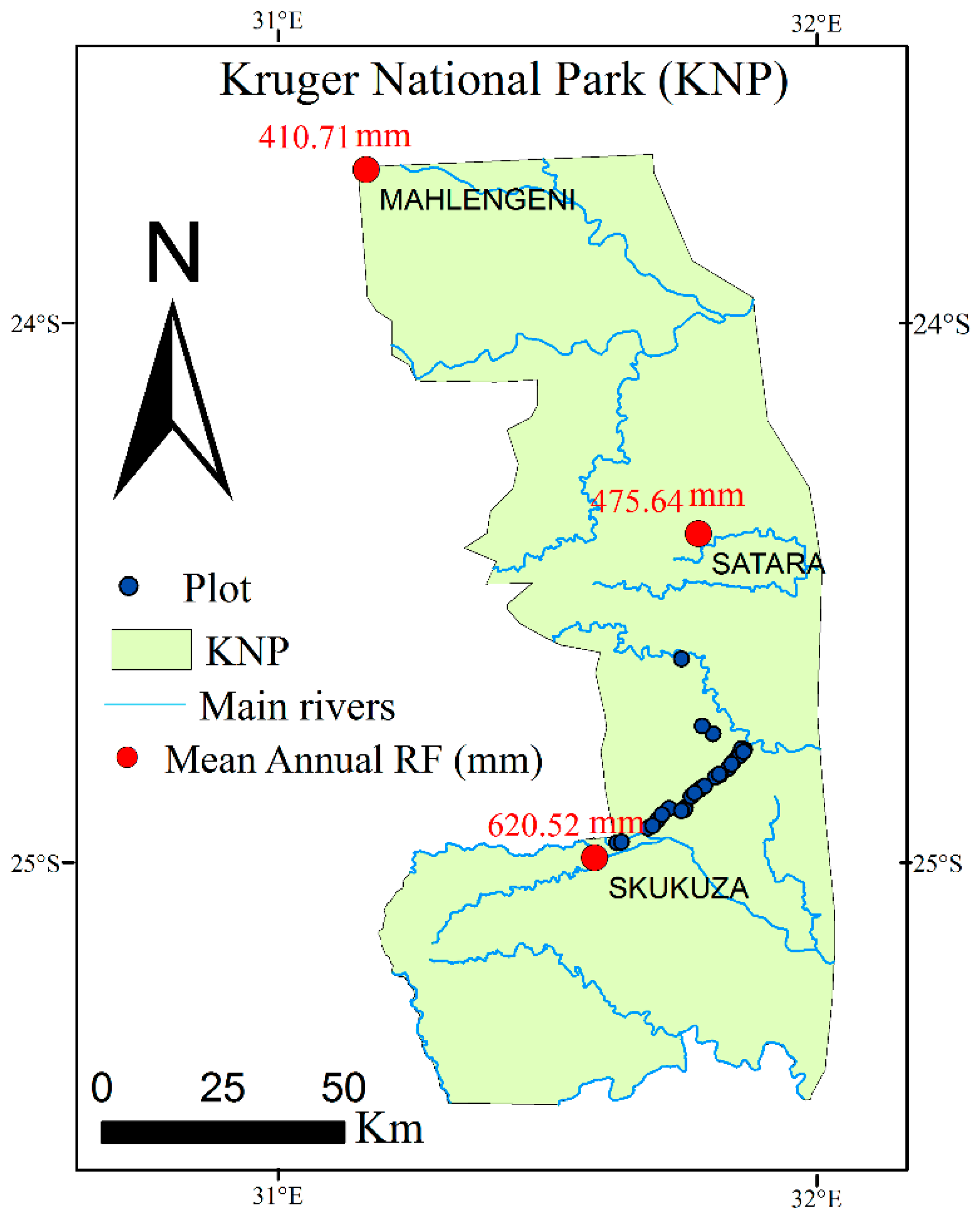
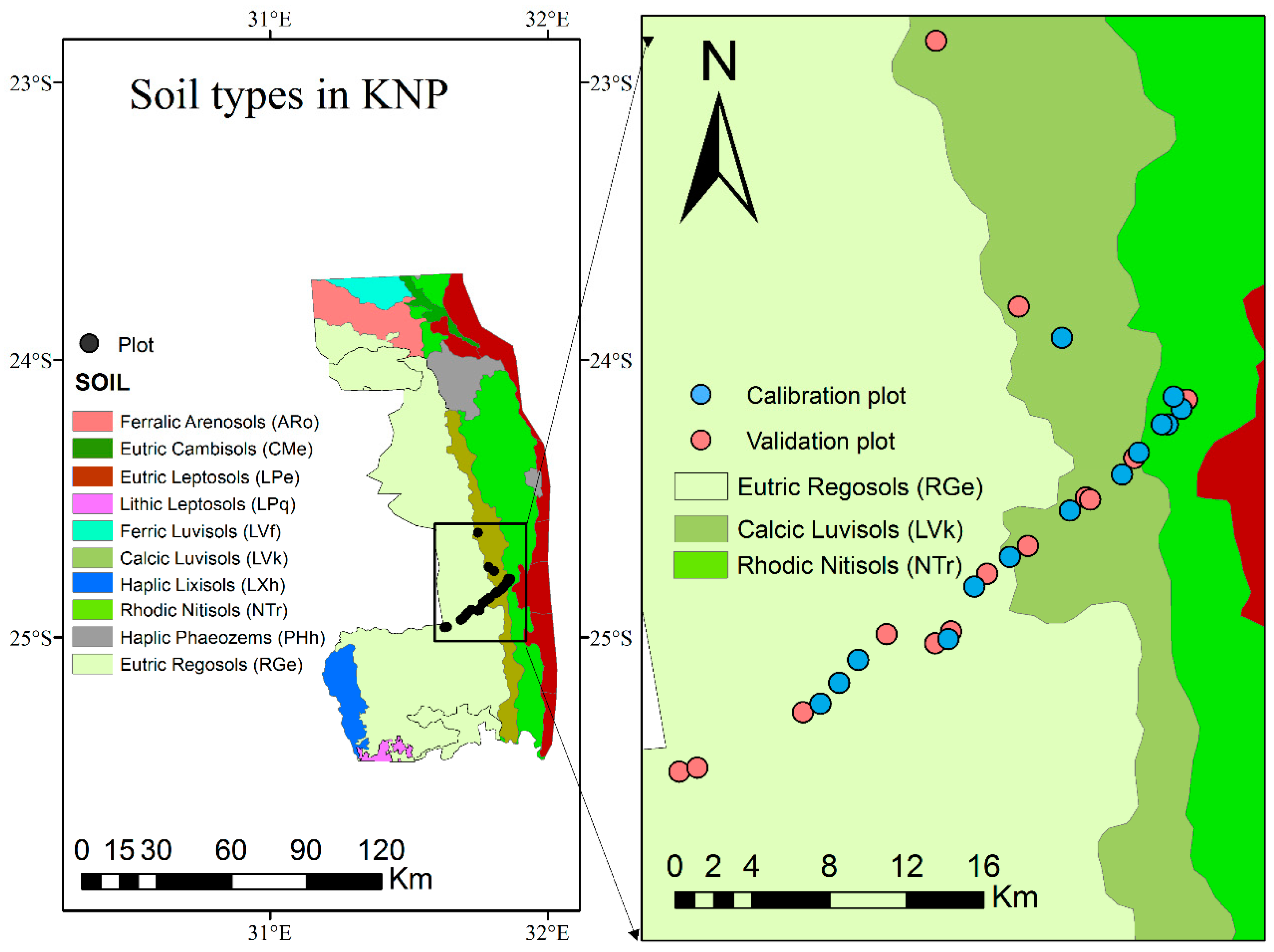
2.1. The Study Area

Kruger National Park (KNP) is South Africa’s largest nature reserve covering approximately 2,000,000 hectares. It extends 380 km from north to south and 60 km from east to west (Figure 1). Its elevation ranges from 260 m to 839 m above mean sea level. The mean annual rainfall ranges from 440 mm in the north to 750 mm in the south. Figure 1 shows the mean annual rainfall for the year 2002 to 2015 for the three weather stations in the area.

The area is divided into two main geological zones. The western part is situated on granite and the east on basaltic bedrocks [26,27,28,29,30]. Geological bedrock influences soil formation processes, and indirectly plant species and abundance distribution, and ecological processes [30]. KNP has diverse vegetation types (more than 1900 plant species) including woody and herbaceous plant functional types [27]. Figure 2 shows the soil types in KNP and the main soil types in the field plot areas based on the soil database by the International Union of Soil Sciences (IUSS), the United Nations Environment Programme, the FAO, and the International Soil Reference and Information Centre (ISRIC) [37].

The park has been classified into landscapes (e.g., Skukuza thickets, open trees, dense trees, and bush savanna) based on geomorphology, climate, soil and vegetation pattern [27,28,29]. The major woody species in the southern part include Combretum apiculatum, Acacia nigrescens, Spirostachys africana, Combretum hereroense, Sclerocarya birrea, Terminalia sericea, Combretum zeyheri, while the drier northern part is dominated by Colophospermum mopane (mopane) savanna.

2.2. Data

2.2.1. Field Data

Percent woody, herbaceous and bare soil cover were estimated for 25 field plots in the KNP during a field campaign carried out in March 2015 at the end of growing season. An ocular method proposed by Law et al. [38] was adopted for the estimation of percent cover for four structural vegetation types and bare soil within the plots (trees > 6 m, tree and shrubs 1–6 m, forbs and grasses) located along the road from Skukuza to Tshokwane (Figure 1). Three additional plots were added based on visual interpretation of Google Earth images to incorporate areas with denser tree cover than what was sampled in the field. The Google Earth imagery was acquired in May 2015. However, despite the two months difference between the field data and the Google Earth imagery, we assumed that woody phenology does not vary much within this period. Previous studies found that woody phenology is more stable over time than herbaceous phenology [28]. The field survey has considered the MODIS satellite pixel size (250 m × 250 m) by a sampling plot almost equal to the size (200 m × 200 m) of the pixel. Our observations in the field helped us to understand that vegetation cover does not vary that much over that spatial distance. The uncertainty is considered minimal. The 28 plots were placed in different vegetation types, geological conditions and soil types. Some of the tree species found in these plots include Combretum zeyheri/apiculatum (e.g., plot 14, 10, 4), Dichrostachys cinerea, Sclerocarya birrea, Terminalia sericea (e.g., plot 28), Acacia gradicortuna (e.g., plots 17, 25, and 19), Combretum hereroense (e.g., plot 19) and Albizia harveyi (e.g., plot 9). A detailed description of the field data can be found in Ibrahim et al. [26].

2.2.2. MODIS NDVI Data

MODIS NDVI data (MOD13Q1) were obtained from the National Aeronautics and Space Administration (NASA) via https://modis.ornl.gov/cgi-bin/MODIS/global/subset.pl. MOD13Q1 is a gridded level 3 product provided at 250 m spatial resolution every 16 days produced from atmospherically corrected bi-directional surface reflectance factors (BRFs) and masked for water, clouds, and cloud shadows [39,40]. A previous study developed a method based on MODIS Ross-Thick and Li-Sparse kernels to estimates of BRDF effects in NOAA-AVHRR NDVI time series. The results indicated that, in most cases, the uncorrected NDVI time series do not reflect actual seasonal and interannual variation in vegetation greenness. It was found out that the techniques reduce BRDF effects in AVHRR NDVI observations by about 50% to 85% [41]. MODIS NDVI has been used widely for retrieving vegetation composition such as vegetation structure and annual net primary productivity (ANPP) dynamics in grassland-shrub land areas [42], tree cover change [2], tree-grass separation/green-up dates [28], for monitoring vegetation and land use dynamics [43,44] and for the analysis of trends to assess the CO₂ fertilization effect on vegetation [45]. NDVI has also been used to examine the relationship between vegetation productivity and rainfall distribution along environmental gradients [43,44]. Chamaille-Jammes and Fritz [44] investigated the relationships between precipitation and primary production along a precipitation gradient. The variability of both precipitation and primary production was measured as interannual coefficient of variations (CVs), which decreased with increasing mean annual precipitation (MAP) (respectively F(1, 31) = 21,88, p, 0.0001 and F(1, 31) = 12.28, p 0.0014). The CV of annual NDVI was positively correlated with the CV of precipitation (F (1, 31) = 35.480, p, 0.0001). The study affirmed the finding of study that the sensitivity of NDVI to precipitation decreases with increasing MAP. NDVI is used here as the proxy of vegetation cover as numerous studies have identified a strong relationship between the NDVI and NPP [46,47,48]. Prince and Goward [46] designed a Global Production Efficiency Model based on the production efficiency concept. The model relies on variables (e.g., NDVI, temperature, etc.) that can be remotely sensed at global scale. It is mechanistic and does not require a correlation between NDVI and primary productivity. Moreno-de las Heras et al. [42] found the strong relationships between field net primary production (ANPP) and the annual integrals (per growing cycle) of herbaceous (R² = 0.67, p < 0.001) and shrub (R² = 0.65, p < 0.001) NDVI components. Zhu and Southworth [47] predicted NPP from the GIMMS3g NDVI data and correlated it with annual MODIS NPP stratified by savannah type. Highly significant linear correlations were found for tree savanna, bush savanna, and grassland savanna with correlation coefficients of 0.77, 0.74, and 0.80, respectively.

2.2.3. MODIS SAVI Data

The Soil Adjusted Vegetation Index (SAVI) was developed specifically to minimize soil brightness effects on vegetation indices derived from red and near-infrared (NIR) wavelengths [49]. In this study, NDVI and SAVI vegetation indices were derived from MODIS images for the period 12 July to 29 August 2014 (before the start of season) and 9 May to 26 June 2015 after the end of season. This season is best for modelling woody cover using passive optical data in savannah [50,51] because the remote sensing data for the beginning of the dry season provide the best discrimination of green woody canopies from the senesced grass layer [50,51]. The SAVI index was calculated as follows:

SAVI= (NIR − R)/(NIR + R+ L) ∗ (0.5 + L),

(1)

where the NIR is the near-infrared band, R is the red band and L stands for a soil correction factor (ranges from 0 to 1). L = 0.5 was used in this study as it has been recommended for savanna ecosystems by previous study [52].

2.2.4. MODIS Vegetation Continuous Field (VCF)

MODIS VCF is an Earth observation product describing percent tree cover, percent non-tree vegetation (mostly herbaceous) and percent bare surface and is provided globally at 250 m resolution by NASA, from the Land Processes Distribution Active Archive Centre (LP DAAC) available at http://e4ftl01.cr.usgs.gov/MOLT/. It is called MOD44B as a standard MODIS product [53,54]. The collection 5 of this product (version 0051) was used in this study, being the most recent version of this dataset at the time of writing the manuscript. Specifically, MODIS VCF for the years 2008 and 2014 were used in this study for validation and comparison purposes.

2.2.5. Validation Datasets

Two woody cover map of KNP were used as independent validation dataset. A 2010 woody cover map was produced using 14 dual-polarized (HV, HH) 12.5 m L-band ALOS PALSAR images trained with a random forest algorithm and 25,000 ha of airborne LiDAR data [55]. The L-band Synthetic Aperture Radar (SAR) data was shown to produce higher accuracy woody cover products compared to C- and X-band data in southern African savannas [56]. The LiDAR data were acquired in April 2008 (end of wet season) when woody plants were leaf-on, and the SAR images in July–August 2008 (dry season, leaf-off) to avoid soil moisture effects on the radar signal [56]. This was shown to be the best season to model woody cover in the region with SAR data [6,57]. Woody plants of at least 1 m canopy height were included. For details of the LiDAR and SAR datasets, see [56]. Validation of the SAR-map with independent LiDAR data produced an R2 = 0.8 and RMSE = 7.7% [56]. The 12.5 m LiDAR/SAR product was resampled to the 250 m MODIS resolution. In addition, the Bucini’s woody cover map was provided by Scientific Services (GIS unit) of SANParks [50,51]. The map was modelled through multiple regression techniques using a combination of optical Landsat ETM+ data, JERS-1 SAR scenes (L-band, HH polarization), and field plots of woody cover. The best predictive model was selected based on the Akaike information criterion [50,51], and the 90 m pixel size map represented woody cover conditions for the years around 2000.

2.3. Woody Cover Estimation

The data sets, approaches and the processing procedure implemented for the estimation of woody cover are summarized in Figure 3. The reference plot data from the field were used to extract the MODIS data (NDVI_pixel and SAVI_pixel). The NDVI_pixel and SAVI_pixel and invariant and variant NDVI and SAVI generated from the original data were used for model calibration using regression models. Woody cover was then extrapolated using the regression equations. The woody cover estimates were validated using the half of field data on woody cover. We validated the LiDAR/SAR, Bucini, and MODIS VCF products using our field data. We compared our estimates of woody cover with the LiDAR/SAR, Bucini, and MODIS VCF products (Figure 2). All statistical analyses were carried out in R. Detailed explanation on methods is given in the following sections.

2.3.1. Woody Cover Estimate Using NDVI_pixel and SAVI_pixel

The mean NDVI and SAVI over the dry period were calculated and taken as woody (NDVI_pixel and SAVI_pixel). In this ecosystem, woody species have two growing cycles at the time when the herbaceous layer is dormant. Grass usually dries up before the woody species lose their leaves in autumn so that two short periods with dry grass and a green woody canopy exist (before and after the wet seasons). These periods occur before and after the wet season or in autumn and spring (April–May, and October–November, respectively). The wet season starts from October and ends in April. This is considered useful in capturing the phenology of woody plants. Some woody species fully green up before the first significant rains (e.g., Sclerocarya birrea, Acacia nigrescens). Woody species in KNP usually take eight weeks to reach full leaf flush from the woody leaf-out onset. However, some woody species such as Combretum apiculatum are usually late in their leaf flush but take shorter periods to develop full leaf cover than early leaf flushers [28]. To reduce an overlap of woody and herbaceous phenology occurring probably due to a delayed start or end of season, the images chosen were for the months of July and August (12 July to 29 August 2014) before the start of season and May and June (09 May to 26 June 2015) after the end of season.

The assumption we make is that the influence of bare soil on the NDVI is minimal over a small area. The soil correction factor usually applied to derive SAVI reduces the influence of bare soil. Although both vegetation indices are sensitive to fractional vegetation cover, they are also sensitive to the soil background [4,36]. While the SAVI approach is subject to some uncertainty in woody cover estimation, the effects of soil reflectance due the nature of soil type characteristics (e.g., such as soil brightness, moisture) is likely to be negligible because of the small spatial scale being considered [58]. In addition, the soil background reflectance values are lower than the canopy reflectance due to high albedo in the tropics [33]. Jiang et al. [51] found out that the nonlinearity of NDVI over partially vegetated surfaces is more prominent with darker soil backgrounds and shadow [59].

The aim of this study is to establish the fundamental relationships between NDVI_pixel, SAVI_pixel and field data on woody cover to develop a calibration technique to assess the extent to which such relationships are able to estimate woody cover. Both linear and nonlinear regression analyses methods have been used for data calibration as the relationship between NDVI and measurements of canopy structures vary with vegetation types and seasonality [60].

2.3.2. Woody Cover Estimation Using NDVI_soil Determination Methods

In this method, it is first assumed that each pixel consists of three fractional covers: woody cover (T), bare soil cover (S), and grass cover (G). In savannas, during the dry season, most of the non-woody fraction is occupied by bare soil or dry grass while, in the wet season, green grass fractional cover makes up most of the contribution [28,61]. In the dry season, the grass layer becomes non-photosynthetic and dries up. The green grass layer (fraction of photosynthetically active vegetation) decreases from 85% to 8% while the fraction of non-photosynthetic vegetation of the same layer increases from 7% to 79% between the beginning and end of dry season [62]. Furthermore, an investigation using field reflectance measurements of bare soil, grass and woody indicated that dry grass had the lowest NDVI [62]. Hence, in this study, the non-photosynthetic grass layer was merged with bare soil. NDVI_pixel was attributed to only woody and bare soil as expressed in Equation (2). The same was applied to SAVI_pixel:

NDVI ∗ f_t + NDVI_soil ∗ (f_s + f_g) = NDVI_pixel,

(2)

where f_t is tree percent cover, f_s is fractional cover of bare soil, f_g is grass percent cover and NDVI_pixel is the mean dry season NDVI from the MODIS data.

This means that the influence of bare soil in the vegetation index does not usually allow spectral signals of vegetation to vary. To indicate the spatial variability of PFTs, the contribution of bare soil should be accounted for. Different techniques of vegetation fractional cover estimation have previously been proposed, which account for bare soil contribution. Some of these techniques are invariant to soil types and characteristics [31,32,33]. These methods rely upon the assumption that pixels with FVC = 1 and 0 exist in an image. These are described by NDVI_veg and NDVI_soil for maximum vegetation and bare soil, respectively. Hence, FVC is calculated as [63]:

$$\mathrm{FVC}=\frac{\mathrm{NDVIpixel}-\mathrm{NDVIsoil}}{\mathrm{NDVIveg}-\mathrm{NDVIsoil}}.$$

(3)

Gutman and Ignatov [31] used low spatial resolution data (0.15 × 0.15) and estimated NDVI_veg as 0.52 ± 0.03 and NDVI_soil as 0.05 ± 0.03. Similarly, Sobrino and Raissouni [32] provided a threshold NDVI_veg of 0.5 and NDVI_soil of 0.02 [35]. In this study, the methods by Zeng et al. [34] and Wu et al. [35] were adopted with slight modification due our study site being relatively small, the spatial resolution, and the fact that we lacked soil spectral reflectance field measurements [31]. The first method is invariant to soil characteristics for determining NDVI_soil. Zeng et al. [34] determined NDVI_soil by utilizing the percentile of vegetation types using the IGBP land cover classification. They used the fifth percentile of the histogram of the maximum NDVI for the barren or sparsely vegetated category as the NDVI_soil, which was 0.05, to estimate global FVC. Note, however, that only woody cover is estimated as opposed to Zeng et al. [34] whose aim was to assess statistically most likely FVC using spectra of soil collected from different datasets. Therefore, woody fractional cover is estimated as:

$$\mathrm{FVC}=\frac{\mathrm{NDVIpixel}-\mathrm{NDVIsoil}}{\mathrm{NDVIveg}-\mathrm{NDVIsoil}}.$$

(4)

The same was applied for SAVI as follows:

$$\mathrm{FVC}=\frac{\mathrm{SAVIpixel}-\mathrm{SAVIsoil}}{\mathrm{SAVIveg}-\mathrm{SAVIsoil}}.$$

(5)

The procedure requires that the histogram for each land cover is computed. Considering the size of the study area, the histogram for the whole image was computed. The minimum and maximum values of NDVI are 0.12 and 0.65. Since the maximum NDVI for this image is 0.65, a lower NDVI_soil is suggested for barren and sparsely vegetated areas. In this case, NDVI_veg and NDVI_soil are approximated as 0.02 and 0.7 for bare soil and maximum vegetation, respectively. The 0.7 is the maximum vegetation for the whole KNP. The 0.02 is the threshold for NDVI_soil. The SAVI_soil is thresholded at 0.05 and for maximum vegetation at 1.32 (the maximum for the whole KNP). However, the contribution of the NDVI_soil for each pixel has been determined from the pure pixels based on its fractional cover of bare soil. The estimation of NDVI_soil can be performed with considerable accuracy if available soil reflectance data from in situ measurements exist for the major types of soil in a given study area [4,35,36]. Unfortunately, it is challenging to acquire this information [4]. Consequently, many previous studies have relied on the Harmonized World Soil Database and IGBP land cover to assign NDVI_soil for each vegetation type, especially at regional scale [34,35].

Wu et al. [35] used the Harmonized World Soil Database (HWSD) Version 1.21 which was produced by the International Institute for Applied Systems Analysis (IIASA) and the Food and Agriculture Organization of the United Nations (FAO) to determine NDVI_soil for each soil type. The HWSD does not cover all the major soil types in KNP due to missing data from the map especially for the region of our field data. Hence, a global soil and terrain database at a scale of 1:1 million developed by the International Union of Soil Sciences (IUSS), the United Nations Environment Programme, the FAO, and the International Soil Reference and Information Centre (ISRIC) [37] was used here. Based on Wu et al. [35], the NDVI_soil for the three types of soil in our plot locations (which include Regosols, Luvisols, and Nitisols) were thresholded at 0.21, 0.24, and 0.32, respectively. This approach slightly differs from Wu et al. [35]. First, a linear method is applied as opposed to Wu et al. [35]. Given the small size of the study area, NDVI_soil is considered for each soil type and for each plot, while a single value for maximum NDVI (NDVI_veg) was considered for all locations. For the NDVI, Regosols, Luvisols, and Nitisols have been thresholded at 0.015, 0.02, and 0.02, respectively, while, for SAVI, the thresholds were 0.04, 0.05, and 0.06. The three types of soils are described based on the World Reference for Soil Resources (2014) according to the International Soil Classification System of the Food and Agriculture Organization (FAO) of the United Nations [64]. Regosols are characterised as the very weakly developed mineral soils in unconsolidated materials that do not have a mollic or umbric horizon. They are generally fine-grained material and are particularly common in semi/arid areas [64]. Luvisols have a higher clay content in the subsoil than in the topsoil, as a result of pedogenetic processes (especially clay migration) leading to an argic subsoil horizon [64]. Nitisols are deep, well-drained, red tropical soils with diffuse horizon boundaries and a subsurface horizon with at least 30 percent clay. Nitisols are some of the most productive red tropical soils [64].

2.4. Regression Analyses

In this study, different types of regression models were used to assess the relationship between the percent woody cover from the field campaign in 2015 and the independent variables (NDVI or SAVI vegetation index). Only 50% of the field data on woody cover (14 plots) was used for model calibration while holding the remaining 50% back for validation. The power of our study design was assessed by using the Power and Sample Size Calculation software provided by Dupont et al. [65]. In this study, with reference to sample size (14 plots), we found statistical power following Dupont et al. [65] methods for sample size and power calculations. Our sample size results in a statistical power of 0.98. The type of regression analysis depends on the nature of the phenology metric being used. The procedure assumes that the NDVI-fractional vegetation cover relationship (or SAVI) is a function of vegetation type, the influence of understory and bare soil [60,66,67,68]. The regression model applied for each phenology metrics is explained below:

(1) Since the assumption to use the mean of the images of chosen MODIS data (NDVI_pixel and SAVI_pixel) does not preclude the presence of bare soil, different regression models were tested for estimating woody cover. Although it has previously been reported that the relationship between vegetation indices (especially NDVI) and percent cover depends largely on vegetation type [60], or may even have a strong linear relationship with sparse vegetation [66,67], it is not well known how the relationship with woody cover would be in KNP. Therefore, simple linear, polynomial and logarithmic models were tested for both vegetation indices to find the best fit for percent woody cover estimation.

(2) Only a simple linear regression was applied to NDVI_soil and SAVI_soil determination methods.

2.5. Assessment of Model Performance

The assessment of model performance for fractional woody cover from the MODIS NDVI/SAVI time series data uses the remaining field plot data (14 plots) not used for calibration. The LiDAR/SAR-based woody cover map and the MODIS VCF datasets were first compared to the field observations to quantify their accuracies. The validation of MODIS VCF with field data uses the MODIS VCF data for the year 2014 since the field campaign was in 2015. To assess model performance for woody cover estimated in this study, the coefficient of determination (R²) of the regression model was used to measure the strength of the relationship between the predicted and the observed values. The predicted data for each model are taken as the independent variable and the observed as the dependent [69]. In addition, RMSE was used to determine the goodness-of-fit. All MODIS NDVI/SAVI woody cover estimates were validated with field data are from year 2014/15.

2.6. Comparison of Woody Cover Estimates with LiDAR/SAR and Bucini Woody Cover Maps

The Pearson correlation coefficient is the measure of the bidirectional linear correlation between two variables and was used to assess whether woody cover estimates from this study as well as the MODIS VCF product are related to the LiDAR/SAR and Bucini woody cover maps. The significance of the relationship was also assessed at alpha = 0.05.

3. Results

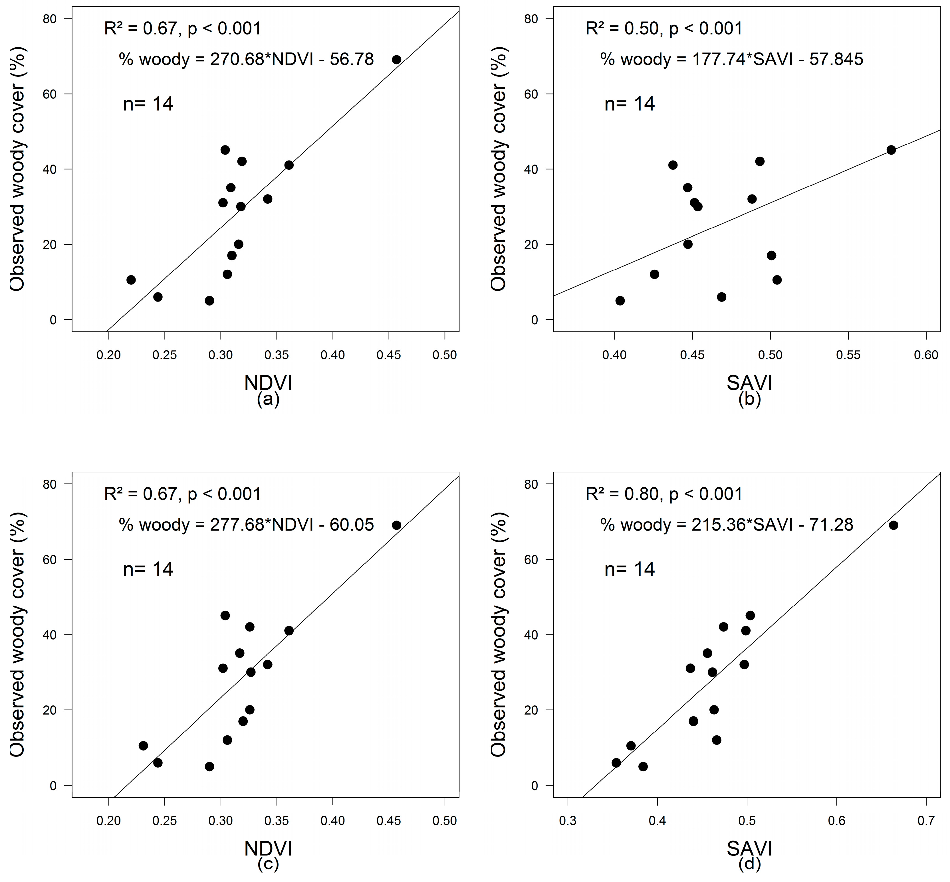
3.1. Model Calibration

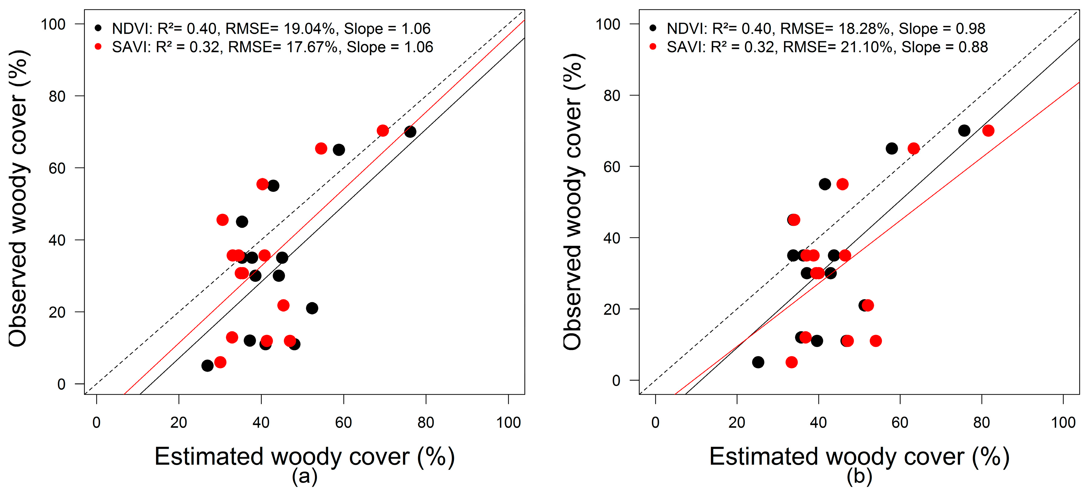
3.1.1. NDVI_pixel and SAVI_pixel for Woody Cover Estimate

Data on woody and herbaceous cover, and NDVIpixel and SAVIpixel used for woody cover estimation are shown in

Table 1. Woody, grass, bare soil, NDVI_pixel and SAVI_pixel for woody cover estimation.

Plot	Woody Cover	Grass Cover	Bare Soil	NDVIpixel	SAVIpixel
1	5	85	10	0.336	0.485
3	6	85	9	0.289	0.454
4	10.5	45	44.5	0.264	0.434
7	12	67	21	0.3492	0.544
9	17	78	5	0.349	0.499
10	20	70	10	0.3547	0.520
12	30	45	25	0.352	0.511
15	31	55	14	0.335	0.498
16	32	35	33	0.375	0.557
19	35	22	43	0.341	0.502
21	41	35	24	0.389	0.551
22	42	30	28	0.346	0.515
24	45	45	10	0.330	0.562
27	69	20	11	0.471	0.691

. Figure 4 shows the relationship between NDVI_pixel and SAVI_pixel and percent woody cover surveyed during the 2015 field campaign. The NDVI_pixel versus the percent tree cover (Figure 4a,c,e) had moderate coefficient of determination with R² between 0.53–0.58 and p < 0.01. The relationships for linear and polynomial regressions yielded the strongest fits (R² = 0.56, p < 0.01 and R² = 0.58, p < 0.01. Although the difference between linear and nonlinear regression (Figure 4e: R² = 0.53, p < 0.01) is not important, the nonlinearity of the NDVI increases with increasing species composition. In the dry season, the woody species are active while other PFTs (e.g., grasses) are dry making NDVI more sensitive to vegetation. The accuracy of SAVI_pixel is higher (Figure 4b,d,f) than that of NDVI_pixel with R² = 0.56 to 0.67 (p < 0.01). The saturation of NDVI_pixel occurs at a higher percent cover than that of SAVI_pixel. This is expected since SAVI applied correction factors, which minimise the effect of the soil background. Overall, the existing relationship between the NDVI_pixel, SAVI_pixel with percent woody cover implies that they can both be used to estimate percent woody cover.

3.1.2. NDVI and SAVI for Woody Cover Estimation with NDVI_soil Determination Using a Modified Procedure by Zeng et al. [34] and Wu et al. [35]

Table 2. Estimates of percent cover using NDVI and SAVI with soil determining methods using a modified procedure by Zeng et al. [34] and Wu et al. [35]

Plot	Woody Cover	Grass Cover	Bare Soil	Grass & Bare Soil	Soil Types	NDVIpixel	NDVIZeng	NDVIWu	SAVIpixel	NDVIZeng	NDVIWu
1	5	85	10	95	Nitisols	0.336	0.290	0.290	0.485	0.404	0.384
3	6	85	9	94	Nitisols	0.289	0.244	0.244	0.454	0.469	0.354
4	10.5	45	44.5	89.5	Regosols	0.263	0.220	0.231	0.434	0.504	0.371
7	12	67	21	88	Luvisols	0.349	0.306	0.306	0.544	0.426	0.466
9	17	78	5	83	Regosols	0.349	0.310	0.320	0.499	0.501	0.440
10	20	70	10	80	Regosols	0.354	0.316	0.326	0.520	0.447	0.463
12	30	45	25	70	Regosols	0.352	0.318	0.327	0.511	0.454	0.461
15	31	55	14	69	Luvisols	0.335	0.302	0.302	0.498	0.451	0.437
16	32	35	33	68	Luvisols	0.375	0.342	0.342	0.557	0.488	0.497
19	35	22	43	65	Regosols	0.340	0.309	0.317	0.502	0.447	0.456
21	41	35	24	59	Luvisols	0.389	0.361	0.361	0.551	0.438	0.499
22	42	30	28	58	Regosols	0.346	0.319	0.326	0.515	0.493	0.474
24	45	45	10	55	Nitisols	0.330	0.304	0.304	0.562	0.578	0.504
27	69	20	11	31	Luvisols	0.471	0.457	0.457	0.691	0.683	0.664

shows the field plots data for the percent woody, herbaceous, bare soil and the type of soil for each calibration plot. Table 2 also indicates the fraction of the NDVI (NDVI_Zeng and NDVI_Wu) and SAVI (SAVI_Zeng and SAVI_Wu) estimated using the two soil background effect correction methods. Figure 5a–d shows the calibration results for NDVI and SAVI. NDVI estimates for both methods show an increased accuracy much better than when NDVI_soil is not removed. The invariant method for which an NDVI_soil threshold of 0.02 was used has a strong relationship with percent woody cover: R² = 0.67, p < 0.01 (Figure 5a) while the other approach which considered the Harmonized World Soil Database to determine the NDVI_soil for each soil type in the plot locations also had a strong relationship with percent cover (R² = 0.67, p < 0.01, Figure 5c). There is a slight difference between the two vegetation indices as only three types of soil were found in the plot locations based on the soil database.

The invariant soil determining method for SAVI_Zeng which threshold NDVI_soil at 0.05, is not very effective as its accuracy (R² = 0.50, p < 0.01) is slightly lower than the initial relationship for which the soil contribution is unaccounted. This means that the invariant method applied here may be less accurate in inferring woody cover compared to other approaches though validation results might show otherwise, while, when considering the soil type in determining the NDVI_soil, a strong relationship is observed between the SAVI_Wu and percent woody cover (R² = 0.80, p < 0.01). In this case, the NDVI_soil 0.04 was threshold for Regosols while Luvisols and Nitisols at 0.05 and 0.06, respectively. Overall, all vegetation indices have shown a good relationship with the percent woody cover.

3.2. Comparison of LiDAR/SAR, Bucini and MODIS VCF Woody Cover with Field Data at Plot Level

LiDAR/SAR, Bucini and MODIS VCF woody cover estimates were assessed with field observations collected (28 plots) in 2015 (Figure 6). The assessment with field estimates indicates that the LiDAR/SAR woody cover map has the highest accuracy (R² = 0.45, p < 0.001, Slope = 0.5, RMSE = 15.90%) followed by Bucini (R² = 0.55; p < 0.001, Slope = 0.5, RMSE = 17.54%) compared to MODIS VCF (R² = 0.53, p < 0.001, Slope = 0.05, RMSE = 27.5%). The difference between these woody cover estimates is more obvious in the RMSE and Slope (Figure 6).

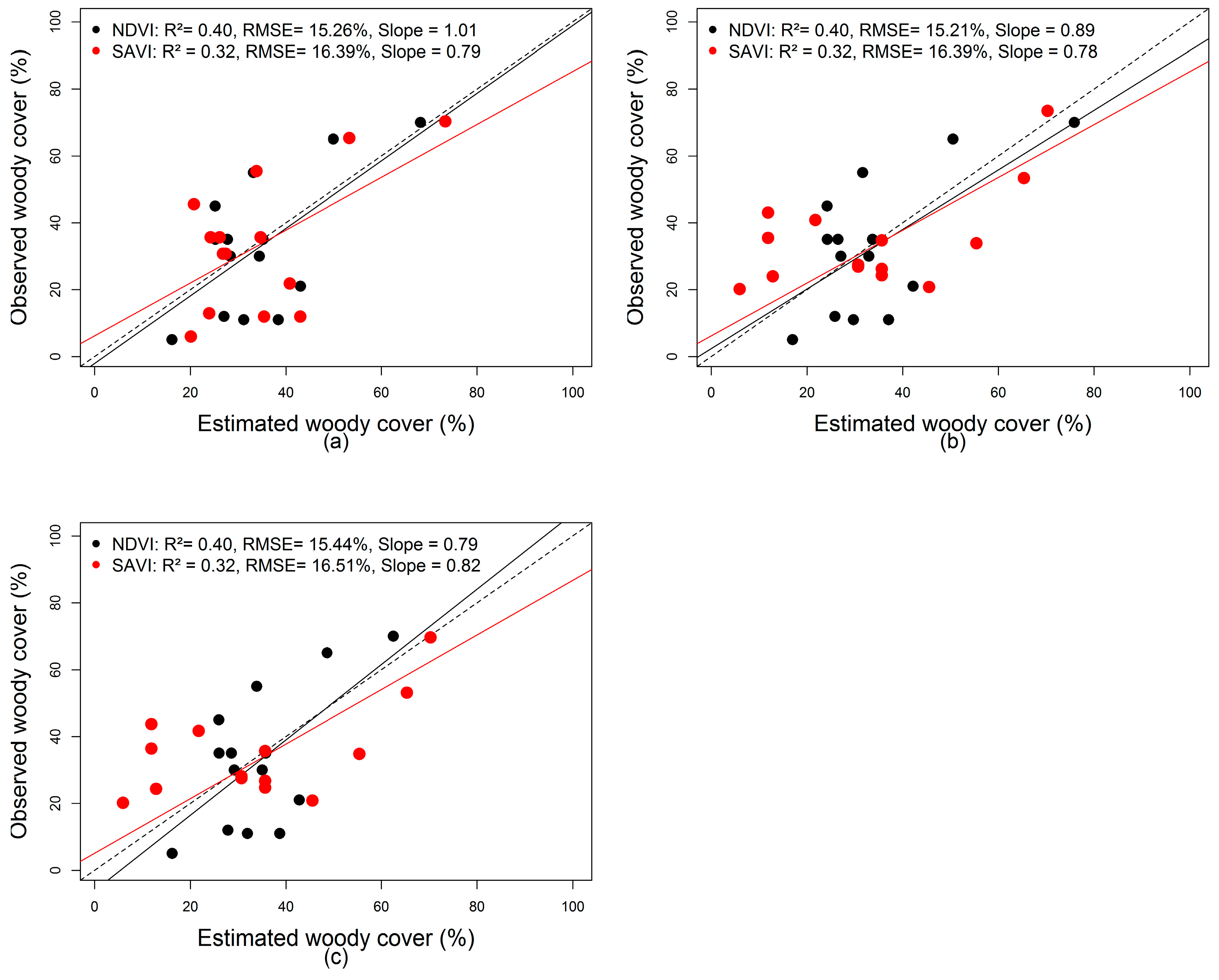
3.3. Validation of Woody Cover Estimates

3.3.1. MODIS NDVI_pixel and SAVI_pixel Woody Cover Maps

Table 3. Validation of MODIS NDVI_pixel and SAVI_pixel woody cover estimates.

Plot No.	Woody Cover (%)	NDVIpixel	SAVIpixel	NDVIpixel Estimated Woody Cover			SAVIpixel Estimated Woody Cover
				Linear	Polynomial	Logarithmic	Linear	Polynomial	Logarithmic
2	5	0.307	0.486	16.17	16.99	16.24	19.35	19.35	19.32
5	11	0.359	0.550	31.21	29.74	31.98	34.80	34.78	35.73
6	11	0.385	0.582	38.42	37.07	38.71	42.43	42.41	43.14
8	12	0.345	0.502	27.08	25.88	27.89	23.19	23.19	23.59
11	21	0.401	0.573	43.04	42.20	42.80	40.23	40.21	41.04
13	30	0.371	0.517	34.47	32.95	35.08	26.69	26.68	27.37
14	30	0.350	0.514	28.41	27.10	29.23	26.13	26.12	26.77
17	35	0.347	0.511	27.78	26.52	28.60	25.41	25.40	26.00
18	35	0.374	0.547	35.24	33.74	35.80	34.08	34.06	35.00
20	35	0.338	0.503	25.26	24.27	26.04	23.50	23.50	23.93
23	45	0.338	0.489	25.22	24.24	26.01	19.99	19.99	20.03
25	55	0.366	0.544	33.20	31.68	33.88	33.19	33.17	34.11
26	65	0.425	0.625	49.99	50.53	48.65	52.84	52.84	52.62
28	70	0.489	0.710	68.22	75.92	62.53	73.12	73.17	69.35

shows field validation plots and NDVI_pixel, SAVI_pixel as well their corresponding woody cover estimated from simple linear, polynomial and logarithmic regression equations. Figure 7a,c presents an accuracy assessment of woody cover from the NDVI_pixel and SAVI_pixel (mean of dry season images for 2014/2015) using the field data from 2015. The estimated woody cover using linear regression has an R² = 0.40, p < 0.01, slope = 1.01 for NDVI_pixel, RMSE = 15.26% and R² = 0.32, p < 0.03, slope = 0.79, RMSE = 16.39% for SAVI_pixel. The level of accuracy for NDVI_pixel and SAVI_pixel with polynomial regression are not far from the simple linear regression (NDVI_pixel: R² = 0.40, p < 0.01, slope = 0.89, RMSE = 15.21%; SAVI_pixel: R² = 0.32, p < 0.03, slope = 0.78, RMSE = 15.39%). The logarithmic model is slightly less accurate for both vegetation indices (NDVI_pixel: R² = 0.40, p < 0.01, slope = 0.79, RMSE = 15.44%; SAVI_pixel: R² = 0.32, p < 0.03, slope = 0.82, RMSE = 16.51%). These results suggest that both NDVI_pixel and SAVI_pixel are sensitive to percent woody cover. However, with reference to the scatterplots (Figure 7a,c), the nonlinearity of the two relationships is evident.

3.3.2. NDVI and SAVI Woody Cover Estimation from the NDVI_soil Determination Methods by Zeng et al. [34] and Wu et al. [35]

Table 4. Validation of MODIS NDVI woody cover maps estimated using two methods of soil signal removal.

Plot No.	Observe Woody Cover (%)	NDVIpixel	SAVIpixel	Estimated Woody Cover (%) (Zeng et al.)	Estimated Woody Cover (%) (Wu et al.)	Estimated Woody Cover (%) (Zeng et al.)	Estimated Eoody Cover (%) (Wu et al.)
2.00	5.00	0.307	0.486	28.52	28.99	29.382	33.39
5.00	11.00	0.359	0.550	39.94	43.83	40.757	47.17
6.00	11.00	0.385	0.582	45.57	51.16	46.445	54.06
8.00	12.00	0.345	0.502	31.36	32.68	32.225	36.83
11.00	21.00	0.401	0.573	43.95	49.05	44.845	52.12
13.00	30.00	0.371	0.517	33.94	36.04	34.892	40.06
14.00	30.00	0.350	0.514	33.53	35.50	34.358	39.42
17.00	35.00	0.347	0.511	33.00	34.81	33.825	38.77
18.00	35.00	0.374	0.547	39.40	43.14	40.224	46.52
20.00	35.00	0.338	0.503	31.59	32.98	32.403	37.05
23.00	45.00	0.338	0.489	28.99	29.60	29.915	34.03
25.00	55.00	0.366	0.544	38.75	42.29	39.691	45.88
26.00	65.00	0.425	0.625	53.27	61.17	54.088	63.32
28.00	70.00	0.489	0.710	68.25	80.65	69.195	81.63

shows field validation plots and their corresponding woody cover estimated using two approaches which account for NDVI_soil and SAVI_soil in the estimation. Figure 8a shows the validation of woody cover estimates from a modified procedure of vegetation fractional cover estimation by Zeng et al. [34] for NDVI (Figure 8a) (R² = 0.40, p < 0.01, slope = 1.06; RMSE = 19.04%) as well as for SAVI (Figure 8a) (R² = 0.32, p < 0.3, slope = 1.06; RMSE = 17.34%). The woody cover estimated for both vegetation indices using Zeng’s procedure indicated that the approach can be used to infer woody fractional cover using dry season images even though the accuracy of the estimated woody cover were slightly lower than when NDVI_soil were unaccounted for. There is an overestimation of woody cover in the lower percent cover where the contribution of soil is higher demonstrating the implication of an invariant NDVI_soil removal approach. Figure 8b shows the validation of woody cover estimated from the modified procedure of vegetation fractional cover estimates by Wu et al. [35] (NDVI: R² = 0.40, p < 0.01, slope = 0.98; RMSE = 18.28%, SAVI: R² = 0.32, p < 0.02, slope = 0.88; RMSE = 19.17%). The accuracy of this approach is slightly higher than for the previous method. The difference between the two methods is more obvious in the RMSE and slope demonstrating the importance of the NDVI_soil determination method that considers soil type characteristics.

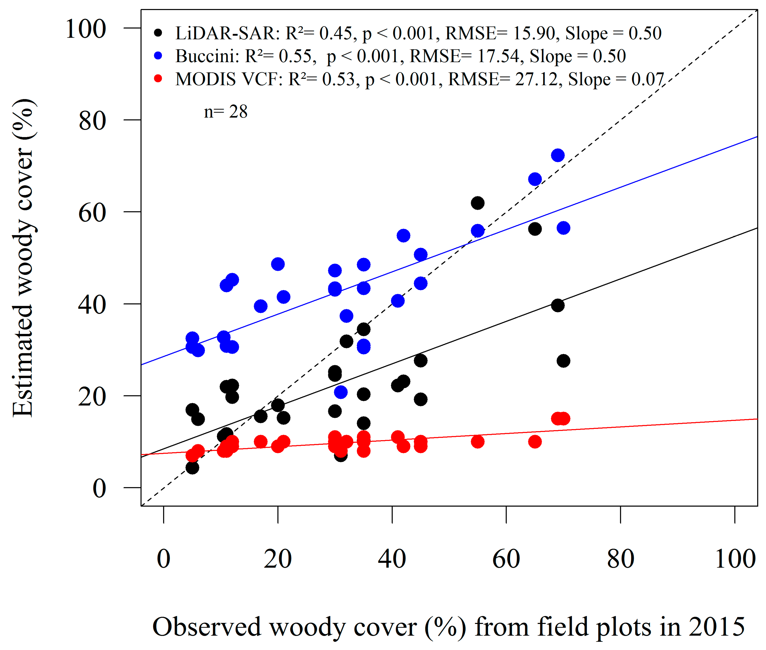
3.3.3. Comparison of Estimated Woody Cover with LiDAR/SAR-Derived and Bucini’s Woody Cover Estimates Using Pearson Correlation Analysis and RMSE

Table 5. Correlation and RMSE of estimated woody cover with LiDAR/SAR and Bucini estimates.

Woody Cover Estimates	LiDAR/SAR 2008			Bucini 2001
	r	p-Value	RMSE (%)	r	p-Value	RMSE
NDVIpixel (Linear)	0.52	0.05	16.46	0.63	0.014	15.15
NDVIpixel (Polynomial)	0.49	0.07	17.14	0.62	0.016	15.98
NDVIpixel (Logarithmic)	0.52	0.05	15.99	0.63	0.014	14.93
NDVI (Zeng’s et al.)	0.52	0.05	19.28	0.59	0.02	12.85
NDVI (Wu et al.)	0.52	0.05	22.85	0.59	0.02	12.78
SAVIpixel (Linear)	0.53	0.05	16.74	0.59	0.02	16.66
SAVIpixel (Polynomial)	0.53	0.05	16.74	0.59	0.02	16.67
SAVIpixel (Logarithmic)	0.53	0.05	16.42	0.58	0.02	16.28
SAVI (Zeng’s et al.)	0.52	0.05	19.94	0.59	0.02	12.51
SAVI (Wu et al.)	0.52	0.05	25.49	0.59	0.02	12.50
MODIS VCF	0.39	0.16	23.36	0.40	0.17	40.83

presents a correlation coefficient and RMSE of NDVI, SAVI, and MODIS VCF tree cover estimates with LiDAR/SAR and Bucini using 14 validation plots from the field campaign in 2015. All vegetation indices have a significant relationship with previous tree cover estimates except the polynomial model in NDVI_pixel with LiDAR/SAR. The linear model had the highest correlation for both vegetation indices (NDVI_pixel: r = 0.52, p = 0.05 with LiDAR/SAR and r = 0.63, p = 0.014 with Bucini; SAVI_pixel: r = 0.53, p = 0.05 with LiDAR/SAR and r = 0.59, p = 0.02 with Bucini). However, the logarithmic model recorded the lowest RMSE in both NDVI_pixel (RMSE = 15.99) and SAVI_pixel (RMSE = 14.93) compared to linear (NDVI_pixel: RMSE= 16.46 and SAVI_pixel: RMSE = 15.15) and polynomial models (NDVI_pixel; RMSE = 17.14 and SAVI_pixel: RMSE = 15.98). The correlation between MODIS VCF with the previous tree cover estimates is however not significant r = 0.39, p = 0.16, RMSE = 23.36 with LiDAR/SAR and r = 0.40, p = 0.17, RMSE = 40.83 with Bucini) and had higher RMSE.

4. Discussion

4.1. Comparison of LiDAR/SAR, Bucini and MODIS VCF Data

The previous products on woody cover have been validated by the providers and were found relatively accurate. The LiDAR/SAR and Bucini woody cover map have been found the most accurate using our field data (Figure 6). Despite the differences between the times of field campaign data that were used for this study (2015), the LiDAR/SAR and Bucini [48] woody cover maps are consistent with our field measurements (Figure 6). Although LiDAR/SAR woody cover has an advantage since LiDAR has the ability to measure vegetation in three dimensions [29,70], another important consideration is acquiring the SAR images in July–August 2008 (dry season, leaf-off) to avoid soil moisture effects on the radar signal [6]. The Bucini woody cover map was produced from the synergy between optical (Landsat ETM+ and JER-S) and SAR data. The accuracy of this product might result due to consideration of phenology of woody species (dry season images for the optical dataset to maximize discrimination of woody vegetation) as well as for accounting the effects of climate, soil characteristics, topography, fire frequency and herbivory in a regression analysis to estimate woody cover.

Despite reported strengths of MODIS VCF datasets observed in many studies [9,70,71,72], the accuracy of the products is lower in savannas, particularly when certain statistical observations are put into consideration. The accuracy of MODIS VCF has the highest RMSE (28.6%) of all datasets compared here, probably due its model calibration, which only considered cover of trees taller than 5 m (Figure 6). This simply means that there is an underestimation of tree or woody cover from the MODIS VCF in this region where many trees are lower than 5 m. The underestimation of woody cover from the MODIS VCF compared to in situ data observed here is similar to the study by Brandt et al. [3], whose estimate of woody cover in the Sahel was nine times higher than the MODIS VCF. Consequently, low accuracy of MODIS VCF as a proxy for overall woody cover has been reported in the scientific literature [7,25,73].

The use of a large number of phenology metrics acquired in different periods regardless of vegetation dynamics [72,74], the presence of bad pixels (haze, cloud cover and shadow), the training datasets (regression tree usually require large samples), and limitations inherent in the MODIS viewing geometry (the effects is more with the individual bands than the vegetation index-NDVI) may be responsible for the limitations of the MODIS VCF in savannas. None of the MODIS VCF (2014) pixel values was of bad quality within the field plots used for this study. Consideration of the seasonal vegetation dynamics is useful for global scale mapping of woody cover in savannas using space observations. This is due to large differences in vegetation phenology during the wet and dry seasons [75] and consequent limitations such as cloud cover and sensor viewing geometry, which may affect the interannual and seasonal variation of woody/herbaceous phenology [41,76].

4.2. The NDVI_pixel and SAVI_pixel

The composite dry season images used for vegetation indices to estimate woody cover in KNP were accurate (Figure 7a–c). The validation of woody cover estimated from the NDVI showed a lower error (RMSE = 15.26%, 15.21%, 15.44% for the linear, polynomial and logarithmic model respectively) for all models compared to SAVI_pixel (RMSE = 16.39%, 16.39%, 16.51% for linear, polynomial and logarithmic model, respectively) (Figure 7a–c), illustrating the strong dependence of NDVI on woody canopy structure during the dry season in KNP. This also demonstrated the presence of a photosynthetically active woody layer in the dry season as previously observed [50]. The relationship between the NDVI and PFT types depends on the nature of the ecosystem in question [33,41,60].

The relationship between NDVI_pixel / SAVI_pixel and percent woody cover is approximately linear (Figure 7a). Most of the plots used for woody cover in this study are within the granitic zone, where soil types differ from the basaltic zone. The results discussed in this section agree with previous studies [60,66,67]. A recent study found a linear relationship between FVC and the EVI as well as the SAVI vegetation index. In the same study, the relationship between the NDVI and FVC was nonlinear due to saturation effects at high vegetation fractions, the presence of shadow as well as the influence of soil background [77].

There is strong correlation between SAVI_pixel / NDVI_pixel and Bucini / LiDAR/SAR woody cover (Table 5). At the lower percent woody cover, the points are clustered. This demonstrated the influence of radiative transfer from the surface on canopy reflectance especially where there is mixed woody, herbaceous and bare soil fractions [70,78,79,80]. Therefore, in a sparse vegetation cover, radiative interactions cause soil to be prominent and canopy visible reflectance will contain a strong backscatter component. The soil reflectance effect is less prominent in the NIR canopy reflectance, since multiple scattering of NIR radiation by vegetative components dominate. Hence, the influences of soil reflectance reduces with decreasing canopy gaps [36,81].

4.3. Woody Cover Estimated Using Two NDVI_soil and SAVI_soil Determination Methods

The assessment of woody cover maps from the soil determination methods indicated a moderate linear relationship between the predicted and observed percent woody cover (Figure 8a,c). Although the slope of the regression line for both vegetation indices were higher (slope ranges from 0.88 to 1) (Figure 8a,c) compared to woody cover estimates without removal of the soil signal (slope ranges from 0.78 to 1) (Figure 8a), the RMSE is still high with soil determination methods. The RMSE for woody cover estimates without soil signal removal ranges between 15.21–16.51%. In contrast, the RMSE for the invariant method is 19.04% and 17.34% for the NDVI and SAVI vegetation indices estimates, respectively, while the RMSE for the variant method is 18.28% and 19.17% for the NDVI and SAVI estimates, respectively. Therefore, RMSE increases to more than 3% for the NDVI and about 5% for SAVI. The RMSE for SAVI vegetation index increases to about 2% with an invariant method and 4% with variant method. The SAVI vegetation index was found to be less sensitive to soil signal removal than the NDVI. SAVI is one of the vegetation indices specifically developed to reduce soil backgrounds effects. Although soil colour is useful for differentiating soil reflectance [80], soil moisture was considered an important factor in influencing vegetation indices [82]. From the results in Figure 8, uncertainty in the estimates of percent woody cover at lower cover is high in all methods. The second approach of the soil determination methods overestimated low percent woody cover values. This can be explained by the sensitivity of the canopy NDVI or SAVI to soil background or the result of changing canopy structure, which might decrease in the NIR reflectance and increasing visible reflectance consequently leading to reduced NDVI. In addition, the sensitivity of vegetation indices to soil backgrounds was found to be greatest in the intermediate level of vegetation cover [36,83]. It is usual to overestimate percent woody cover whenever soil contribution is underestimated and vice versa [4]. Overall, despite the uncertainty in the estimation of percent woody cover with the soil determination approaches used in this study, heterogeneity is present in the woody cover estimates derived from these approaches.

4.4. The Uncertainties and Sources of Errors and Proposed Improvements

While our results demonstrated the potential of MODIS data to estimate percent woody cover from vegetation indices, woody cover estimated in this study has some limitations and remaining uncertainties that must be considered:

(1) Phenology

Phenology of PFTs in savannas is usually influenced by many environmental factors [84] Specifically, woody phenology is influenced mainly by temperature and day length [85], or precipitation and disturbance in certain conditions [86]. For these reasons, the estimates of percent woody cover from passive optical remote sensing are less accurate compared to high-resolution datasets. While high resolution data such as LiDAR (active optical data) can determine woody canopy cover by measuring its 3D structure, the estimates from the passive optical imaging datasets mostly rely on the green canopy cover within a pixel [3].

The grass layer (fraction of photosynthetic vegetation) in savannas may have changed from 85% to 8% and the fraction of non-photosynthetic vegetation of the same layer may increase from 7% to 79% between the beginning and end of dry season [62]. Although careful attention was given to defining the dry season, woody/herbaceous cover separation can be affected by certain grass species that are supported by soil moisture and temperature [28]. In savannas, certain environmental factors favor grass growth and influence its phenology, productivity and biomass allocation [87,88]. Temperature and soil moisture are generally not limiting factors of grass productivity in KNP [28]. This might contribute to the overestimation of woody cover, especially in a highly mixed woody/herbaceous area. In addition, the time differences between the LiDAR/SAR, Bucini, and field data campaign may affect the accuracy assessment of the two products from MODIS compared here. Although the MODIS vegetation indices (e.g., NDVI) are less sensitive to illumination than individual bands, as previously reported in the literature, the estimates of woody cover in this study may well contain remaining uncertainties despite being specific to a particular season [41,76]. The temporal granularity of the MODIS NDVI products of 16 days limits the temporal precision of the detection of changes in greenness. Denser time-series data would be preferable.

(2) The ground data (field plot data on percent woody/herbaceous cover)

The calibration data used in our models may not be the representative of all species over the KNP landscape. The field method for woody cover estimation is a visual approach which may also constrain the accuracy of our models due to remaining uncertainties in the field data collection. However, the results presented in this study demonstrated that percent woody cover can be estimated from vegetation indices in savannas, and that a single regression model based on our field data indicated RMSE between 15–21%. However, while the accuracy assessment indicates lower errors, percent woody cover of <40%, where spectral signatures are probably dominated by understorey (dry grass) and soil, is not highly correlated with the field measurements. This might arise due to the presence of soil and dry grass, underestimation of percent woody cover in the field campaign or changes in woody phenology due to fire over the period [89]. For both calibration and validation plots, there are only a few plots with percent woody cover >40%. This means that, if the regression models are to be developed and applied consistently over the large area, it is important that they are established on a much larger sample than as presented in the current study. This may reduce uncertainty and increase model accuracy.

(3) NDVI_soil estimation

The use of in situ measurements of soil reflectance remains a crucial step for an effective determination of NDVI_soil in a pixel to estimate woody cover fraction [4,82,90], especially in savannas where the availability of vegetation indices at MODIS resolution of 250 m is essential for capturing vegetation and bare soil. One of the greatest challenges for woody cover estimation is the lack of soil reflectance since soil reflectance varies with soil type and characteristics (e.g., soil moisture).

In this study, as demonstrated by the validation results using different models, the influence of NDVI_soil is minimal. Though the estimates of woody cover from the linear regression using soil determining methods had a slope closer to 1 (Figure 8a,b) for both vegetation indices, the NDVI_pixel and SAVI_pixel had the lowest RMSE (Figure 7a). This might be due to smaller size of the field plot data as well as difficulties in matching the soil type characteristics for both validation and calibration plots. Woody cover estimation with these approaches might introduce errors in a situation where only woody cover is being estimated. Challenges in woody/herbaceous or soil separation remain critical to model accuracy. However, the methods would have been more accurate if a larger environment is considered as some of these approaches are insensitive to a particular land cover type [34]. The influence of spectral response pattern of both vegetation and soil can have strong temporal and spatial effects [58]. The spatial effects may be negligible if a small area is considered. The temporal effects for soil [91] and vegetation are important as the species keep changing throughout the growing period, coupled with sensor limitations [33,41,92].

Smallman et al. [88] evaluated the role of repeated woody biomass estimates in constraining the dynamics of the major ecosystem carbon pools. They highlighted the challenges with dead organic carbon stocks and soil using the Harmonised World Soil Database (HWSD) to account for bare soil. In their estimates of carbon stocks, the in situ soil carbon observations have a lower uncertainty than those based on the HWSD. They stressed that the impact of the HWSD prior is reduced due to lack of a robust assessment of the uncertainty associated with the database and the lack of information on the time for which the priors are representative, necessitating a conservative use of the database. In situ measurements of soil reflectance (if available) would be more useful regardless of spatial scale [36,82,91].

5. Conclusions

A remote sensing-based model of woody cover retrieval in African savanna was developed from vegetation index metrics based on NDVI and SAVI derived from MODIS data and field data from 28 sites in KNP. The models were developed on the understanding that during the dry season only woody species are photosynthetically active. A strong linear relationship was found between the phenology and woody cover observations from a field campaign in 2015. The accuracy of the estimated woody cover had R² = 0.40, p < 0.01, slope = 1.01, RMSE = 15.26% and R² = 0.32, p < 0.03, slope = 0.79, RMSE = 16.39% for NDVI_pixel and SAVI_pixel, respectively. The percent woody cover estimated from the soil determination methods had an improved slope for both NDVI and SAVI but a slightly higher RMSE. Although it was not the primary objective of this study, it turns out that the LiDAR/SAR estimate is more accurate for woody cover estimates (R² = 0.45, p < 0.001, Slope = 0.5, RMSE = 15.90%) than other products tested in this study. The maps of woody cover will be useful in understanding woody/grass interactions in wooded savannas. Future work will have to ascertain the transferability of the method to savanna sites worldwide.

References

1. House, J.I.; Archer, S.; Breshears, D.D.; Scholes, R.J. Conundrums in mixed woody-herbaceous plant systems. J. Biogeogr. 2003, 30, 1763–1777. [Google Scholar] [CrossRef]
2. Gill, T.K.; Phinn, S.R.; Armston, J.D.; Pailthorpe, B.A. Estimating tree-cover change in Australia: Challenges of using the MODIS vegetation index product. Int. J. Remote Sens. 2009, 30, 1547–1565. [Google Scholar] [CrossRef]
3. Brandt, M.; Hiernaux, P.; Tagesson, T.; Verger, A.; Rasmussen, K.; Diouf, A.A.; Mbow, C.; Mougin, E.; Fensholt, R. Woody plant cover estimation in drylands from Earth Observation based seasonal metrics. Remote Sens. Environ. 2016, 172, 28–38. [Google Scholar] [CrossRef]
4. Montandon, L.; Small, E. The impact of soil reflectance on the quantification of the green vegetation fraction from NDVI. Remote Sens. Environ. 2008, 112, 1835–1845. [Google Scholar] [CrossRef]
5. Guan, K.; Wood, E.F.; Caylor, K.K. Multi-sensor derivation of regional vegetation fractional cover in Africa. Remote Sens. Environ. 2012, 124, 653–665. [Google Scholar] [CrossRef]
6. Mathieu, R.; Naidoo, L.; Cho, M.A.; Leblon, B.; Main, R.; Wessels, K.; Asner, G.P.; Buckley, J.; Van Aardt, J.; Erasmus, B.F. Toward structural assessment of semi-arid African savannahs and woodlands: The potential of multitemporal polarimetric RADARSAT-2 fine beam images. Remote Sens. Environ. 2013, 138, 215–231. [Google Scholar] [CrossRef]
7. Gessner, U.; Machwitz, M.; Conrad, C.; Dech, S. Estimating the fractional cover of growth forms and bare surface in savannas. A multi-resolution approach based on regression tree ensembles. Remote Sens. Environ. 2013, 129, 90–102. [Google Scholar] [CrossRef]
8. Villegas, J.C.; Dominguez, F.; Barron-Gafford, G.A.; Adams, H.D.; Guardiola-Claramonte, M.; Sommer, E.D.; Selvey, A.W.; Espeleta, J.F.; Zou, C.B.; Breshears, D.D. Sensitivity of regional evapotranspiration partitioning to variation in woody plant cover: Insights from experimental dryland tree mosaics. Glob. Ecol. Biogeogr. 2015, 24, 1040–1048. [Google Scholar] [CrossRef]
9. Giglio, L.; Van der Werf, G.; Randerson, J.; Collatz, G.; Kasibhatla, P. Global estimation of burned area using MODIS active fire observations. Atmos. Chem. Phys. 2006, 6, 957–974. [Google Scholar] [CrossRef]
10. DeFries, R.; Achard, F.; Brown, S.; Herold, M.; Murdiyarso, D.; Schlamadinger, B.; de Souza, C. Earth observations for estimating greenhouse gas emissions from deforestation in developing countries. Environ. Sci. Policy 2007, 10, 385–394. [Google Scholar] [CrossRef]
11. Li, X.; Strahler, A.H. Geometric-optical modeling of a conifer forest canopy. IEEE Trans. Geosci. Remote Sens. 1985, 705–721. [Google Scholar] [CrossRef]
12. Ustin, S.L.; Gamon, J.A. Remote sensing of plant functional types. New Phytol. 2010, 186, 795–816. [Google Scholar] [CrossRef] [PubMed]
13. Jiménez-Muñoz, J.C.; Sobrino, J.A.; Plaza, A.; Guanter, L.; Moreno, J.; Martínez, P. Comparison between fractional vegetation cover retrievals from vegetation indices and spectral mixture analysis: Case study of PROBA/CHRIS data over an agricultural area. Sensors 2009, 9, 768–793. [Google Scholar] [CrossRef] [PubMed]
14. Hill, M.J.; Hanan, N.P. Ecosystem Function in Savannas: Measurement and Modeling at Landscape to Global Scales; CRC Press: Boca Raton, FL, USA, 2010. [Google Scholar]
15. Verger, A.; Martínez, B.; Camacho-de Coca, F.; García-Haro, F. Accuracy assessment of fraction of vegetation cover and leaf area index estimates from pragmatic methods in a cropland area. Int. J. Remote Sens. 2009, 30, 2685–2704. [Google Scholar] [CrossRef]
16. Gessner, U.; Conrad, C.; Huttich, C.; Keil, M.; Schmidt, M.; Schramm, M.; Dech, S. A Multi-Scale Approch for Retreiving Proportional Cover of Life Forms. In Proceedings of the IEEE International Geoscience and Remote Sensing Symposium, Boston, MA, USA, 6–11 July 2008; pp. III-700–III-703. [Google Scholar]
17. Cho, M.A.; Debba, P.; Mathieu, R.; Naidoo, L.; Van Aardt, J.; Asner, G.P. Improving discrimination of savanna tree species through a multiple-endmember spectral angle mapper approach: Canopy-level analysis. IEEE Trans. Geosci. Remote Sens. 2010, 48, 4133–4142. [Google Scholar] [CrossRef]
18. Xie, Y.; Sha, Z.; Yu, M. Remote sensing imagery in vegetation mapping: A review. J. Plant Ecol. 2008, 1, 9–23. [Google Scholar] [CrossRef]
19. Smith, A.M.S.; Falkowski, M.J.; Greenberg, J.A.; Tinkham, W.T. Remote sensing of vegetation structure, function, and condition: Special issue. Remote Sens. Environ. 2014, 154, 319–321. [Google Scholar] [CrossRef]
20. Smith, A.M.S.; Kolden, C.A.; Tinkham, W.T.; Talhelm, A.F.; Marshall, J.D.; Hudak, A.T.; Boschetti, L.; Falkowski, M.J.; Greenberg, J.A.; Anderson, J.W.; et al. Remote sensing the vulnerability of vegetation in natural terrestrial ecosystems. Remote Sens. Environ. 2014, 154, 322–337. [Google Scholar] [CrossRef]
21. Hansen, M.; DeFries, R.; Townshend, J.; Carroll, M.; Dimiceli, C.; Sohlberg, R. Global percent tree cover at a spatial resolution of 500 meters: First results of the MODIS vegetation continuous fields algorithm. Earth Interact. 2003, 7, 1–15. [Google Scholar] [CrossRef]
22. Heiskanen, J. Evaluation of global land cover data sets over the tundra-taiga transition zone in northernmost Finland. Int. J. Remote Sens. 2008, 29, 3727–3751. [Google Scholar] [CrossRef]
23. Herold, M.; Mayaux, P.; Woodcock, C.; Baccini, A.; Schmullius, C. Some challenges in global land cover mapping: An assessment of agreement and accuracy in existing 1 km datasets. Remote Sens. Environ. 2008, 112, 2538–2556. [Google Scholar] [CrossRef]
24. Gitelson, A.A. Remote estimation of crop fractional vegetation cover: The use of noise equivalent as an indicator of performance of vegetation indices. Int. J. Remote Sens. 2013, 34, 6054–6066. [Google Scholar] [CrossRef]
25. White, M.A.; Shaw, J.D.; Ramsey, R.D. Accuracy assessment of the vegetation continuous field tree cover product using 3954 ground plots in the south-western USA. Int. J. Remote Sens. 2005, 26, 2699–2704. [Google Scholar] [CrossRef]
26. Ibrahim, S.A.; Balzter, H.; Tansey, K.; Tsutsumida, N.; Mathieu, R. Estimating fractional cover of plant functional types in African savanna from harmonic analysis of MODIS time-series. Int. J. Remote Sens. 2018, 39, 2718–2745. [Google Scholar] [CrossRef]
27. Eckhardt, H.; Van Wilgen, B.; Biggs, H. Trends in woody vegetation cover in the Kruger National Park, South Africa, between 1940 and 1998. 2000. [Google Scholar] [CrossRef]
28. Archibald, S.; Scholes, R.J. Leaf green-up in a semi-arid African savanna separating tree and grass responses to environmental cues. J. Veg. Sci. 2007, 18, 583–594. [Google Scholar] [CrossRef]
29. Khalefa, E.; Smit, I.P.J.; Nickless, A.; Archibald, S.; Comber, A.; Balzter, H. Retrieval of savanna vegetation canopy height from ICESat-GLAS spaceborne LiDAR with terrain correction. 2013, 10, 1439–1443. 2013, 10, 1439–1443. [Google Scholar]
30. Venter, F.J. “A Classification of Land for Management Planning in the Kruger National Park”, A Classification of Land for Management Planning in the Kruger National Park. Ph.D. Thesis, University of South Africa, Pretoria, South Africa, 1990. [Google Scholar]
31. Gutman, G.; Ignatov, A. The derivation of the green vegetation fraction from NOAA/AVHRR data for use in numerical weather prediction models. Int. J. Remote Sens. 1998, 19, 1533–1543. [Google Scholar] [CrossRef]
32. Sobrino, J.A.; Raissouni, N. Toward remote sensing methods for land cover dynamic monitoring: Application to Morocco. Int. J. Remote Sens. 2000, 21, 353–366. [Google Scholar] [CrossRef]
33. Los, S.; Pollack, N.; Parris, M.; Collatz, G.; Tucker, C.; Sellers, P.; Malmström, C.; DeFries, R.; Bounoua, L.; Dazlich, D. A global 9-yr biophysical land surface dataset from NOAA AVHRR data. J. Hydrometeorol. 2000, 1, 183–199. [Google Scholar] [CrossRef]
34. Zeng, X.; Dickinson, R.E.; Walker, A.; Shaikh, M.; DeFries, R.S.; Qi, J. Derivation and evaluation of global 1-km fractional vegetation cover data for land modeling. J. Appl. Meteorol. 2000, 39, 826–839. [Google Scholar] [CrossRef]
35. Wu, D.; Wu, H.; Zhao, X.; Zhou, T.; Tang, B.; Zhao, W.; Jia, K. Evaluation of spatiotemporal variations of global fractional vegetation cover based on GIMMS NDVI data from 1982 to 2011. Remote Sens. 2014, 6, 4217–4239. [Google Scholar] [CrossRef]
36. Ding, Y.; Zheng, X.; Zhao, K.; Xin, X.; Liu, H. Quantifying the Impact of NDVIsoil Determination Methods and NDVIsoil Variability on the Estimation of Fractional Vegetation Cover in Northeast China. Remote Sens. 2016, 8, 29. [Google Scholar] [CrossRef]
37. van Engelen, V.; Hartemink, A. The global soils and terrain database (SOTER). ACLEP Newsl. 2000, 9, 22–27. [Google Scholar]
38. Law, B.E.; Arkebauer, T.; Campbell, J.L.; Chen, J.; Sun, O.; Schwartz, M.; van Ingen, C.; Verma, S. Terrestrial Carbon Observations: Protocols for Vegetation Sampling and Data Submission; FAO: Rome, Italy, 2008. [Google Scholar]
39. Strahler, A.H.; Muller, J.; Lucht, W.; Schaaf, C.; Tsang, T.; Gao, F.; Li, X.; Lewis, P.; Barnsley, M.J. MODIS BRDF/albedo product: Algorithm theoretical basis document version 5.0. MODIS Doc. 1999, 23, 42–47. [Google Scholar]
40. Didan, K. MOD13Q1 MODIS/Terra Vegetation Indices 16-Day L3 Global 250m SIN Grid V006. NASA EOSDIS Land Processes DAAC. 2015. Available online: https://ladsweb.modaps.eosdis.nasa.gov/missions-and-measurements/products/vegetation-indices/MOD13Q1/ (accessed on 5 November 2016).
41. Los, S.O.; North, P.R.J.; Grey, W.M.F.; Barnsley, M.J. A method to convert AVHRR Normalized Difference Vegetation Index time series to a standard viewing and illumination geometry. Remote Sens. Environ. 2005, 99, 400–411. [Google Scholar] [CrossRef]
42. Moreno-de las Heras, M.; Díaz-Sierra, R.; Turnbull, L.; Wainwright, J. Assessing vegetation structure and ANPP dynamics in a grassland-shrubland Chihuahuan ecotone using NDVI-rainfall relationships. Biogeosci. Discuss. 2015, 12, 51–92. [Google Scholar] [CrossRef]
43. Foody, G.M. Geographical weighting as a further refinement to regression modelling: An example focused on the NDVI–rainfall relationship. Remote Sens. Environ. 2003, 88, 283–293. [Google Scholar] [CrossRef]
44. Chamaille-Jammes, S.; Fritz, H. Precipitation-NDVI relationships in eastern and southern African savannas vary along a precipitation gradient. Int. J. Remote Sens. 2009, 30, 3409–3422. [Google Scholar] [CrossRef]
45. Los, S. Analysis of trends in fused AVHRR and MODIS NDVI data for 1982–2006: Indication for a CO2 fertilization effect in global vegetation. Glob. Biogeochem. Cycles 2013, 27, 318–330. [Google Scholar] [CrossRef]
46. Prince, S.D.; Goward, S.N. Global primary production: A remote sensing approach. J. Biogeogr. 1995, 815–835. [Google Scholar] [CrossRef]
47. Zhu, L.; Southworth, J. Disentangling the relationships between net primary production and precipitation in southern Africa savannas using satellite observations from 1982 to 2010. Remote Sens. 2013, 5, 3803–3825. [Google Scholar] [CrossRef]
48. Mbow, C.; Fensholt, R.; Nielsen, T.T.; Rasmussen, K. Advances in monitoring vegetation and land use dynamics in the Sahel. Geogr. Tidsskr.-Dan. J. Geogr. 2014, 114, 84–91. [Google Scholar] [CrossRef]
49. Huete, A.R. A soil-adjusted vegetation index (SAVI). Remote Sens. Environ. 1988, 25, 295–309. [Google Scholar] [CrossRef]
50. Bucini, G.; Saatchi, S.; Hanan, N.; Boone, R.B.; Smit, I. Woody cover and heterogeneity in the savannas of the Kruger National Park, South Africa. In Proceedings of the 2009 IEEE International Geoscience and Remote Sensing Symposium, Cape Town, South Africa, 12–17 July 2009; pp. IV-334–IV-337. [Google Scholar]
51. Bucini, G.; Hanan, N.; Boone, R.; Smit, I.; Saatchi, S.; Lefsky, M.; Asner, G. Woody fractional cover in Kruger National Park, South Africa: Remote-sensing-based maps and ecological insights. In Ecosystem Function in Savannas: Measurement and Modeling at Landscape to Global Scales; CRC Press: Boca Raton, FL, USA, 2010; pp. 219–238. [Google Scholar]
52. Gilabert, M.; González-Piqueras, J.; Garcıa-Haro, F.; Meliá, J. A generalized soil-adjusted vegetation index. Remote Sens. Environ. 2002, 82, 303–310. [Google Scholar] [CrossRef]
53. Townshend, J.; Carroll, M.; Dimiceli, C.; Sohlberg, R.; Hansen, M.; DeFries, R. Vegetation Continuous Fields MOD44B, 2000 Percent Tree Cover, Collection 5; University of Maryland: College Park, MD, USA, 2011. [Google Scholar]
54. Hansen, M.; DeFries, R.; Townshend, J.R.; Sohlberg, R. Global land cover classification at 1 km spatial resolution using a classification tree approach. Int. J. Remote Sens. 2000, 21, 1331–1364. [Google Scholar] [CrossRef]
55. Wessels, K.; Mathieu, R.; Erasmus, B.; Asner, G.; Smit, I.; Van Aardt, J.; Main, R.; Fisher, J. Impact of communal land use and conservation on woody vegetation structure in the Lowveld savannas of South Africa–LiDAR results. In Proceedings of the 34th International Symposium for Remote Sensing of Environment, Sydney, Australia, 10–15 April 2011. [Google Scholar]
56. Naidoo, L.; Mathieu, R.; Main, R.; Kleynhans, W.; Wessels, K.; Asner, G.; Leblon, B. Savannah woody structure modelling and mapping using multi-frequency (X-, C-and L-band) Synthetic Aperture Radar data. ISPRS J. Photogramm. Remote Sens. 2015, 105, 234–250. [Google Scholar] [CrossRef]
57. Urbazaev, M.; Thiel, C.; Mathieu, R.; Naidoo, L.; Levick, S.R.; Smit, I.P.; Asner, G.P.; Schmullius, C. Assessment of the mapping of fractional woody cover in southern African savannas using multi-temporal and polarimetric ALOS PALSAR L-band images. Remote Sens. Environ. 2015, 166, 138–153. [Google Scholar] [CrossRef]
58. Lillesand, T.; Kiefer, R.W.; Chipman, J. Remote Sensing and Image Interpretation; John Wiley & Sons: Hoboken, NJ, USA, 2014. [Google Scholar]
59. Jiang, Z.; Huete, A.R.; Chen, J.; Chen, Y.; Li, J.; Yan, G.; Zhang, X. Analysis of NDVI and scaled difference vegetation index retrievals of vegetation fraction. Remote Sens. Environ. 2006, 101, 366–378. [Google Scholar] [CrossRef]
60. Gamon, J.A.; Field, C.B.; Goulden, M.L.; Griffin, K.L.; Hartley, A.E.; Joel, G.; Penuelas, J.; Valentini, R. Relationships between NDVI, canopy structure, and photosynthesis in three Californian vegetation types. Ecol. Appl. 1995, 5, 28–41. [Google Scholar] [CrossRef]
61. Scanlon, T.M.; Albertson, J.D.; Caylor, K.K.; Williams, C.A. Determining land surface fractional cover from NDVI and rainfall time series for a savanna ecosystem. Remote Sens. Environ. 2002, 82, 376–388. [Google Scholar] [CrossRef]
62. Guerschman, J.P.; Hill, M.J.; Renzullo, L.J.; Barrett, D.J.; Marks, A.S.; Botha, E.J. Estimating fractional cover of photosynthetic vegetation, non-photosynthetic vegetation and bare soil in the Australian tropical savanna region upscaling the EO-1 Hyperion and MODIS sensors. Remote Sens. Environ. 2009, 113, 928–945. [Google Scholar] [CrossRef]
63. Ramsey, E., 3rd; Meyer, B.M.; Rangoonwala, A.; Overton, E.; Jones, C.E.; Bannister, T. Oil source-fingerprinting in support of polarimetric radar mapping of Macondo-252 oil in Gulf Coast marshes. Mar. Pollut. Bull. 2014, 89, 85–95. [Google Scholar] [CrossRef] [PubMed]
64. WRB, I.W.G. World Reference Base for Soil Resources 2014, Update 2015 International Soil Classification System for Naming Soils and Creating Legends for Soil Maps. World Soil Resources; Reports No. 106; FAO: Rome, Italy, 2015. [Google Scholar]
65. Dupont, W.D.; Plummer, W.D., Jr. Power and sample size calculations for studies involving linear regression. Control Clin. Trials 1998, 19, 589–601. [Google Scholar] [CrossRef]
66. Sellers, P. Canopy reflectance, photosynthesis, and transpiration, II. The role of biophysics in the linearity of their interdependence. Remote Sens. Environ. 1987, 21, 143–183. [Google Scholar] [CrossRef]
67. Wang, R.; Gamon, J.A.; Montgomery, R.A.; Townsend, P.A.; Zygielbaum, A.I.; Bitan, K.; Tilman, D.; Cavender-Bares, J. Seasonal variation in the NDVI-species richness relationship in a prairie grassland experiment (Cedar Creek). Remote Sens. 2016, 8, 128. [Google Scholar] [CrossRef]
68. Carlson, T.N.; Ripley, D.A. On the relation between NDVI, fractional vegetation cover, and leaf area index. Remote Sens. Environ. 1997, 62, 241–252. [Google Scholar] [CrossRef]
69. Piñeiro, G.; Perelman, S.; Guerschman, J.P.; Paruelo, J.M. How to evaluate models: Observed vs. predicted or predicted vs. observed? Ecol. Model. 2008, 216, 316–322. [Google Scholar] [CrossRef]
70. Los, S.; Rosette, J.; Kljun, N.; North, P.; Chasmer, L.; Suárez, J.; Hopkinson, C.; Hill, R.; Gorsel, E.v.; Mahoney, C. Vegetation height and cover fraction between 60 S and 60 N from ICESat GLAS data. Geosci. Model Dev. 2012, 5, 413–432. [Google Scholar] [CrossRef]
71. Sexton, J.O.; Song, X.-P.; Feng, M.; Noojipady, P.; Anand, A.; Huang, C.; Kim, D.-H.; Collins, K.M.; Channan, S.; DiMiceli, C. Global, 30-m resolution continuous fields of tree cover: Landsat-based rescaling of MODIS vegetation continuous fields with lidar-based estimates of error. Int. J. Digit. Earth 2013, 6, 427–448. [Google Scholar] [CrossRef]
72. Hansen, M.C.; Townshend, J.R.G.; DeFries, R.S.; Carroll, M. Estimation of tree cover using MODIS data at global, continental and regional/local scales. Int. J. Remote Sens. 2005, 26, 4359–4380. [Google Scholar] [CrossRef]
73. Herrmann, S.M.; Wickhorst, A.J.; Marsh, S.E. Estimation of tree cover in an agricultural parkland of Senegal using rule-based regression tree modeling. Remote Sens. 2013, 5, 4900–4918. [Google Scholar] [CrossRef]
74. Hansen, M.C.; DeFries, R.S.; Townshend, J.R.G.; Sohlberg, R.; Dimiceli, C.; Carroll, M. Towards an operational MODIS continuous field of percent tree cover algorithm: Examples using AVHRR and MODIS data. Remote Sens. Environ. 2002, 83, 303–319. [Google Scholar] [CrossRef]
75. Venter, F.J.; Scholes, R.J.; Eckhardt, H.C.; Du Toit, J.; Rogers, K.; Biggs, H. The abiotic template and its associated vegetation pattern. Kruger Exp. Ecol. Manag. Savanna Heterog. 2003, 21, 83–129. [Google Scholar]
76. Su, L.; Huang, Y.; Chopping, M.; Rango, A.; Martonchik, J. An empirical study on the utility of BRDF model parameters and topographic parameters for mapping vegetation in a semi-arid region with MISR imagery. Int. J. Remote Sens. 2009, 30, 3463–3483. [Google Scholar] [CrossRef]
77. Sousa, D.; Small, C. Global cross-calibration of Landsat spectral mixture models. Remote Sens. Environ. 2017, 192, 139–149. [Google Scholar] [CrossRef]
78. Fuller, D.O.; Prince, S.D.; Astle, W.L. The influence of canopy strata on remotely sensed observations of savanna-woodlands. Int. J. Remote Sens. 1997, 18, 2985–3009. [Google Scholar] [CrossRef]
79. Price, J.C. On the information content of soil reflectance spectra. Remote Sens. Environ. 1990, 33, 113–121. [Google Scholar] [CrossRef]
80. Baumgardner, M.F.; Silva, L.F.; Biehl, L.L.; Stoner, E.R. Reflectance Properties of Soils. In Advances in Agronomy, Brady, N.C., Ed.; Academic Press: Cambridge, MA, USA, 1986; Volume 38, pp. 1–44. [Google Scholar]
81. Walter-Shea, E.; Blad, B.; Hays, C.; Mesarch, M.; Deering, D.; Middleton, E. Biophysical properties affecting vegetative canopy reflectance and absorbed photosynthetically active radiation at the FIFE site. J. Geophys. Res. Atmos. 1992, 97, 18925–18934. [Google Scholar] [CrossRef]
82. Muller, E.; Décamps, H. Modeling soil moisture–reflectance. Remote Sens. Environ. 2001, 76, 173–180. [Google Scholar] [CrossRef]
83. Huete, A.; Jackson, R.; Post, D. Spectral response of a plant canopy with different soil backgrounds. Remote Sens. Environ. 1985, 17, 37–53. [Google Scholar] [CrossRef]
84. Prins, H. Plant phenology patterns in Lake Manyara National Park, Tanzania. J. Biogeogr. 1988, 15, 465–480. [Google Scholar] [CrossRef]
85. Chidumayo, E.N. Climate and Phenology of Savanna Vegetation in Southern Africa. J. Veg. Sci. 2001, 12, 347–354. [Google Scholar] [CrossRef]
86. February, E.C.; Frost, P.G.H.; Sankaran, M.; Diouf, A.; Feral, C.J.; Cade, B.S.; Prins, H.H.T.; Bicini, G.; Hrabar, H.; Coughenour, M.B.; et al. Determinants of woody cover in African savannas. Nature 2005, 438, 846–849. [Google Scholar] [CrossRef]
87. Scholes, R.; Archer, S. Tree-grass interactions in savannas. Annu. Rev. Ecol. Syst. 1997, 517–544. [Google Scholar] [CrossRef]
88. Scholes, R. Convex relationships in ecosystems containing mixtures of trees and grass. Environ. Resour. Econ. 2003, 26, 559–574. [Google Scholar] [CrossRef]
89. Smit, I.P.; Asner, G.P.; Govender, N.; Kennedy-Bowdoin, T.; Knapp, D.E.; Jacobson, J. Effects of fire on woody vegetation structure in African savanna. Ecol. Appl. 2010, 20, 1865–1875. [Google Scholar] [CrossRef]
90. Stoner, E.R.; Baumgardner, M. Characteristic variations in reflectance of surface soils. Soil Sci. Soc. Am. J. 1981, 45, 1161–1165. [Google Scholar] [CrossRef]
91. Smallman, T.; Exbrayat, J.F.; Mencuccini, M.; Bloom, A.; Williams, M. Assimilation of repeated woody biomass observations constrains decadal ecosystem carbon cycle uncertainty in aggrading forests. J. Geophys. Res. Biogeosci. 2017, 122, 528–545. [Google Scholar] [CrossRef]
92. Kaduk, J.D.; Los, S.O. Predicting the time of green up in temperate and boreal biomes. Clim. Chang. 2011, 107, 277–304. [Google Scholar] [CrossRef]
Figure 1. Location of the study area of Kruger National Park (KNP) (Southern part) in South Africa and its main river courses, indicating the locations of the sample plots of the field data collection in 2015. Blue circles indicate the field plot locations. The red points indicate the mean annual rainfall for the year 2002 to 2015 (14 years) of three stations in KNP.
Remotesensing 11 00898 g001
Figure 2. Soil types in KNP, the main soil types in the field plot area, field plot data (the blue and pink points indicate calibration and validation plots, respectively.
Remotesensing 11 00898 g002
Figure 3. Flowchart showing data sets and processing procedure for the estimates of woody cover in KNP.
Remotesensing 11 00898 g003
Figure 4. The relationship between NDVIpixel, SAVIpixel and field percent cover estimates with regression analyses, simple linear (a,b), polynomial (c,d) and nonlinear regression (e,f).
Remotesensing 11 00898 g004
Figure 5. Calibration of NDVI and SAVI for woody estimate considering two methods for correcting soil variation background effects using a modified procedure by Zeng et al. [34] and Wu et al. [35]; NDVIZeng (a) and NDVIWu (c), NDVIZeng (b) and NDVIWu (d).
Remotesensing 11 00898 g005
Figure 6. Validation of woody cover estimated from MODIS VCF, LiDAR/SAR, Bucini woody cover estimates (2001) observed woody cover from the field plot data 2015.
Remotesensing 11 00898 g006
Figure 7. Validation of woody cover estimates derived with NDVIpixel and SAVIpixel using regression analyses, (a) with simple linear; (b) polynomial; (c) logarithmic regressions.
Remotesensing 11 00898 g007
Figure 8. Validation of NDVI and SAVI woody cover estimates from the (a) modified procedure by Zeng et al. [34] and the (b) modified procedure by Wu et al. [35].
Remotesensing 11 00898 g008