Abstract
Land cover has a strong effect on the evapotranspiration (ET) and the hydrologic cycle. Urbanization alters the land cover affecting the surface energy balance and ET by, for example, urban encroachment in agricultural areas. This study investigates the potential utility of high resolution ET in determining more accurately the impact of land cover on water use for an agricultural area. The approach was to apply the physically based two-source energy balance (TSEB) model to very high resolution (~8 m) aircraft thermal data and compare the ET pattern and distribution to TSEB output using the Advanced Spaceborne Thermal Emission and Reflection Radiometer (ASTER) data acquired on 2 August 2012. Modeled flux components were validated using measurements collected from a network of 16 eddy covariance (EC) towers at the study site. The modeled ET using the aircraft data agreed satisfactorily with the flux tower measurements and had better performance than the TSEB model applied to the ASTER data. The percent errors between ET closed by the Bowen ratio (BR) and residual (RE) approaches were 3 and 1%, respectively. It is shown that the high resolution aircraft ET can more accurately determine the change in ET magnitude by having pure pixels of the main land cover types, namely urban, agriculture, and natural vegetation. As a result, the ET histogram exhibits a significant bi-modal distribution which can be used to accurately distinguish the impact on ET from urban versus agricultural land cover areas and potentially monitor the effect on ET over a landscape due to small changes in land cover. At the coarser 90 m resolution of ASTER, the TSEB ET estimates are more often a combination of urban and agricultural land cover ET near the urban-agriculture land cover boundaries. As a result, the bi-modal distribution in ET is almost nonexistent. This study demonstrates the potential utility of high resolution ET mapping for more accurately determining the magnitude of the ET differences between cropland and urban land cover. It also suggests that, with high resolution thermal imagery, TSEB is a potential tool for monitoring the impact on ET due to relatively small changes in land cover as a result of urban expansion. Such a tool would be useful for watershed management.
1. Introduction
As an essential component of surface energy and water balance, evapotranspiration (ET) is critical to understanding the interactions between the hydrosphere, atmosphere, and biosphere [1,2,3]. The annual mean ET from the land surface accounts for approximately 60% of the average precipitation on a global basis [4], while in arid and semi-arid regions of China, ET accounts for more than 70% of the annual water balance [5]. Accurate estimates of ET will greatly enhance water resources and agricultural management, flood and drought monitoring, weather forecasting, and modeling the impacts of global climate change [6,7].
Conventional ET estimation methods such as Bowen ratio (BR) and eddy correlation (EC) techniques can provide accurate ET estimates over homogeneous areas, but its accuracy is significantly degraded when attempts are made to interpolate or extrapolate spatially sparse measurement networks to landscape and regional scales. Due to the global coverage and relatively lower cost, remote sensing has been recognized as the only viable technique to map ET at multiple scales. During the past few decades, significant progress has been made on remotely sensed estimates of ET, and numerous remote sensing-based methods have been developed. In general, these approaches fall into five main categories: (1) empirical statistical methods [8,9]; (2) surface energy balance models [10,11,12,13]; (3) the traditional ET estimation approaches combined with remote sensing [14,15]; (4) surface temperature-vegetation index triangle/trapezoid space methods [16,17]; and (5) data assimilation methods [18].
Among these approaches, the two-source energy balance (TSEB) model that computes the surface energy balance with directional radiometric land surface temperature observations has gained widespread use [6,11,19]. This is because it offers a physically based approach to provide estimates of both plant transpiration and soil/substrate evaporation. Indeed, land surface temperature is an indicator of the net effect of land–atmosphere interactions, which is the driving force for ET [20]. The TSEB and its variants have been integrated into a regional modeling system for predicting surface energy fluxes operationally over a wide variety of vegetation types and climates using satellite data [6].
China is urbanizing at an unprecedented rate. One of the primary land cover changes of urbanization is conversion of cropland to buildings/dwellings and other impervious surfaces (roads and parking lots). This transformation alters the efficiency of turbulent transport due to changes in roughness, the divergence of net radiation, and the amount of ET. The main objective of this study is to investigate the possibility of monitoring the impact of land cover differences on ET using high resolution thermal imagery over agricultural areas. First, we retrieved high resolution ET (~8 m) from high spatial resolution aircraft thermal images that cover the main experimental area using the TESB model. The TSEB ET retrievals are validated using the flux tower measurement network. Finally, the spatial pattern of the estimated ET as well as the ability in determining the ET differences for the two main land cover classes, namely urban/residential and cropland, are analyzed. This is compared to the capability of TSEB to reliably estimate ET differences due to land cover using 90 m resolution Advanced Spaceborne Thermal Emission and Reflection Radiometer (ASTER) data.
2. The Data
2.1. Study Area
This study was conducted in a desert-oasis zone in the middle of the Heihe River Basin. The Heihe River Basin is located in the middle part of Hexi corridor in the arid region of Northwest China (Figure 1). It is the second largest inland river basin in China. The central part of the area is largely irrigated cropland covered by maize, vegetables, wheat, and orchard and surrounded by residential areas, wetlands, water bodies, the Gobi desert, and a sandy desert. The annual precipitation is approximately 100–250 mm, and the annual potential evaporation can reach as high as 1200–1800 mm. The terrain is flat with an elevation of about 1480 m above mean sea level. The environmental conditions of the Heihe River Basin have been deteriorating rapidly since the 1950s due to rapid growth in the population and economic development in the up- and mid-stream areas of the river basin [21]. Thus, a large number of studies on the hydrologic cycle, weather and climate ecology, and anthropogenic activities have been conducted in the Heihe River Basin [22,23,24], such as the Watershed Allied Telemetry Experimental Research (HiWATER) project with the overall objective of building a world-class river basin observing system and of enhancing the utility of earth observations for eco-hydrological monitoring and water resource management at the basin scale [22].
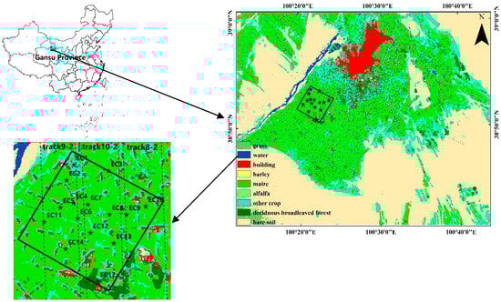
Figure 1.
Geographic location and land cover map of the study area. The land use map was obtained from a monthly land cover map data base of the Heihe River Basin [25]. The map in the lower left contains the approximate locations of the eddy covariance (EC) towers used in the validation of the TSEB fluxes and were deployed within the main experimental domain (rectangular box; EC1 indicated the first EC tower, and so on). The aircraft imagery was collected over portions of the study area, and its spatial coverage is indicated by the dash lines.
2.2. Field Measurements
The surface flux measurements are collected from the Multi-Scale Observation Experiment on Evapotranspiration (MUSOEXE) [26,27], which is the first thematic experiment in the HiWATER. The HiWATER-MUSOEXE established a flux observation network composed of two nested matrices: one large experimental area (30 × 30 km) and one smaller and more intensively instrumented (main) experimental area (5.5 × 5.5 km). The MUSOEXE campaign was conducted in the middle of the Heihe River Basin from May to September 2012. Seventeen EC systems together with automatic weather stations (AWSs) were deployed in the main experimental area. Among the 17 EC systems, 14 were installed in maize fields, and the other three were located in a residential area (EC4 in Figure 1), a vegetable field (EC1 in Figure 1), and an orchard (EC17 in Figure 1), respectively.
The turbulent fluxes were measured by the EC system with a sampling frequency of 10 Hz. The sensor system is described in detail by Wang et al. [28]. Briefly the EC sensors included CSAT3 and EC150 (by Campbell Scientific Inc., Logan, UT, USA), LI-7500/7500A (by LI-COR, USA), and Gill-WM (by Gill Inst. Ltd., U.K.). (The use of trade, firm, or corporation names in this article is for the information and convenience of the reader. Such use does not constitute official endorsement or approval by the US Department of Agriculture or the Agricultural Research Service of any product or service to the exclusion of others that may be suitable.) The raw data were processed using Edire software (http://www.geos.ed.ac.uk/abs/-research/micromet/EdiRE/) and averaged over 30 min. The ground heat flux was measured by using three soil heat flux plates buried at a depth of 5 cm around each EC tower. A soil moisture and temperature measurement system (SMTMS) was installed at each EC site to obtain the soil moisture and temperature profiles [28]. Meteorological data, including air temperature, humidity, wind speed, wind direction, surface pressure, and four components of radiation, were measured by the AWS network. The meteorological, soil moisture, soil temperature, and ground heat flux data were processed to 30 min averages. The soil surface heat flux was derived from the ground heat flux, soil moisture, and soil temperature by combining heat flux plate measurements and calorimetry [29]. Surface temperature was measured by an SI-111 infrared radiometer mounted at a 4 m height above ground on the EC towers. The absolute accuracy of the radiometer is ±0.2 °C. Vegetation structural parameters including leaf area index (LAI), fraction of vegetation cover () and height of the vegetation () were also measured around each EC site during HiWATER-MUSOEXE campaign. LAI was measured 14 times during the growing season using a LiCor (LI-COR, Lincoln, NE, USA) LAI-2000, was estimated using a digital photography method [30], and vegetation height was measured from a transect of ground measurements near the EC tower.
2.3. Aircraft and Satellite Data
The aircraft data were acquired by the Wide-Angle Infrared Dual-Mode Line/Area Array Scanner (WiDAS), which was designed and built by the Institute of Remote Sensing and Digital Earth of the Chinese Academy of Sciences and Beijing Normal University in 2008 [31]. The WiDAS system is comprised of one CCD camera (the wavelength range of five visible and near-infrared (VNIR) channels are 400–500 nm, 500–590 nm, 590–670 nm, 670–850 nm, and 850–1000 nm), one middle-infrared (MIR) camera (3–5 μm), and one thermal-infrared (TIR) camera (7.5–14 μm). The nadir spatial resolutions of the VNIR and TIR channels are 1.2 m and 7.9 m at a 1500 m flight height, respectively. As a wide-angle sensor, the largest view zenith angle is about 30° for the VNIR bands and about 40° for the TIR bands. More details of the WiDAS system is given in [31]. The WiDAS images were acquired in the middle reaches of the Heihe River Basin on 26 July, 2 August, and 3 August 2012. The acquired TIR images were calibrated by a Blackbody Mikron340 and atmospherically corrected using MODTRAN 4.0 with synchronous radio soundings. The VNIR and TIR images were co-registered and resampled to a spatial resolution of 7.5 m. However, comparison to the tower infrared radiometers, there was an observed 4.7 degree bias which was corrected via linear regression. This significantly improved measured-model agreement.
During the HiWATER-MUSOEXE campaign, ASTER images on eight cloud-free days (Day of Year (DOY) 151, 167, 176, 192, 215, 231, 240, and 247) were collected. The data included ASTER standard Level 2 land surface temperature and emissivity products (AST_08 and AST_05) retrieved by the temperature and emissivity separation algorithm [32] and ASTER Level 1 Precision Terrain Corrected Registered At-Sensor Radiance (AST_L1T). The surface reflectance was derived from AST_L1T through correcting the atmospheric effects with the Fast Line-of-sight Atmospheric Analysis of Hypercubes (FLAASH) [33]. The spatial resolution of AST08 is 90 m, and the spatial resolution of visible channels of ASTER is 15 m. Three tracks (Track 8-2, Track 9-2, and Track 10-2) of WiDAS images that cover the main experimental area of the HiWATER-MUSOEXE campaign and ASTER data on 2 August 2012 were used in this study.
3. Methodology
3.1. Model Description
The TSEB model was originally proposed by Norman et al. [10] to partition the energy fluxes between the soil and vegetation through balancing both the radiative temperature and convective (turbulent) heat fluxes of the soil and vegetated canopy components [34]. A number of revisions have been made to accommodate a wider range of land cover and environmental conditions, and to improve the capability of TSEB to partition radiative and convective fluxes between soil and vegetation canopy components under more heterogeneous cover conditions. These include replacing the divergence of net radiation for soil and canopy components with a more physically based algorithm and introducing a clumping factor to the model [35], revising the soil resistance formulation [36], and replacing the Priestley–Taylor with the Penman–Monteith formulation [37], among others. A description of the TSEB model is briefly outlined below. A detailed description of TSEB algorithms has been published multiple times, most recently by Kustas et al. [38] and Nieto et al. [39]. Without considering photosynthesis and advection, the net energy balance of the soil–canopy–atmosphere system is given by
where is the net radiation, is the sensible heat flux, is the latent heat flux absorbed by water vapor when it evaporates from the soil surface and transpires from plants through stomata, and is the soil heat flux. Subscripts “s” and “c” represents the soil and canopy components, respectively. According to Kustas and Norman [35],
where is incident solar radiation, is solar transmittance in the canopy, is soil albedo, and are longwave radiation for soil and canopy, and are estimated via the following expression:
where , , and are longwave radiation from the sky, soil, and canopy, and can be calculated from the Stefan-Boltzmann equation using shelter level air temperature and vapor pressure, soil temperature, and canopy temperature. is a clumping factor to characterize the heterogeneity of surface, and calculated by the formulation of Kustas et al. [36]. is an extinction coefficient, whose calculation can be found in [40], as can the calculation of transmittance, albedo, and extinction coefficients for soil and canopy. The surface soil heat flux is parameterized as a fraction of by
where c is the empirical coefficient and tends to be 0.35, and has been expressed as a function of time to accommodate known temporal variation in this “constant” [41].
Assuming a single emissivity is used to represent the combined soil and vegetation, the ensemble directional radiometric temperature () is determined by the fraction of the radiometer view that is occupied by soil versus vegetation expressed as
where and are vegetation canopy temperature and soil surface temperature. Usually, = 4 for 8–14 μm and 10–12 μm wavelength bands. is the fractional vegetation cover at the thermal sensor view angle . Assuming a spherical leaf angle distribution, is expressed as,
The Priestley-Taylor formula was used to partition the latent heat flux between the soil and vegetation canopy. The latent heat flux from the vegetated canopy () is initially computed as,
where is the Priestley-Taylor parameter, is the fraction of the green LAI, is the slope of the saturation vapor pressure versus temperature curve, and is the psychrometer constant.
After determining the and , and can be solved by combining the energy balance model (Equations (2) and (3)) and Equation (9). When calculating the sensible heat flux , there are two kinds of resistance schemes, “parallel” and ”series”. The former neglects energy exchange between soil and vegetation, while the latter allows such interactions. In this study, the “series” and “parallel” schemes are adopted for the resistance network under unstable and stable conditions, respectively. For more details on model convergence, please refer to Norman et al. [10]. The TSEB has been validated to a great extent over agricultural areas, with variable fractional vegetation cover, and under various climate conditions [42,43,44].
3.2. Generation of Model Inputs
The inputs of TSEB include directional radiometric surface temperature and its viewing angle, clumping index, fractional vegetation cover or leaf area index, vegetation height and approximate leaf width, and meteorological data (i.e., incident solar radiation, air temperature, vapor pressure, surface pressure, and wind speed at a reference height above the surface). The spatial distributions of meteorological parameters are derived by interpolating the measurements collected from the AWS network using the inverse distance weighting method. The land cover map used for ET estimates from WiDAS data was derived from the WiDAS optical data using the object-oriented technique, whereas the land cover map used for the ASTER ET estimate was interpolated from a monthly 30 m land cover map derived from HJ-1/CCD data [25]. The directional radiometric surface temperature was extracted from the AST_08 and WiDAS ground-leaving radiance. The vegetation structure parameters (, and ) were calculated using the established non-linear relationship between the satellite-derived normalized difference vegetation index (NDVI) and field measured vegetation parameters.
We first aggregated the 15 m ASTER NDVI to 90 m to match the spatial resolution of AST_08 TIR data and then established the non-linear relationship at a spatial resolution of 90 m. Previously, the vegetation parameters such as the LAI were estimated using a lookup table method for WiDAS [31]. However, since the WiDAS data were collected under dense vegetation cover conditions with LAI values of the order of 3.5 over much of the study domain, it was not possible to retrieve LAI, fractional cover, and canopy height directly from WiDAS data. Instead, we established non-linear relationships between these plant parameters and the NDVI at a 15 m spatial resolution using ASTER NDVI data and in situ measurements over the growing season. As a result, the vegetation parameters using the WiDAS imagery with TSEB were estimated by interpolating the values from the non-linear NDVI relationships from ASTER at 15 m resolution Figure 2 illustrates the established relationship for , and at 90m spatial resolution. The threshold for bare soil and full vegetation is set to 0.05 and 0.85 when calculating the NDVI. The coefficient of determination for these relationships is between 0.80 and 0.90.
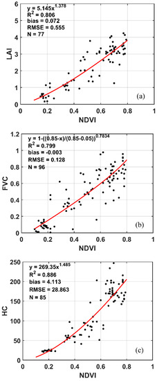
Figure 2.
The established empirical relationship between ASTER NDVI and (a) leaf area index (LAI), (b) fractional canopy cover () and (c) plant canopy height () at 90m spatial resolution.
4. Results and Discussion
4.1. Comparison with EC Measurements
The EC flux measurements typically have an issue of lack of energy closure, namely, the sum of the measured latent and sensible heat fluxes tends to be less than the available energy [45]. The energy imbalance will bring unavoidable bias errors when validating model estimated fluxes. The average closure ratio was computed to be about 80% for the 16 HiWATER EC sites. Usually, we have two methods to enforce the energy closure, the Bowen ratio (BR) method [46] and the residual (RE) approach [47]. According to the studies of Li et al. [34], in well watered maize, the difference in H and LE estimates using the two energy balance closure methods was not significant. However, both energy closure methods were used in this study.
Another issue is the spatial representativeness of the EC system, which can reach hundreds of meters depending on the EC measurement height, wind speed and direction, vegetation height, aerodynamic roughness, and stability. A two-dimensional footprint model is employed to estimate the source area on the land-surface contributing to the eddy flux measurements [48,49], and to provide the prediction model of weighted source-area contribution. The two-dimensional footprint model is expressed as
where is the one-dimensional along-wind footprint model of Hsieh et al. [49], x is the fetch in the upwind direction, is flux observation height, and is the standard deviation in the lateral wind fluctuations. During the comparison between modeled and measured fluxes, we can calculate the gridded model output by integration using the following expression:
where indicates a pixel in the model grid at location (), is the modeled flux in the tower source area.
Figure 3 is a comparison of component fluxes, and the statistical measures are defined in Table 1. The validation data were linearly interpolated from the half hour values surrounding the overpass time of WiDAS or ASTER. Generally, the modeled component fluxes agree reasonably well with those observed, although discrepancies in the modeled and measure G tend to be greater. This may be due in part to the use of only three soil heat flux observations for the sites with more heterogeneous cover conditions, namely the vegetable, orchard, and residential field sites. Hence, the G observations are not adequately sampling the actual spatial and temporal variability in soil heat flux within the tower flux footprint.
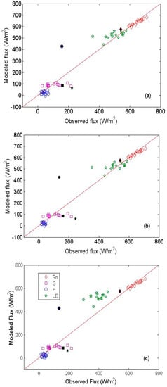
Figure 3.
Comparison between measured and modeled flux components obtained by applying TSEB to WiDAS imagery. Plot (a) is enforcing closure with the BR method; (b) closure with the RE method; and (c) measured H (sensible hear flux) and LE (latent heat flux) without closure. The solid symbols are the modeled and observed flux components for Tower Site 4 (EC4). Rn denotes net radiation, and G denotes soil heat flux.

Table 1.
Statistical performance of the flux components obtained by applying TSEB to WiDAS and ASTER images. The values in parentheses are the statistical results using the ASTER image. The subscripts BR and RE refer to the Bowen ratio and the residual methods enforcing energy balance closure, respectively.
In addition, at Tower Site 4 (EC4), with flux components denoted by solid symbols in Figure 3, which was deployed in a residential area surrounded by buildings, trees, and bordering, an agricultural field is an outlier. Often residential areas will contain trees, lawns, and gardens that border buildings or in open spaces. This causes major difficulties in defining model input parameters for such a complex surface as well as determining the actual source area contributing to the EC flux. Therefore, the relatively large differences between modeled and measured fluxes observed for this complex land cover type is not unexpected.
Whether or not energy balance closure is invoked, the mean absolute percent error (MAPE) is less than 20% for all flux components: Rn, G, H, and LE. The biases for LE closed by the BR and RE approaches are of the order of 15 and 5 W/m2, the RMSE values are 75 and 70 W/m2, and values of MAPEs are 3 and 1%, respectively. Without invoking energy balance closure, the corresponding values of bias for H (LE) are 8 (113) W/m2, RMSE values are 78 (140) W/m2, and MAPE values are 19% (30%). Hence, in general, there is a significant reduction in RMSE and MAPE forcing closure using either the RE or the BR method. Since models conserve energy, it seems reasonable to also enforce energy balance closure with the EC measurements, although errors, principally in soil heat flux measurements, may under certain conditions be significant and hence cause greater uncertainty in tower fluxes. The results with closed fluxes indicate that TSEB performance is satisfactory since the uncertainties of the EC technique is typically of the order of 15–20% for H and LE [20], similar to what was found for the HiWATER-MUSOEXE field campaign [28].
Using ASTER data in TSEB, the agreement with measured H and LE significantly deteriorate, particularly for LE with RMSE values exceeding 130 W/m2. The values become even larger when compared to the unclosed (direct measurement) LE. However, the MAPE values for closed LE of 2 and 4% are still considered acceptable.
4.2. Spatial Pattern of Estimated ET
The spatial pattern of ET estimated from WiDAS and ASTER images are displayed in Figure 4, Figure 5 and Figure 6. Note that the overpass time of each WiDAS track (11:15, 11:41, and 12:06 local time for tracks 8-2, 9-2, and 10-2) and ASTER (12:19 local time) is different, so direct comparisons of the estimated ET of these two sources of land surface temperature were not made. However, it is reasonable to compare the ET patterns and evaluate the spatial distributions produced by TSEB with the ASTER and WIDAS imagery. As seen in both WiDAS and ASTER ET images, as expected, the ET of cropland (vegetation) is higher than the ET of non-cropland land cover types, such as natural semi-arid vegetation land cover containing small fractions of canopy cover, roads, and buildings around midday. Thus, the spatial distribution of high and low ET is likely to reflect the spatial distribution of cropland and non-cropland land covers. With the high resolution WiDAS ET images, we can clearly distinguish the impact of roads that connect residential areas on ET, and the effect on the ET of buildings can also be identified based on this imagery. However, the magnitude and boundaries of reduced ET from roads and buildings is obscured and not readily identified using the ASTER ET images. This result is consistent with the study of Li et al. [48], who found that a pixel resolution of the order of 10 m is much more capable than a ~100 m resolution in discriminating spatial patterns of ET due to land cover, moisture, and vegetation conditions in riparian areas and other landscapes where significant changes in land use occur at over tens of meters.
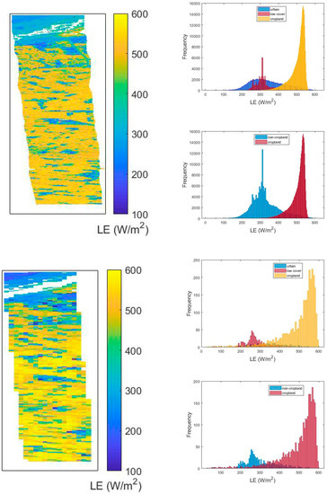
Figure 4.
Comparison between ASTER-derived ET (90 m, lower-left) and ET derived from aircraft image Track 8-2 (7.5 m, upper-left) maps and the associated histograms of the three main land cover types, alternatively combining urban and low canopy cover (semi-arid natural vegetation) under the broad land cover category of non-cropland.
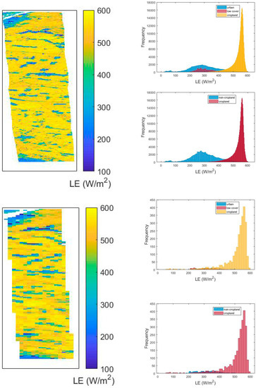
Figure 5.
Comparison between ASTER derived ET (90 m, lower-left) and ET derived from aircraft image Track 9-2 (7.5 m, upper-left) maps and the associated histograms of the three main land cover types, alternatively combining urban and low canopy cover (semi-arid natural vegetation) under the broad land cover category of non-cropland.
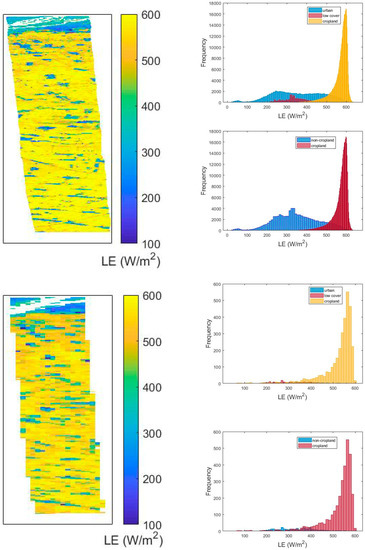
Figure 6.
Comparison between ASTER derived ET (90 m, lower-left) and ET derived from aircraft image Track 10-2 (7.5 m, upper-left) maps and the associated histograms of the three main land cover types, alternatively combining urban and low canopy cover (semi-arid natural vegetation) under the broad land cover category of non-cropland.
4.3. Potential of Monitoring Land Cover Change and Water Use
Land cover change can have a strong effect on the magnitude of ET as well as the hydrological cycle [50,51]. Figure 4, Figure 5 and Figure 6 compare WiDAS and ASTER ET maps as well as the ET histograms of the three land cover types of cropland: urban and low canopy cover (natural semiarid vegetation) and a combination of urban and low canopy cover under non-cropland land cover. Table 2 lists the percentage area estimated for each dominant land cover types and the corresponding mean ET value. As discussed in Section 4.2, the spatial pattern of ET is similar, but high resolution WiDAS ET provides much greater detail regarding the variability in the magnitude of ET and, more accurately, the areal extent and spatial pattern of ET for the different land cover types.
Table 2.
ET values (mean ) and area ratio of each dominant land cover type in the WiDAS and ASTER images. The values in the parentheses represent the values derived from the ASTER image.
The mean ET values of urban and low vegetation cover are similar and are significantly different in magnitude for the cropland, which is irrigated. The ET divergence (standard deviation) of the urban land cover is larger than that of the semi-arid natural vegetation cover and cropland, which is probably due to the fact that there are still mixed pixels even at the WiDAS spatial resolutions. These mixed pixels tend to have greater variability in land surface temperature and cover than that at ASTER pixel resolution, which will tend to dampen these key inputs.
If we combined urban and low cover into the classification of non-cropland, the difference in the mean ET value between non-cropland and cropland is also significant. As shown in Table 2, the mean ET values of non-cropland and cropland are ~nominally 325 and 500 W/m2 for Track 8-2 (Figure 4), 300 and 540 W/m2 for Track 9-2 (Figure 5), and 345 and 570 W/m2 for Track 10-2 (Figure 6). If we look at the ET histogram of non-cropland and cropland, we see an obvious bimodal distribution from WiDAS ET, whereas the bimodal distribution is nearly non-existent using ASTER ET data. Thus, it is possible to distinguish the impact of ET on land cover type from non-cropland and cropland. One of the most common land cover conversions in agricultural areas is a change from cropland to urban/residential due to rapid urbanization. Thus, high resolution WiDAS ET maps (~10 m) can be used to monitoring the often small but rapid land cover change and the resulting shift in water use/ET.
5. Conclusions
ET is a significant component of water and energy cycle at local, regional, and global scales. The physically based TSEB model has been proven to be a powerful tool for predicting surface energy balance and in particular, for ET or water use estimation. In this study, TSEB was first applied to high resolution WiDAS data and ASTER data to estimate ET over an agricultural region and then to evaluate the potential utility of high resolution imagery in creating a more accurate map of ET variation caused by the different land cover types.
The retrieved ET was validated with a network of EC tower measurements. The modeled component fluxes using WiDAS data were in reasonable agreement, with the observed component fluxes with RMSE values in ET closed by the Bowen ratio and residual methods of around 70 W/m2. The only exception was a residential site having a complex mixture of buildings and other impervious material, trees, crops, and other vegetation types within the flux tower footprint. RMSE values in LE were significantly larger at approximately 140 W/m2 without enforcing closure. The errors in ET retrieved from ASTER data were greater, particularly for LE, which had RMSE values larger than 130 W/m2 even with closed fluxes.
Regarding the spatial pattern of ET, the high resolution WiDAS ET distinguished a significant change in LE/ET magnitude and areal extent of the three main land cover types: irrigated cropland, urban (residential/roads/impervious surfaces), and natural semiarid vegetation. The significant changes in LE/ET magnitudes for the different land covers are obscured in the ASTER ET images. By comparison of the ET histograms of urban and low vegetation cover and cropland derived from WiDAS imagery, it is clear that the impact of anthropogenic land cover changes on ET can be monitored with much greater fidelity. This study demonstrates the potential utility of high resolution thermal imagery together with a robust model (TSEB) in detecting deviations in ET due to associated land cover changes in agricultural areas affected by urbanization. In particular, this study provides a potential tool for monitoring the impact on ET due to small perturbations in land cover, most often due to urban expansion or encroachment into agricultural areas.
Author Contributions
W.P.K conceived and designed the study; J.C. performed the study and wrote the paper. All authors participated in the editing of the paper.
Funding
This work was partly supported by the National Key Research and Development Program of China via grant 2016YFA0600101, the National Natural Science Foundation of China via grant 41771365, and the Special Fund for Young Talents of the State Key Laboratory of Remote Sensing Sciences via grant 17ZY-02.
Acknowledgments
We thank all the scientists, engineers, and students who participated in HiWATER field campaigns, Lisheng Song, Yan Li and Ziwei Xu for helping in processing the field measurements. The WiDAS aircraft data and field measurements are downloaded from http://card.westgis.ac.cn/hiwater. USDA is an equal opportunity employer and provider.
Conflicts of Interest
The authors declare no conflict of interest.
References
- Katul, G.G.; Oren, R.; Manzoni, S.; Higgins, C.; Parlange, M.B. Evapotranspiration: A process driving mass transport and energy exchange in the soil-plant-atmosphere-climate system. Rev. Geophys. 2012, 50. [Google Scholar] [CrossRef]
- Kustas, W.P.; Norman, J.M.; Anderson, M.C.; French, A.N. Estimating subpixel surface temperatures and energy fluxes from the vegetation index–radiometric temperature relationship. Remote Sens. Environ. 2003, 85, 429–440. [Google Scholar] [CrossRef]
- Jung, M.; Reichstein, M.; Ciais, P.; Seneviratne, S.I.; Sheffield, J.; Goulden, M.L.; Bonan, G.; Cescatti, A.; Chen, J.Q.; Jeu, R.D. Recent decline in the global land evapotranspiration trend due to limited moisture supply. Nature 2010, 467, 951–954. [Google Scholar] [CrossRef] [PubMed]
- Li, Z.L.; Tang, R.L.; Wan, Z.M.; Bi, Y.Y.; Zhou, C.H.; Tang, B.H.; Yan, G.J.; Zhang, X.Y. A review of current methodologies for regional evapotranspiration estimation from remotely sensed data. Sensors 2009, 9, 3801–3853. [Google Scholar] [CrossRef] [PubMed]
- Gao, G.; Chen, D.L.; Cui, C.Y.; Simelton, E. Trend of estimated actual evapotranspiration over china during 1960–2002. J. Geophys. Res. 2007, 112, D11120. [Google Scholar] [CrossRef]
- Anderson, M.C.; Kustas, W.P.; Norman, J.M.; Hain, C.R.; Mecikalski, J.R.; Schultz, L.; González-Dugo, M.P.; Cammalleri, C.; d’Urso, G.; Pimstein, A.; et al. Mapping daily evapotranspiration at field to continental scales using geostationary and polar orbiting satellite imagery. Hydrol. Earth Syst. Sci. 2011, 15, 223–239. [Google Scholar] [CrossRef]
- Fisher, J.B.; Melton, F.; Middleton, E.; Hain, C.; Anderson, M.; Allen, R.; Mccabe, M.; Hook, S.; Baldocchi, D.; Townsend, P.A. The future of evapotranspiration: Global requirements for ecosystem functioning, carbon and climate feedbacks, agricultural management, and water resources. Water Resour. Res. 2017, 53, 2618–2626. [Google Scholar] [CrossRef]
- Jackson, R.D.; Reginato, R.J.; Idso, S.B. Wheat canopy temperature: A practical tool for evaluating water requirements. Water Resour. Res. 1977, 13, 651–656. [Google Scholar] [CrossRef]
- Wang, K.; Wang, P.; Li, Z.; Cribb, M.; Sparrow, M. A simple method to estimate actual evapotranspiration from a combination of net radiation, vegetation index, and temperature. J. Geophys. Res. Atmos. 2007, 112. [Google Scholar] [CrossRef]
- Norman, J.M.; Kustas, W.P.; Humes, K.S. Source approach for estimating soil and vegetation energy fluxes in observations of directional radiometric surface temperature. Agric. For. Meteorol. 1995, 77, 263–293. [Google Scholar] [CrossRef]
- Kustas, W.; Anderson, M.; Anderson, M.; Twine, T.; Black, A. Advances in thermal infrared remote sensing for land surface modeling. Agric. For. Meteorol. 2009, 149, 2071–2081. [Google Scholar] [CrossRef]
- Bastiaanssen, W.G.M.; Menenti, M.; Feddes, R.A.; Holtslag, A.A.M. The surface energy balance algorithm for land (sebal): Part 1 formulation. J. Hydrol. 1998, 212, 801–811. [Google Scholar]
- Su, Z. The surface energy balance system (sebs) for estimation of turbulent heat fluxes. Hydrol. Earth Syst. Sci. 2002, 6, 85–99. [Google Scholar] [CrossRef]
- Fisher, J.B.; Tu, K.P.; Baldocchi, D.D. Global estimates of the land–atmosphere water flux based on monthly avhrr and islscp-ii data, validated at 16 fluxnet sites. Remote Sens. Environ. 2008, 112, 901–919. [Google Scholar] [CrossRef]
- Yao, Y.; Liang, S.; Cheng, J.; Liu, S.; Fisher, J.B.; Zhang, X.; Jia, K.; Zhao, X.; Qin, Q.; Zhao, B. Modis -driven estimation of terrestrial latent heat flux in china based on a modified priestley–taylor algorithm. Agric. For. Meteorol. 2013, 171–172, 187–202. [Google Scholar] [CrossRef]
- Jiang, L.; Islam, S. Estimation of surface evaporation map over southern great plains using remote sensing data. Water Resour. Res. 2001, 37, 329–340. [Google Scholar] [CrossRef]
- Carlson, T. An overview of the “triangle method” for estimating surface evapotranspiration and soil moisture from satellite imagery. Sensors 2007, 7, 1612–1629. [Google Scholar] [CrossRef]
- Caparrini, F.; Castelli, F.; Entekhabi, D. Estimation of surface turbulent fluxes through assimilation of radiometric surface temperature sequences. J. Hydrometeorol. 2009, 5, 145–159. [Google Scholar] [CrossRef]
- Kustas, W.P.; Anderson, M.C.; Alfieri, J.G.; Knipper, K.; Torres-Rua, A.; Parry, C.K.; Hieto, H.; Agam, N.; White, A.; Gao, F. The grape remote sensing atmospheric profile and evapotranspiration experiment (grapex). Bull. Am. Meteorol. Soc. 2018. [Google Scholar] [CrossRef]
- Kustas, W.P.; Alfieri, J.G.; Anderson, M.C.; Colaizzi, P.D.; Prueger, J.H.; Evett, S.R.; Neale, C.M.U.; French, A.N.; Hipps, L.E.; Chávez, J.L. Evaluating the two-source energy balance model using local thermal and surface flux observations in a strongly advective irrigated agricultural area. Adv. Water Resour. 2012, 50, 120–133. [Google Scholar] [CrossRef]
- Cheng, G.; Li, X.; Zhao, W.; Xu, Z.; Feng, Q.; Xiao, S.; Xiao, H. Integrated study of the water–ecosystem–economy in the heihe river basin. Natl. Sci. Rev. 2014, 1, 413–428. [Google Scholar] [CrossRef]
- Li, X.; Cheng, G.; Liu, S.; Xiao, Q.; Ma, M.; Jin, R.; Che, T.; Liu, Q.; Wang, W.; Qi, Y. Heihe watershed allied telemetry experimental research (hiwater): Scientific objectives and experimental design. Bull. Am. Meteorol. Soc. 2013, 94, 1145–1160. [Google Scholar] [CrossRef]
- Qi, S.-Z.; Luo, F. Water environmental degradation of the heihe river basin in arid northwestern china. Environ. Monit. Assess. 2005, 108, 205–215. [Google Scholar] [CrossRef]
- Chen, Y.; Zhang, D.; Sun, Y.; Liu, X.; Wang, N.; Savenije, H.H.G. Water demand management: A case study of the heihe river basin in China. Phys. Chem. Earth Parts A/B/C 2005, 30, 408–419. [Google Scholar] [CrossRef]
- Zhong, B.; Ma, P.; Nie, A.H.; Yang, A.X.; Yao, Y.J.; Lü, W.B.; Hang, Z.; Liu, Q.H. Land cover mapping using time series hj-1/ccd data. Sci. China Earth Sci. 2014, 57, 1790–1799. [Google Scholar] [CrossRef]
- Liu, S.M.; Xu, Z.W.; Zhu, Z.L.; Jia, Z.Z.; Zhu, M.J. Measurements of evapotranspiration from eddy-covariance systems and large aperture scintillometers in the Hai River Basin, China. J. Hydrol. 2013, 487, 24–38. [Google Scholar] [CrossRef]
- Xu, Z.; Liu, S.; Li, X.; Shi, S.; Wang, J.; Zhu, Z.; Xu, T.; Wang, W.; Ma, M. Intercomparison of surface energy flux measurement systems used during the hiwater-musoexe. J. Geophys. Res. Atmos. 2013, 118, 13–140, 157. [Google Scholar] [CrossRef]
- Wang, J.; Zhuang, J.; Wang, W.; Liu, S.; Xu, Z. Assessment of uncertainties in eddy covariance flux measurement based on intensive flux matrix of hiwater-musoexe. Ieee Geosci. Remote Sens. Lett. 2015, 12, 259–263. [Google Scholar] [CrossRef]
- Liebethal, C.; Huwe, B.; Foken, T. Sensitivity analysis for two ground heat flux calculation approaches. Agric. For. Meteorol. 2005, 132, 253–262. [Google Scholar] [CrossRef]
- Liu, Y.; Mu, X.; Wang, H.; Yan, G. A novel method for extracting green fractional vegetation cover from digital images. J. Veg. Sci. 2012, 23, 406–418. [Google Scholar] [CrossRef]
- Liu, Q.; Yan, C.; Xiao, Q.; Yan, G.; Fang, L. Separating vegetation and soil temperature using airborne multiangular remote sensing image data. Int. J. Appl. Earth Obs. Geoinf. 2012, 17, 66–75. [Google Scholar] [CrossRef]
- Gillespie, A.R.; Rokugawa, S.; Matsunaga, T.; Cothern, J.S.; Hook, S.J.; Kahle, A.B. A temperature and emissivity separation algorithm for advanced spaceborne thermal emission and reflection radiometer (aster) images. IEEE Trans. Geosci. Remote Sens. 1998, 36, 1113–1126. [Google Scholar] [CrossRef]
- Cooley, T.; Anderson, G.P.; Felde, G.W.; Hoke, M.L.; Ratkowski, A.J.; Chetwynd, J.H.; Gardner, J.A.; Adler-Golden, S.M.; Matthew, M.W.; Berk, A. Flaash, a modtran4-based atmospheric correction algorithm, its application and validation. In Proceedings of the 2002 IEEE International Geoscience and Remote Sensing Symposium (IGARSS’02), Westin Harbour Castle, Toronto, ON, Canada, 24–28 June 2002; Volume 1413, pp. 1414–1418. [Google Scholar]
- Li, F.; Kustas, W.P.; Prueger, J.H.; Neale, C.M.U.; Jackson, T.J. Utility of remote sensing based two-source energy balance model under low- and high-vegetation cover conditions. J. Hydrometeorol. 2005, 6, 878–891. [Google Scholar] [CrossRef]
- Kustas, W.P.; Norman, J.M. Evaluation of soil and vegetation heat flux predictions using a simple two-source model with radiometric temperatures for partial canopy cover. Agric. For. Meteorol. 1999, 94, 13–29. [Google Scholar] [CrossRef]
- Kustas, W.P.; Norman, J.M. A two-source energy balance approach using directional radiometric temperature observations for sparse canopy covered surfaces. Agron. J. 2000, 92, 847–854. [Google Scholar] [CrossRef]
- Colaizzi, P.D.; Agam, N.; Tolk, J.A.; Evett, S.R.; Howell, T.A.; Gowda, P.H.; O’Shaughnessy, S.A.; Kustas, W.P.; Anderson, M.C. Two-source energy balance model to calculate e, t, and et: Comparison of priestley-taylor and penman-monteith formulations and two time scaling methods. Trans. Asabe 2014, 57, 479–498. [Google Scholar]
- Kustas, W.P.; Alfieri, J.G.; Nieto, H.; Wilson, T.G.; Gao, F.; Anderson, M.C. Utility of the two-source energy balance (tseb) model in vine and interrow flux partitioning over the growing season. Irrig. Sci. 2018. [Google Scholar] [CrossRef]
- Nieto, H.; Kustas, W.P.; Torres-Rúa, A.; Alfieri, J.G.; Gao, F.; Anderson, M.C.; White, W.A.; Song, L.; Alsina, M.d.M.; Prueger, J.H.; et al. Evaluation of tseb turbulent fluxes using different methods for the retrieval of soil and canopy component temperatures from uav thermal and multispectral imagery. Irrig. Sci. 2018. [Google Scholar] [CrossRef]
- Campbell, G.S.; Norman, J.M. An Introduction to Environmental Biophysics; Springer: New York, NY, USA, 1998. [Google Scholar]
- Santanello, J.A., Jr.; Friedl, M.A. Diurnal covariation in soil heat flux and net radiation. J. Appl. Meteorol. 2003, 42, 851–862. [Google Scholar] [CrossRef]
- Gonzalez-Dugo, M.P.; Neale, C.M.U.; Mateos, L.; Kustas, W.P.; Prueger, J.H.; Anderson, M.C.; Li, F. A comparison of operational remote sensing-based models for estimating crop evapotranspiration. Agric. For. Meteorol. 2009, 149, 1843–1853. [Google Scholar] [CrossRef]
- Timmermans, W.J.; Kustas, W.P.; Anderson, M.C.; French, A.N. An intercomparison of the surface energy balance algorithm for land (sebal) and the two-source energy balance (tseb) modeling schemes. Remote Sens. Environ. 2007, 108, 369–384. [Google Scholar] [CrossRef]
- French, A.N.; Jacob, F.; Anderson, M.C.; Kustas, W.P.; Timmermans, W.; Gieske, A.; Su, Z.; Su, H.; Mccabe, M.F.; Li, F. Surface energy fluxes with the advanced spaceborne thermal emission and reflection radiometer (aster) at the iowa 2002 smacex site (USA). Remote Sens. Environ. 2005, 99, 55–65. [Google Scholar] [CrossRef]
- Massman, W.J.; Lee, X. Eddy covariance flux corrections and uncertainties in long-term studies of carbon and energy exchanges. Agric. For. Meteorol. 2002, 113, 121–144. [Google Scholar] [CrossRef]
- Twine, T.E.; Kustas, W.P.; Norman, J.M.; Cook, D.R.; Houser, P.R.; Meyers, T.P.; Prueger, J.H.; Starks, P.J.; Wesely, M.L. Correcting eddy-covariance flux underestimates over a grassland. Agric. For. Meteorol. 2000, 103, 279–300. [Google Scholar] [CrossRef]
- Falge, E.; Reth, S.; Bruggemann, N.; Butterbach-Bahl, K.; Goldberg, V.; Oltchev, A.; Schaaf, S.; Spindler, G.; Stiller, B.; Queck, R. Comparison of surface energy exchange models with eddy flux data in forest and grassland ecosystems of germany. Ecol. Model. 2005, 188, 174–216. [Google Scholar] [CrossRef]
- Li, F.; Kustas, W.P.; Anderson, M.C.; Prueger, J.H.; Scott, R.L. Effect of remote sensing spatial resolution on interpreting tower-based flux observations. Remote Sens. Environ. 2008, 112, 337–349. [Google Scholar] [CrossRef]
- Hsieh, C.I.; Katul, G.; Chi, T.W. An approximate analytical model for footprint estimation of scalar fluxes in thermally stratified atmospheric flows. Adv. Water Resour. 2000, 23, 765–772. [Google Scholar] [CrossRef]
- Dias, L.C.P.; Macedo, M.N.; Costa, M.H.; Coe, M.T.; Neill, C. Effects of land cover change on evapotranspiration and streamflow of small catchments in the upper xingu river basin, central brazil. J. Hydrol. Reg. Stud. 2015, 4, 108–122. [Google Scholar] [CrossRef]
- Bosmans, J.H.C.; Beek, L.P.H.V.; Sutanudjaja, E.H.; Bierkens, M.F.P. Hydrological impacts of global land cover change and human water use. Hydrol. Earth Syst. Sci. Discuss. 2017, 21, 1–31. [Google Scholar] [CrossRef]
© 2019 by the authors. Licensee MDPI, Basel, Switzerland. This article is an open access article distributed under the terms and conditions of the Creative Commons Attribution (CC BY) license (http://creativecommons.org/licenses/by/4.0/).