A Comparison of Hybrid Machine Learning Algorithms for the Retrieval of Wheat Biophysical Variables from Sentinel-2

 ,
,  , ,
, ,  , and
, and 
Abstract
1. Introduction
2. Materials and Methods
2.1. Generation of PROSAIL Simulations
2.2. Training Machine Learning Algorithms
2.3. Validation with Sentinel-2 Data and Ground Measurements
2.4. Comparative Assessment of MLRAs
3. Results
4. Discussion
5. Conclusions
Author Contributions
Funding
Acknowledgments
Conflicts of Interest
References
- Zhang, C.; Kovacs, J.M. The application of small unmanned aerial systems for precision agriculture: A review. Precis. Agric. 2012, 13, 693–712. [Google Scholar] [CrossRef]
- Jay, S.; Maupas, F.; Bendoula, R.; Gorretta, N. Retrieving LAI, chlorophyll and nitrogen contents in sugar beet crops from multi-angular optical remote sensing: Comparison of vegetation indices and PROSAIL inversion for field phenotyping. Field Crops Res. 2017, 210, 33–46. [Google Scholar] [CrossRef]
- Goffart, J.P.; Olivier, M.; Frankinet, M. Potato crop nitrogen status assessment to improve N fertilization management and efficiency: Past–present–future. Potato Res. 2008, 51, 355–383. [Google Scholar] [CrossRef]
- Cilia, C.; Panigada, C.; Rossini, M.; Meroni, M.; Busetto, L.; Amaducci, S.; Boschetti, M.; Picchi, V.; Colombo, R. Nitrogen status assessment for variable rate fertilization in maize through hyperspectral imagery. Remote Sens. 2014, 6, 6549–6565. [Google Scholar] [CrossRef]
- Verrelst, J.; Rivera, J.P.; Veroustraete, F.; Muñoz-Marí, J.; Clevers, J.G.; Camps-Valls, G.; Moreno, J. Experimental Sentinel-2 LAI estimation using parametric, non-parametric and physical retrieval methods–A comparison. ISPRS J. Photogramm. Remote Sens. 2015, 108, 260–272. [Google Scholar] [CrossRef]
- Jordan, C.F. Derivation of leaf-area index from quality of light on the forest floor. Ecology 1969, 50, 663–666. [Google Scholar] [CrossRef]
- Rouse, J.; Haas, R.; Schell, J.; Deering, D.; Harlan, J. Monitoring the Vernal Advancement of Retrogradation of Natural Vegetation, NASA/GSFC, Type III, Final Report. Available online: https://ntrs.nasa.gov/archive/nasa/casi.ntrs.nasa.gov/19730017588.pdf (accessed on 20 February 2019).
- Rondeaux, G.; Steven, M.; Baret, F. Optimization of soil-adjusted vegetation indices. Remote Sens. Environ. 1996, 55, 95–107. [Google Scholar] [CrossRef]
- Pasolli, E.; Melgani, F.; Alajlan, N.; Bazi, Y. Active learning methods for biophysical parameter estimation. IEEE Trans. Geosci. Remote Sens. 2012, 50, 4071–4084. [Google Scholar] [CrossRef]
- Verrelst, J.; Dethier, S.; Rivera, J.P.; Muñoz-Marí, J.; Camps-Valls, G.; Moreno, J. Active learning methods for efficient hybrid biophysical variable retrieval. IEEE Geosci. Remote Sens. Lett. 2016, 13, 1012–1016. [Google Scholar] [CrossRef]
- Verrelst, J.; Camps-Valls, G.; Muñoz-Marí, J.; Rivera, J.P.; Veroustraete, F.; Clevers, J.G.; Moreno, J. Optical remote sensing and the retrieval of terrestrial vegetation bio-geophysical properties–A review. ISPRS J. Photogramm. Remote Sens. 2015, 108, 273–290. [Google Scholar] [CrossRef]
- Pignatti, S.; Acito, N.; Amato, U.; Casa, R.; Castaldi, F.; Coluzzi, R.; De Bonis, R.; Diani, M.; Imbrenda, V.; Laneve, G.; et al. Environmental products overview of the Italian hyperspectral prisma mission: The SAP4PRISMA project. In Proceedings of the 2015 IEEE International Geoscience and Remote Sensing Symposium (IGARSS), Milan, Italy, 26–31 July 2015. [Google Scholar]
- Guanter, L.; Kaufmann, H.; Segl, K.; Foerster, S.; Rogass, C.; Chabrillat, S.; Kuester, T.; Hollstein, A.; Rossner, G.; Chlebek, C. The EnMAP spaceborne imaging spectroscopy mission for earth observation. Remote Sens. 2015, 7, 8830–8857. [Google Scholar] [CrossRef]
- Durbha, S.S.; King, R.L.; Younan, N.H. Support vector machines regression for retrieval of leaf area index from multiangle imaging spectroradiometer. Remote Sens. Environ. 2007, 107, 348–361. [Google Scholar] [CrossRef]
- Lázaro-Gredilla, M.; Titsias, M.K.; Verrelst, J.; Camps-Valls, G. Retrieval of biophysical parameters with heteroscedastic Gaussian processes. IEEE Geosci. Remote Sens. Lett. 2014, 11, 838–842. [Google Scholar] [CrossRef]
- Verrelst, J.; Malenovský, Z.; Van der Tol, C.; Camps-Valls, G.; Gastellu-Etchegorry, J.-P.; Lewis, P.; North, P.; Moreno, J. Quantifying Vegetation Biophysical Variables from Imaging Spectroscopy Data: A Review on Retrieval Methods. Surv. Geophys. 2018, 1–41. (in press). [CrossRef]
- Knudby, A.; LeDrew, E.; Brenning, A. Predictive mapping of reef fish species richness, diversity and biomass in Zanzibar using IKONOS imagery and machine-learning techniques. Remote Sens. Environ. 2010, 114, 1230–1241. [Google Scholar] [CrossRef]
- Verrelst, J.; Muñoz, J.; Alonso, L.; Delegido, J.; Rivera, J.P.; Camps-Valls, G.; Moreno, J. Machine learning regression algorithms for biophysical parameter retrieval: Opportunities for Sentinel-2 and-3. Remote Sens. Environ. 2012, 118, 127–139. [Google Scholar] [CrossRef]
- Wang, L.; Zhou, X.; Zhu, X.; Dong, Z.; Guo, W. Estimation of biomass in wheat using random forest regression algorithm and remote sensing data. Crop J. 2016, 4, 212–219. [Google Scholar] [CrossRef]
- Benítez, J.M.; Castro, J.L.; Requena, I. Are artificial neural networks black boxes? IEEE Trans. Neural Netw. 1997, 8, 1156–1164. [Google Scholar] [CrossRef] [PubMed]
- Rivera, J.P.; Verrelst, J.; Leonenko, G.; Moreno, J. Multiple cost functions and regularization options for improved retrieval of leaf chlorophyll content and LAI through inversion of the PROSAIL model. Remote Sens. 2013, 5, 3280–3304. [Google Scholar] [CrossRef]
- Combal, B.; Baret, F.; Weiss, M.; Trubuil, A.; Mace, D.; Pragnere, A.; Myneni, R.; Knyazikhin, Y.; Wang, L. Retrieval of canopy biophysical variables from bidirectional reflectance: Using prior information to solve the ill-posed inverse problem. Remote Sens. Environ. 2003, 84, 1–15. [Google Scholar] [CrossRef]
- Atzberger, C. Object-based retrieval of biophysical canopy variables using artificial neural nets and radiative transfer models. Remote Sens. Environ. 2004, 93, 53–67. [Google Scholar] [CrossRef]
- Houborg, R.; Boegh, E. Mapping leaf chlorophyll and leaf area index using inverse and forward canopy reflectance modeling and SPOT reflectance data. Remote Sens. Environ. 2008, 112, 186–202. [Google Scholar] [CrossRef]
- Pozdnyakov, D.; Shuchman, R.; Korosov, A.; Hatt, C. Operational algorithm for the retrieval of water quality in the Great Lakes. Remote Sens. Environ. 2005, 97, 352–370. [Google Scholar] [CrossRef]
- Schiller, H.; Doerffer, R. Improved determination of coastal water constituent concentrations from MERIS data. IEEE Trans. Geosci. Remote Sens. 2005, 43, 1585–1591. [Google Scholar] [CrossRef]
- Verger, A.; Baret, F.; Weiss, M. Performances of neural networks for deriving LAI estimates from existing CYCLOPES and MODIS products. Remote Sens. Environ. 2008, 112, 2789–2803. [Google Scholar] [CrossRef]
- Verger, A.; Baret, F.; Camacho, F. Optimal modalities for radiative transfer-neural network estimation of canopy biophysical characteristics: Evaluation over an agricultural area with CHRIS/PROBA observations. Remote Sens. Environ. 2011, 115, 415–426. [Google Scholar] [CrossRef]
- Weiss, M.; Baret, F. S2ToolBox Level 2 Products: LAI, FAPAR, FCOVER. Available online: https://step.esa.int/docs/extra/ATBD_S2ToolBox_L2B_V1.1.pdf (accessed on 21 February 2019).
- Chai, L.; Qu, Y.; Zhang, L.; Wang, J. Lai retrieval from cyclopes and modis products using artificial neural networks. In Proceedings of the 2008 Geoscience and Remote Sensing Symposium, Boston, MA, USA, 7–11 July 2008. [Google Scholar]
- Camps-Valls, G.; Bruzzone, L. Kernel Methods for Remote Sensing Data Analysis; John Wiley & Sons: Hoboken, NJ, USA, 2009. [Google Scholar]
- Verrelst, J.; Alonso, L.; Caicedo, J.P.R.; Moreno, J.; Camps-Valls, G. Gaussian process retrieval of chlorophyll content from imaging spectroscopy data. IEEE J. Sel. Top. Appl. Earth Obs. Remote Sens. 2013, 6, 867–874. [Google Scholar] [CrossRef]
- Verrelst, J.; Rivera, J.P.; Moreno, J.; Camps-Valls, G. Gaussian processes uncertainty estimates in experimental Sentinel-2 LAI and leaf chlorophyll content retrieval. ISPRS J. Photogramm. Remote Sens. 2013, 86, 157–167. [Google Scholar] [CrossRef]
- Verrelst, J.; Rivera, J.P.; Gitelson, A.; Delegido, J.; Moreno, J.; Camps-Valls, G. Spectral band selection for vegetation properties retrieval using Gaussian processes regression. Int. J. Appl. Earth Obs. Geoinf. 2016, 52, 554–567. [Google Scholar] [CrossRef]
- Settles, B. Active Learning Literature Survey. Available online: http://burrsettles.com/pub/settles.activelearning.pdf (accessed on 21 January 2019).
- Gascon, F.; Bouzinac, C.; Thépaut, O.; Jung, M.; Francesconi, B.; Louis, J.; Lonjou, V.; Lafrance, B.; Massera, S.; Gaudel-Vacaresse, A. Copernicus Sentinel-2A calibration and products validation status. Remote Sens. 2017, 9, 584. [Google Scholar] [CrossRef]
- Jacquemoud, S.; Verhoef, W.; Baret, F.; Bacour, C.; Zarco-Tejada, P.J.; Asner, G.P.; François, C.; Ustin, S.L. PROSPECT+ SAIL models: A review of use for vegetation characterization. Remote Sens. Environ. 2009, 113, S56–S66. [Google Scholar] [CrossRef]
- Feret, J.-B.; François, C.; Asner, G.P.; Gitelson, A.A.; Martin, R.E.; Bidel, L.P.; Ustin, S.L.; Le Maire, G.; Jacquemoud, S. PROSPECT-4 and 5: Advances in the leaf optical properties model separating photosynthetic pigments. Remote Sens. Environ. 2008, 112, 3030–3043. [Google Scholar] [CrossRef]
- Verhoef, W. Light scattering by leaf layers with application to canopy reflectance modeling: The SAIL model. Remote Sens. Environ. 1984, 16, 125–141. [Google Scholar] [CrossRef]
- Meroni, M.; Colombo, R.; Panigada, C. Inversion of a radiative transfer model with hyperspectral observations for LAI mapping in poplar plantations. Remote Sens. Environ. 2004, 92, 195–206. [Google Scholar] [CrossRef]
- Richter, K.; Atzberger, C.; Vuolo, F.; Weihs, P.; d’Urso, G. Experimental assessment of the Sentinel-2 band setting for RTM-based LAI retrieval of sugar beet and maize. Can. J. Remote Sens. 2009, 35, 230–247. [Google Scholar] [CrossRef]
- Richter, R.; Schlapfer, D.; Muller, A. Operational atmospheric correction for imaging spectrometers accounting for the smile effect. IEEE Trans. Geosci. Remote Sens. 2011, 49, 1772–1780. [Google Scholar] [CrossRef]
- Palacharla, P.K.; Durbha, S.S.; King, R.L.; Gokaraju, B.; Lawrence, G.W. A hyperspectral reflectance data based model inversion methodology to detect reniform nematodes in cotton. In Proceedings of the 6th International Workshop on the Analysis of Multi-Temporal Remote Sensing Images (Multi-Temp), Trento, Italy, 12–14 July 2011. [Google Scholar]
- Le Maire, G.; Marsden, C.; Verhoef, W.; Ponzoni, F.J.; Seen, D.L.; Bégué, A.; Stape, J.-L.; Nouvellon, Y. Leaf area index estimation with MODIS reflectance time series and model inversion during full rotations of Eucalyptus plantations. Remote Sens. Environ. 2011, 115, 586–599. [Google Scholar] [CrossRef]
- Si, Y.; Schlerf, M.; Zurita-Milla, R.; Skidmore, A.; Wang, T. Mapping spatio-temporal variation of grassland quantity and quality using MERIS data and the PROSAIL model. Remote Sens. Environ. 2012, 121, 415–425. [Google Scholar]
- Liang, L.; Qin, Z.; Zhao, S.; Di, L.; Zhang, C.; Deng, M.; Lin, H.; Zhang, L.; Wang, L.; Liu, Z. Estimating crop chlorophyll content with hyperspectral vegetation indices and the hybrid inversion method. Int. J. Remote Sens. 2016, 37, 2923–2949. [Google Scholar] [CrossRef]
- Bacour, C.; Jacquemoud, S.; Tourbier, Y.; Dechambre, M.; Frangi, J.-P. Design and analysis of numerical experiments to compare four canopy reflectance models. Remote Sens. Environ. 2002, 79, 72–83. [Google Scholar] [CrossRef]
- Baret, F.; Hagolle, O.; Geiger, B.; Bicheron, P.; Miras, B.; Huc, M.; Berthelot, B.; Niño, F.; Weiss, M.; Samain, O.; et al. LAI, fAPAR and fCover CYCLOPES global products derived from VEGETATION. Remote Sens. Environ. 2007, 110, 275–286. [Google Scholar] [CrossRef]
- Bajwa, S.G.; Gowda, P.H.; Howell, T.A.; Leh, M. Comparing Artificial Neural Network and Least Square Regression Techniques for LAI Retrieval from Remote Sensing Data. Available online: http://www.asprs.org/a/publications/proceedings/pecora17/0006.pdf (accessed on 21 February 2019).
- Geladi, P.; Kowalski, B.R. Partial least-squares regression: A tutorial. Anal. Chim. Acta 1986, 185, 1–17. [Google Scholar] [CrossRef]
- Hagan, M.T.; Menhaj, M.B. Training feedforward networks with the Marquardt algorithm. IEEE Trans. Neural Netw. 1994, 5, 989–993. [Google Scholar] [CrossRef] [PubMed]
- Breiman, L.; Friedman, J.H.; Olshen, R.A.; Stone, C.J. Classification and Regression Trees; Routledge: New York, NY, USA, 1984. [Google Scholar]
- Friedman, J.; Hastie, T.; Tibshirani, R. Additive logistic regression: A statistical view of boosting (with discussion and a rejoinder by the authors). Ann. Stat. 2000, 28, 337–407. [Google Scholar] [CrossRef]
- Breiman, L. Bagging predictors. Mach. Learn. 1996, 24, 123–140. [Google Scholar] [CrossRef]
- Breiman, L. Random forests. Mach. Learn. 2001, 45, 5–32. [Google Scholar] [CrossRef]
- Williams, C.K.; Rasmussen, C.E. Gaussian Processes for Machine Learning. Available online: http://www.gaussianprocess.org/gpml/chapters/RW.pdf (accessed on 20 February 2019).
- Williams, C.K.; Rasmussen, C.E. Gaussian Processes for Regression. Available online: https://pdfs.semanticscholar.org/e251/664b68fe1b2bdbf39d938b96adfabe54c4fd.pdf (accessed on 20 February 2019).
- Verrelst, J.; Rivera, J.; Alonso, L.; Moreno, J. ARTMO: An Automated Radiative Transfer Models Operator Toolbox for Automated Retrieval of Biophysical Parameters Through Model Inversion. Available online: http://ipl.uv.es/artmo/files/JV_ARTMO_paper_Earsel.pdf (accessed on 20 February 2019).
- Camacho, F.; Baret, F.; Weiss, M.; Fernandes, R.; Berthelot, B.; Sánchez, J.; Latorre, C.; García-Haro, J.; Duca, R. Validación de algoritmos para la obtención de variables biofísicas con datos Sentinel2 en la ESA: Proyecto VALSE-2. In Proceedings of the XV Congreso de la Asociación Española de Teledetección INTA, Torrejón de Ardoz (Madrid), 22–24 October 2013. [Google Scholar] [CrossRef]
- Li-Cor, I. LAI-2000 Plant Canopy Analyzer Instruction Manual; LI-COR Inc.: Lincoln, NE, USA, 1992. [Google Scholar]
- Casa, R.; Castaldi, F.; Pascucci, S.; Pignatti, S. Chlorophyll estimation in field crops: An assessment of handheld leaf meters and spectral reflectance measurements. J. Agric. Sci. 2015, 153, 876–890. [Google Scholar] [CrossRef]
- Nielsen, D.C.; Miceli-Garcia, J.J.; Lyon, D.J. Canopy cover and leaf area index relationships for wheat, triticale, and corn. Agron. J. 2012, 104, 1569–1573. [Google Scholar] [CrossRef]
- Das, B.; Nair, B.; Reddy, V.K.; Venkatesh, P. Evaluation of multiple linear, neural network and penalised regression models for prediction of rice yield based on weather parameters for west coast of India. Int. J. Biometeorol. 2018, 62, 1809–1822. [Google Scholar] [CrossRef] [PubMed]
- Clevers, J.G.; Kooistra, L.; van den Brande, M.M. Using Sentinel-2 data for retrieving LAI and leaf and canopy chlorophyll content of a potato crop. Remote Sens. 2017, 9, 405. [Google Scholar] [CrossRef]
- Frampton, W.J.; Dash, J.; Watmough, G.; Milton, E.J. Evaluating the capabilities of Sentinel-2 for quantitative estimation of biophysical variables in vegetation. ISPRS J. Photogramm. Remote Sens. 2013, 82, 83–92. [Google Scholar] [CrossRef]
- Drusch, M.; Gascon, F.; Berger, M. GMES Sentinel-2 Mission Requirements Document. Available online: https://earth.esa.int/pub/ESA_DOC/GMES_Sentinel2_MRD_issue_2.0_update.pdf (accessed on 20 February 2019).


| Variable | Units | Min | Max | Mode | SD | Class | Law | |
|---|---|---|---|---|---|---|---|---|
| Canopy | Leaf area index (LAI) | - | 0 | 15 | 2 | 2 | 6 | log_normal |
| Avearge leaf angle (ALA) | - | 30 | 80 | 60 | 20 | 3 | gaussian | |
| Hot spot parameter (HsD) | - | 0.1 | 0.5 | 0.2 | 0.5 | 1 | gaussian | |
| Leaf structure index (N) | - | 1.2 | 1.8 | 1.5 | 0.3 | 3 | gaussian | |
| Leaf | Leaf chlorophyll content (LCC) | µg cm−2 | 20 | 90 | 45 | 30 | 4 | gaussian |
| Leaf dry matter content (Cdm) | g cm−2 | 0.003 | 0.011 | 0.005 | 0.005 | 4 | gaussian | |
| Leaf water content (Cw_Rel) | - | 0.6 | 0.85 | 0.75 | 0.08 | 4 | uniform | |
| Brown pigments (Cbp) | - | 0 | 2 | 0 | 0.3 | 3 | gaussian | |
| Soil | Soil brightness (Bs) | - | 0.5 | 3.5 | 1.2 | 2 | 4 | gaussian |
| Algorithm | Brief Description | References |
|---|---|---|
| LSLR | Least Square Linear Regression relies on the linear relationship between explanatory variables, parameters, and the output variable. | [49] |
| PLSR | Partial Least Square Regression performs the regression on the projections generated using partial least squares approach. | [50] |
| NN | Neural Networks is an architecture composed of multiple layers of artificial neurons. For this study, hyperbolic tangent function was used and NN architecture was optimized with the Levenberg–Marquardt learning algorithm with a loss function. | [5,18,51] |
| RegT | Regression Trees was initially a classical approach of decision trees, in which sorting and grouping methods were added to model non-linear relationships. | [52] |
| BooT | Boosting Trees works by sequentially applying a classification algorithm to reweighted versions of the training data and then taking a weighted majority vote of the sequence of the classifiers thus produced. | [5,53] |
| BagT | Bagging Trees is a method for generating multiple versions of a predictor and using them to obtain an aggregated predictor. | [54] |
| RFFE | Random Forest Fit Ensemble is an ensemble to decision tree-based approach for improving the prediction accuracy, such that each tree depends on the values of a random vector sampled independently and with the same distribution for all trees in the forest. | [55] |
| RFTB | Random Forest Tree Bagger combines the bagging approach with the generalized approach of random forest of aggregating multiple decision trees. | [54,55] |
| GPR | Gaussian Process Regression are non-parametric kernel-based probabilistic models, based on Gaussian processes. They are described as a collection of random variables, any finite number of which have a joint Gaussian distribution. GPR also provides uncertainty estimates with the mean value of prediction. | [56,57] |
| Site | Date-Ground Measurements | Date-S2 Acquisition | Difference (Days) |
|---|---|---|---|
| Maccarese, Italy | 31 January 2018 | 29 January 2018 | 2 |
| 16 February 2018 | 13 February 2018 | 3 | |
| 6 April 2018 | 6 April 2018 | 0 | |
| 20 April 2018 | 19 April 18 | 1 | |
| Shunyi, China | 7–8 April 2016 | 10 April 2016 | 2 |
| 20–21 April 2016 | 23 April 2016 | 2 | |
| 3–5 May 2016 | 3 May 2016 | 0 | |
| 18–19 May 2016 | 14 May 2016 | 4 |
| MLRA | LAI | LCC | CCC | FVC | FAPAR | |||||
|---|---|---|---|---|---|---|---|---|---|---|
| CV | GV | CV | GV | CV | GV | CV | GV | CV | GV | |
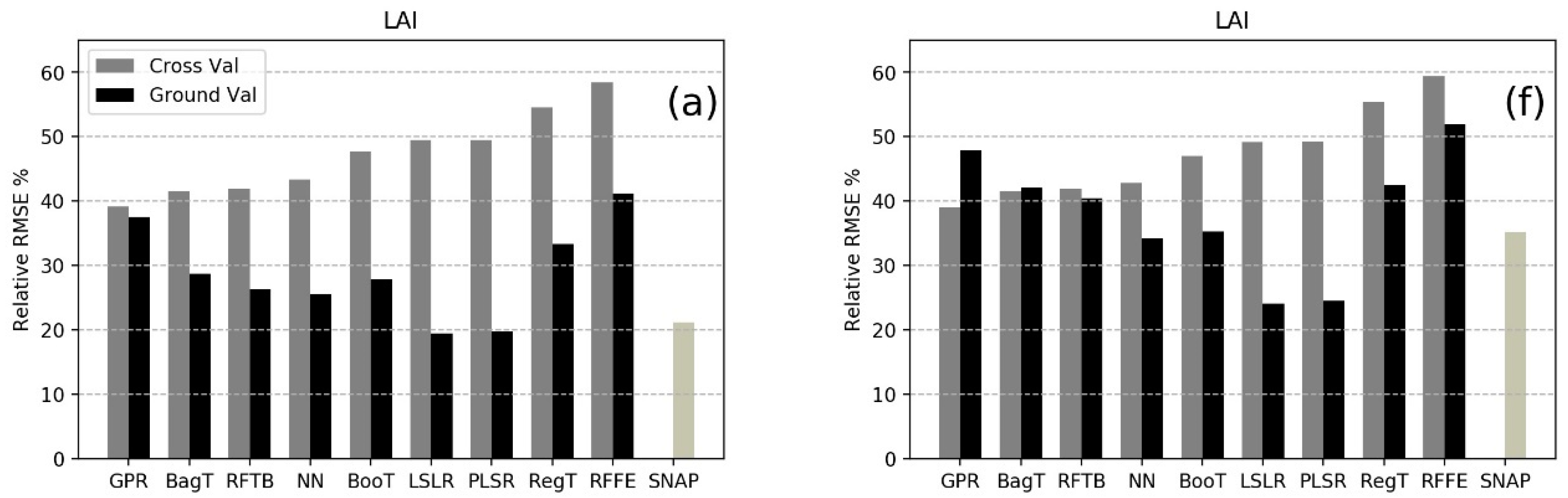
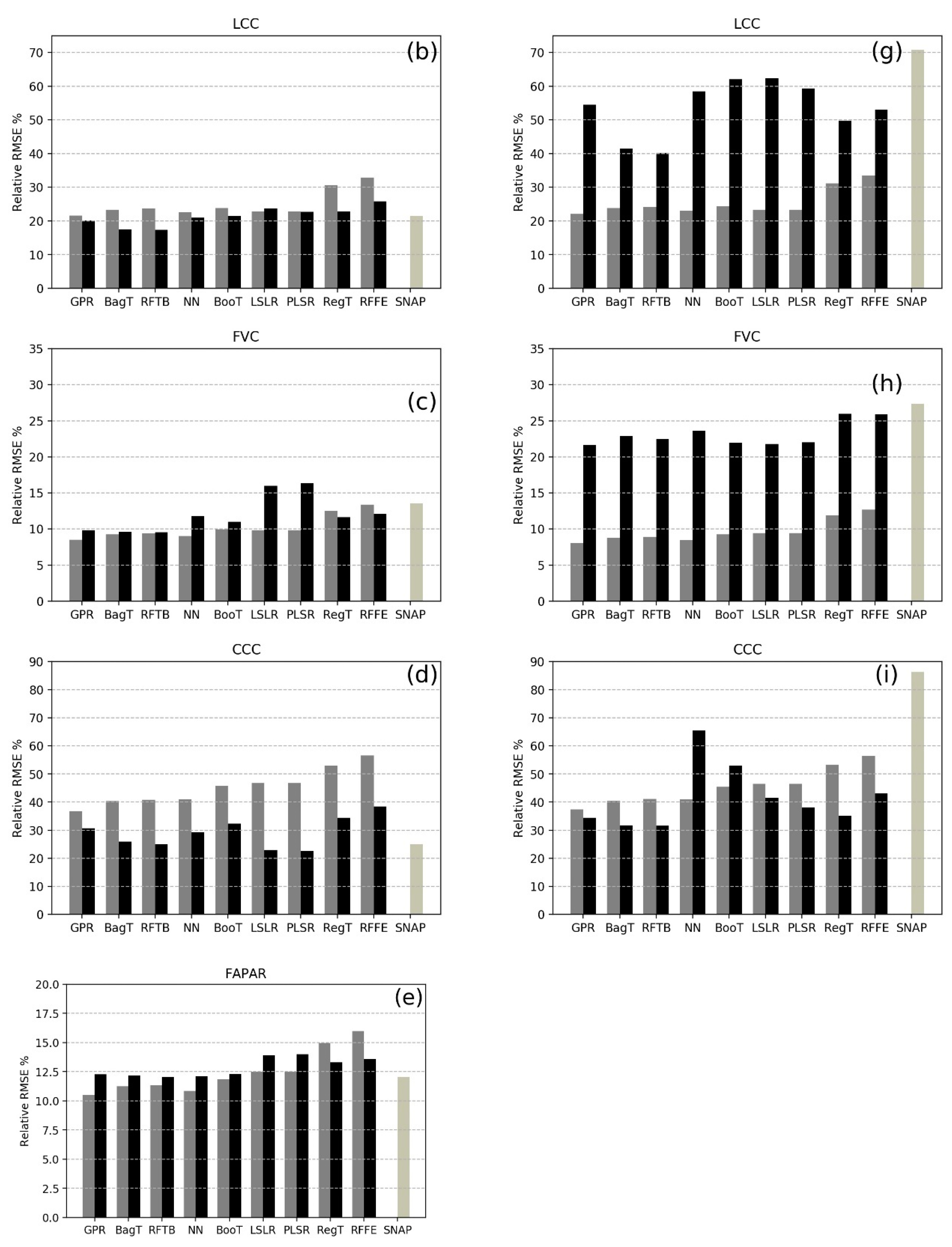
| BagT | 0.99 b | 1.01 d | 11.4 c | 8.90 a | 45.83 a,b | 46.12 b | 0.05 c | 0.08 a | 0.08 c | 0.11 a |
| NN (ARTMO) | 1.04 c | 0.90 b | 11.02 b | 10.68 b,c | 46.53 b | 52.1 c | 0.05 b | 0.09 b,c | 0.07 b | 0.11 a |
| RFTB | 1.00 b | 0.93b c | 11.55 c,d | 8.88 a | 46.47 b | 44.71 b | 0.06 d | 0.08 a | 0.08 c | 0.10 a |
| PLSR | 1.18 e | 0.69 a | 11.16 b | 11.6 c,d | 53.25 c | 40.44 a | 0.06 e | 0.13 d | 0.09 e | 0.12 b |
| LSLR | 1.18 e | 0.68 a | 11.15 b | 12.05 d | 53.14 c | 40.86 a | 0.06 e | 0.13 d | 0.09 e | 0.12 b |
| BooT | 1.14 d | 0.98 c,d | 11.61 d | 10.94 b,c | 52.08 c | 57.51 c,d | 0.06 f | 0.09 b | 0.08 d | 0.11 a |
| RegT | 1.30 f | 1.17 e | 14.99 e | 11.63 c,d | 60.26 d | 61.22 d,e | 0.07 g | 0.09 b,c | 0.10 f | 0.12 b |
| RFFE | 1.40 g | 1.44 f | 16.03 f | 13.18 d | 64.36 d | 68.32 e | 0.08 h | 0.10 c | 0.11 g | 0.12 b |
| GPR + AL | 0.94 a | 1.31 f | 10.55 a | 10.22 b | 43.81 a | 54.56 c | 0.05 a | 0.08 a | 0.07 a | 0.11 a |
| NN (SNAP) | 0.74 | 10.94 | 44.61 | 0.108 | 0.105 | |||||
| MLRA | LAI | LCC | CCC | FVC | ||||
|---|---|---|---|---|---|---|---|---|
| CV | GV | CV | GV | CV | GV | CV | GV | |
| BagT | 0.99 b | 1.74 c,d | 11.67 d | 17.28 a | 46.12 b | 56.72 a | 0.05 c | 0.19 c |
| NN(ARTMO) | 1.02 b | 1.42 b | 11.27 b | 24.41 c | 46.52 b | 98.14 e | 0.05 b | 0.17 a |
| RFTB | 1.00 b | 1.67 c | 11.8 e | 16.77 a | 46.69 b | 56.51 a | 0.05 d | 0.19 c |
| PLSR | 1.18 d | 1.01 a | 11.43 c | 24.77 c | 52.94 c | 68.11 c | 0.06 f | 0.18 b |
| LSLR | 1.18 d | 1.00 a | 11.43 b,c | 25.98 b,c | 52.86 c | 74.33 d | 0.06 f | 0.18 b |
| BooT | 1.12 c | 1.46 b | 11.91 e | 25.91 d | 51.69 c | 94.77 e | 0.05 e | 0.18 b |
| RegT | 1.32 e | 1.76 d | 15.26 f | 20.75 b | 60.63 d | 62.71 b | 0.07 g | 0.21 d |
| RFFE | 1.42 e | 2.14 e | 16.36 g | 25.62 b | 64.29 d | 76.96 d | 0.07 h | 0.21 d |
| GPR + AL | 0.93 a | 1.98 e | 10.79 a | 22.75 b | 42.55 a | 61.35 b | 0.05 a | 0.18 b |
| NN (SNAP) | 1.16 | 23.61 | 123.53 | 0.18 | ||||
| MLRA | 29 January 2018 | 13 February 2018 | 6 April 2018 | 20 April 2018 | ||||
|---|---|---|---|---|---|---|---|---|
| R2 | RMSE | R2 | RMSE | R2 | RMSE | R2 | RMSE | |
| LSLR (LAI) | 0.89 | 0.59 | 0.88 | 0.55 | 0.73 | 0.51 | 0.55 | 1.09 |
| RFTB (LCC) | 0.91 | 3.01 | 0.55 | 7.75 | 0.25 | 12.56 | 0.11 | 7.03 |
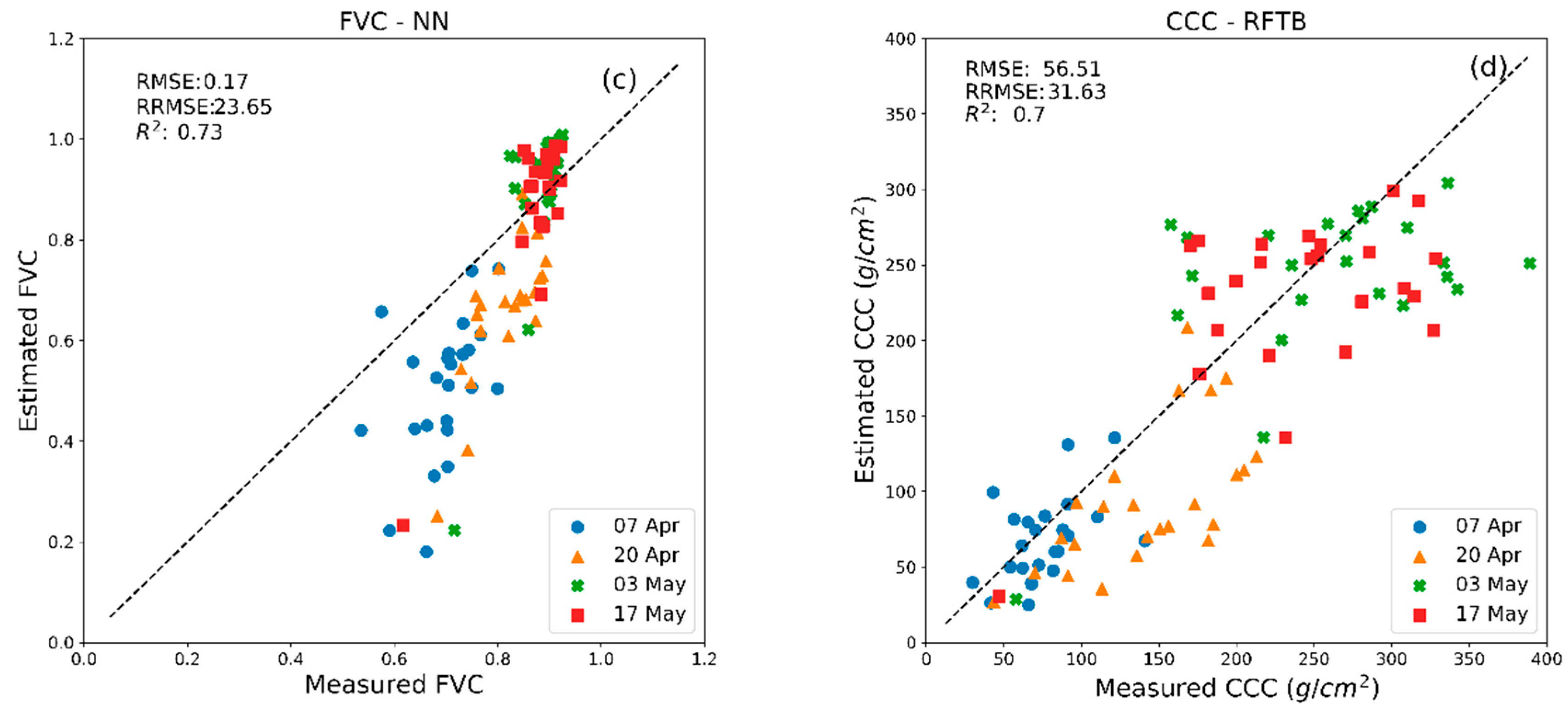
| GPR (FVC) | 0.90 | 0.12 | 0.89 | 0.08 | 0.90 | 0.05 | 0.71 | 0.05 |
| RFTB (FAPAR) | 0.74 | 0.10 | 0.45 | 0.14 | 0.44 | 0.09 | 0.56 | 0.06 |
| PLSR (CCC) | 0.94 | 26.32 | 0.87 | 33.37 | 0.65 | 44.46 | 0.45 | 55.97 |
© 2019 by the authors. Licensee MDPI, Basel, Switzerland. This article is an open access article distributed under the terms and conditions of the Creative Commons Attribution (CC BY) license (http://creativecommons.org/licenses/by/4.0/).
Share and Cite
Upreti, D.; Huang, W.; Kong, W.; Pascucci, S.; Pignatti, S.; Zhou, X.; Ye, H.; Casa, R. A Comparison of Hybrid Machine Learning Algorithms for the Retrieval of Wheat Biophysical Variables from Sentinel-2. Remote Sens. 2019, 11, 481. https://doi.org/10.3390/rs11050481
Upreti D, Huang W, Kong W, Pascucci S, Pignatti S, Zhou X, Ye H, Casa R. A Comparison of Hybrid Machine Learning Algorithms for the Retrieval of Wheat Biophysical Variables from Sentinel-2. Remote Sensing. 2019; 11(5):481. https://doi.org/10.3390/rs11050481
Chicago/Turabian StyleUpreti, Deepak, Wenjiang Huang, Weiping Kong, Simone Pascucci, Stefano Pignatti, Xianfeng Zhou, Huichun Ye, and Raffaele Casa. 2019. "A Comparison of Hybrid Machine Learning Algorithms for the Retrieval of Wheat Biophysical Variables from Sentinel-2" Remote Sensing 11, no. 5: 481. https://doi.org/10.3390/rs11050481
APA StyleUpreti, D., Huang, W., Kong, W., Pascucci, S., Pignatti, S., Zhou, X., Ye, H., & Casa, R. (2019). A Comparison of Hybrid Machine Learning Algorithms for the Retrieval of Wheat Biophysical Variables from Sentinel-2. Remote Sensing, 11(5), 481. https://doi.org/10.3390/rs11050481