A Multi-Scale Filtering Building Index for Building Extraction in Very High-Resolution Satellite Imagery

Abstract

Building extraction plays a significant role in many high-resolution remote sensing image applications. Many current building extraction methods need training samples while it is common knowledge that different samples often lead to different generalization ability. Morphological building index (MBI), representing morphological features of building regions in an index form, can effectively extract building regions especially in Chinese urban regions without any training samples and has drawn much attention. However, some problems like the heavy computation cost of multi-scale and multi-direction morphological operations still exist. In this paper, a multi-scale filtering building index (MFBI) is proposed in the hope of overcoming these drawbacks and dealing with the increasing noise in very high-resolution remote sensing image. The profile of multi-scale average filtering is averaged and normalized to generate this index. Moreover, to fully utilize the relatively little spectral information in very high-resolution remote sensing image, two scenarios to generate the multi-channel multi-scale filtering index (MMFBI) are proposed. While no high-resolution remote sensing image building extraction dataset is open to the public now and the current very high-resolution remote sensing image building extraction datasets usually contain samples from the Northern American or European regions, we offer a very high-resolution remote sensing image building extraction datasets in which the samples contain multiple building styles from multiple Chinese regions. The proposed MFBI and MMFBI outperform MBI and the currently used object based segmentation method on the dataset, with a high recall and F-score. Meanwhile, the computation time of MFBI and MBI is compared on three large-scale very high-resolution satellite image and the sensitivity analysis demonstrates the robustness of the proposed method.

1. Introduction

Building extraction plays a significant role in a series of high-resolution remote sensing applications (e.g., urban extension monitoring, urban mapping and planning, spatial analysis) [1,2,3,4]. Especially in China, for the last thirty to forty years, rapid urbanization has been witnessed, resulting in the eager need of these remote sensing applications [5,6,7,8].

In the 20th century, with only middle and coarse spatial resolution remotely sensed imagery, built-up area extraction is usually a secondary product of land use and land cover classification [9,10,11]. Subject to the spatial resolution at that time, some applications mentioned above like illegal building detection and geo-database updating were unable to implement. It has been reported that only with a spatial resolution of less than five meters, can the single building be clearly represented in imagery [12,13].

For the last twenty to thirty years, the spatial resolution has been improved significantly. For example, the well-known Quick Bird image has a spatial resolution of 0.6 m, and the newly launched WorldView-3 image has a spatial resolution of 0.3 m. The largely increased spatial resolution makes some applications like object detection, geo-database updating and illegal building detection become possible [14,15,16,17,18,19,20,21]. Usually, remotely sensed imagery with a spatial resolution of about 4 to 1 m is called high-resolution remotely sensed imagery (HRRSI) and remotely sensed imagery with a spatial resolution of less than 1 meter is called very high-resolution remotely sensed imagery (VHRRSI) [22,23,24,25].

At the beginning of the 21st century, many studies focused on building extraction with HRRSI. Mathematical morphology, a theory that has been widely used in remote sensing image processing, provides a theoretical fundament for many methods like morphological profiles (MP) [26], differential morphological profiles (DMP) [27], extended morphological profiles (EMP) [28] and attribute profiles (AP) [29]. The basic idea of these methods is to extract features via morphological operations and then feed these features into a classifier like SVM to extract building regions or realize land cover classification. Object-based methods tend to segment an image using spectral, texture and contextual information, and then use rule sets to extract building regions directly or implement supervised classification with the features from segmented objects [30,31]. A series of built-up area indexes such as texture-derived built-up presence index (PanTex) [32], multi-scale urban complexity index (MUCI) [33] and morphological building index (MBI) [34], have been reported to achieve good performance on building extraction tasks in HRRSI. The basic idea of these methods is to present features which can discriminate building from other objects in an index form and then extract building regions with a threshold segmentation rather than supervised classification. Meanwhile, some building extraction methods based on active contour [35,36] and graph cut [37,38] have also been reported. In short, many of these aforementioned building extraction methods belong to supervised learning thus need training samples. The number of training samples, the time cost and the generalization performance are all critical factors for the performance of these methods when being put into applications. Since 2012, deep learning has outperformed almost all traditional methods in many visual tasks. In the field of building extraction, deep learning based methods usually need a dataset to train the model first and then predict labels on each image pixel. But the question mainly lies in the lack of training samples for HRRSI or VHRRSI and the generalization ability for a given method [39]. As it will be discussed in Section 2, currently available building extraction datasets for VHRRSI and HRRSI have some limitations and might be inappropriate for the building extraction tasks in Chinese regions due to the different building styles between China and Western countries.

It should be noted that in spite of the fact that some other sensor data like LiDAR can also perform well on building extraction [40,41], their applications are still subject to the access to these data. Since this paper pays more attention to optical imagery and the convenience of a method for building extraction, methods for building extraction with these sensors are beyond the scope of this paper.

When the spatial resolution reaches less than 1 m, several challenges make the built-up area extraction task more difficult (demonstrated in Figure 1). The first is that in VHRRSI, building roofs can be represented in detail while variant spectral values from the same roof make it difficult to label all these building pixels as building area. The second is that road areas, once difficult to be distinguished from building areas in HRRSI, are much wider in VHRRSI and are unable to be regarded as line structures anymore, leading to the increasing difficulty to distinguish them from building areas. The third is that the influence of noise from the sensors in VHRRSI is more apparent than that in HRRSI. Hence, nowadays, many building extraction tasks are implemented via object-oriented methods and deep learning based methods [42,43,44]. However, as is mentioned above, deep learning based methods need a large number of training samples and the generalization ability of the trained model might be poor in many cases. Meanwhile, the performance of object-oriented methods depends largely on the results of segmentation, which also challenge its reliability and generalization ability. Meanwhile, automatic building extraction methods have also got much attention for its avoidance of supervised learning and the possibility to bypass such problems mentioned above. For example, graph theories [45,46], fully connected conditional random field [47] and multi-scale texture features [48] have been used for building extraction in VHRRSI.

Morphological building index (MBI) [33,34,49,50], outperforming some of state-of-the-art building extraction methods such as DMP [26], EMP [28] and PanTex [32], is a novel building extraction method in HRRSI (with a spatial resolution of 2 to 4 m in reported experiments). The basic idea of MBI is to first extract the spectral information of building areas with each pixel’s maximal gray value among all spectral bands and then extract the spatial information via the differential profiles of multi-scale and multi-direction linear morphological operations. The success of MBI lies in the automatic building extraction without supervised learning and the avoidance of high dimension features. However, some drawbacks still remain. Firstly, multi-scale and multi-direction morphological operations cause heavy computation cost especially in VHRRSI and might perform worse due to the three challenges mentioned above. Secondly, the strategy of selecting a maximal gray value from every spectral band ignores some spectral information that also contributes to building regions, while it is widely acknowledged that the performance of HRRSI interpretation tasks depends largely on the joint use of spatial and spectral information [51].

Inspired by MBI and the fact that basic filters can suppress noise, in Reference [52], we find that multi-scale filters can extract building features in VHRRSI. In this paper, a novel multi-scale building index (MFBI) is studied to automatically extract the feature map of building areas in VHRRSI. To fully utilize the spectral information, two scenarios to extend MFBI to multiple channels (multi-channel MFBI, MMFBI) are proposed. Exhaustive experiments on our newly published satellite image dataset for building extraction have demonstrated the effectiveness of MFBI and MMFBI.

The main contribution of this paper is summarized as follows

• A multi-scale filtering building index (MFBI) for building extraction in VHRRSI is presented. It overcomes some drawbacks of MBI like the heavy computation cost, with better accuracy and a much faster computational speed than MBI.
• Two scenarios to generate multiple channel MFBI (MMFBI) are presented, in the hope of utilizing more spectral information that contributes to urban regions in optical VHRRSI. These two scenarios can reduce false alarms in MFBI and achieve better performance.
• A new building extraction dataset for VHRRSI is introduced in this paper. It is especially appropriate for building extraction task in Chinese region. It can serve as a benchmark for current model-driven methods and a complementary of several available data-driven VHRRSI building extraction datasets.

The remainder of this paper is organized as follows. In Section 2, we briefly summarize some related work such as MP, MBI and the current building extraction datasets. In Section 3, we introduce the proposed MFBI and Multi-channel MFBI (MMFBI). In Section 4, we first introduce our dataset for building extraction in VHRRSI and present detail information of our experiments. Finally, in Section 5, a brief conclusion is drawn.

2. Related Work

2.1. Morphological Profile

Morphological profile (MP) was first transferred into high spectral and high-resolution remotely sensed imagery in References [26,27,28,29]. The basic idea of the morphological profile is to extract a series of feature images by using a certain shape morphological operator (e.g., rectangular, circular) of different structural element sizes. The series of difference images from any two images next to each other in MP is called differential morphological profile (DMP). It has been acknowledged that DMP can utilize more spatial information in HRRSI than MP. Later, by utilizing features from the difference of one image to all other images in the profile, generalized differential morphological profile (GDMP) [53] is studied and a better classification performance has been reported on several standard datasets compared with DMP. The relationship of MP, DMP and GDMP is demonstrated in Figure 2. Some other improvement on MP and DMP such as AP, MPs are also reported. These morphological features are usually fed into a classifier like SVM to implement land use classification or extract built-up areas. However, the generalization ability and the possible applications of all these methods are still limited by the chosen training samples.

2.2. Morphological Building Index

Morphological building index is calculated in the following steps [34].

Step 1. Brightness image is generated from each pixel’s maximal gray value among all spectral bands. This is because that the maximums of multispectral bands correspond to high reflectance, while in an aerial image such reflectance usually indicates candidate buildings [34,50].

Step 2. Opening by reconstruction operation is implemented on the brightness image to further enhance the signal of building areas. Note that here the assumption is that the built-up area tends to be brighter in imagery.

Step 3. A linear (line-shaped) morphological operator with a certain size is served as a structural element and is operated on the aforementioned reconstructed imagery in multiple directions to generate the feature image. It has been reported that four directions (i.e., 0°, 45°, 90° and 135°) are enough to extract building features [34,50].

Step 4. Given different structural element sizes (with the parameter setting of step size, minimal window size and maximum window size) for the operator in step 3, a series of feature images can be generated. Then, the differential profile of these feature images is obtained.

Step 5. All difference images in the differential profile are averaged and normalized to (0, 1) to generate the morphological building index.

Step 6. Post-processing framework. After these five steps, a threshold is set to segment building areas and a series of post-processing operations such as the removal of elongated areas and the removal of false alarms caused by vegetation and water.

However, drawbacks like heavy computation cost caused by a series of morphological operations still remain.

2.3. Building Extraction Datasets

For the last ten years, some datasets have been served as benchmark for the task of built-up area extraction in HRRSI. Several typical datasets among them are summarized in

Table 1. Four HRRSI datasets for model-driven building extraction methods [34,50,54,55].

Name	Spatial Resolution	Sources	Sizes	Region	Channels
Hangzhou	2.0 m	WorldView2	unknown	China	5 *
Wuhan	2.0 m	GeoEye1	645 × 564	China	4
Tehran	2.0 m	GeoEye1	750 × 750	Iran	4
Shanghai	2.0 m	WorldView2	645 × 564	China	4

* Three other bands in WorldView2 imagery are abandoned.

. These datasets are designed for the experiment of model-driven methods. Each of these datasets is usually an image of small size and is not available to the public.

Until now, two well-known datasets have been published for the task of building extraction in VHRRSI, that is, the Massachusetts dataset and the Inria dataset [56,57]. These two datasets were firstly for the validation and comparison of data-driven methods. The first and the second row in

Table 2. Two available data-driven building extraction datasets for VHRRSI.

	Spatial Resolution	Sources	Sizes	Tiles	Region	Channels
Massachusetts	1.0 m	Aerial	1500 × 1500	151	America	3 RGB
Inria	0.3 m	Aerial	5000 × 5000	180	America, Europe	3 RGB

summarizes the basic information of these two datasets.

However, the current datasets in HRRSI and VHRRSI still have some gap to satisfy building extraction tasks, mainly because of the following reasons:

No dataset for HRRSI is open to the public till now. This situation makes it hard to validate and compare traditional model-driven methods.

• Every dataset for HRRSI usually consists of a few small-size pieces of images and is often incapable to represent the performance of a proposed method in different situations.
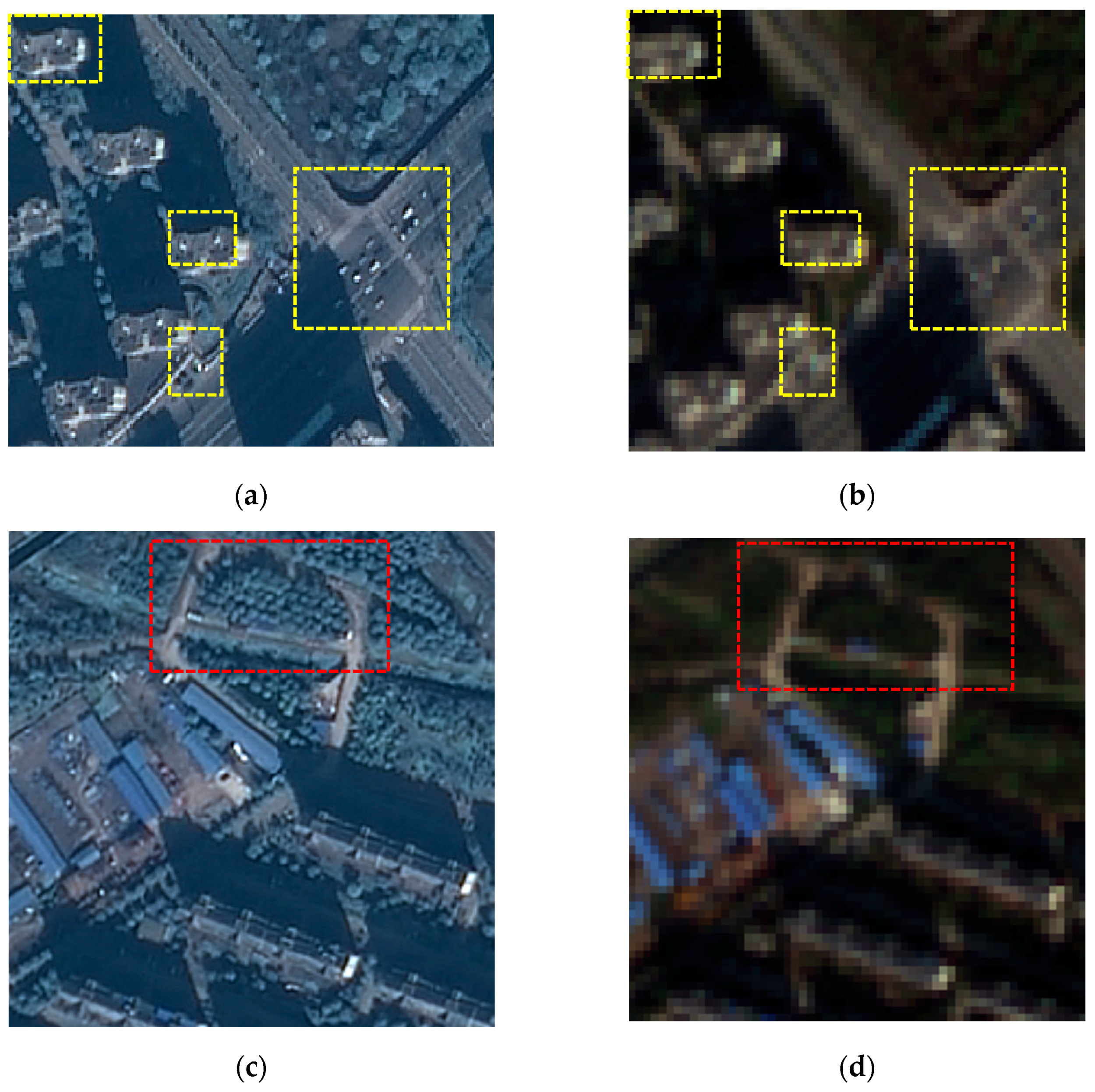
• Till now almost all datasets for VHRRSI are from aerial imagery which covers some regions in the US or Europe, with a good imaging condition. No VHRRSI dataset designed for Chinese region is available now, while urban and suburban landscapes in China and Western countries are quite different (examples are demonstrated in Figure 3). Note that it is acknowledged that different training samples usually lead to quite different performance for data-driven methods and that in many cases the imaging condition of satellite image is different from aerial images.
• No open VHRRSI building extraction dataset from satellite imagery is available now, let alone the requirement to fit into both model-driven and data-driven methods since for model-driven methods, the near infrared channel is quite important for their implementation and performance.

3. Methodology

3.1. Multi-Scale Building Index

Image filtering was first studied to remove noise and was then widely used to extract features in a series of visual tasks. Filtering can be divided into two categories, that is, linear filtering and nonlinear filtering. Average filtering is typical linear filtering while morphological operations belong to nonlinear filtering.

Inspired by the fact that average filtering is effective to remove noise and is of less computation cost, in this work, average filters are tested to generate Multi-scale building index (MFBI) for the extraction of building areas. Compared with MBI, multi-scale and multi-direction linear morphological filtering is replaced by multi-scale filtering, and the top-hat transformation in MBI is abandoned. In other words, with similar parameter settings of window size, all morphological operations are abandoned to alleviate computation cost. Instead, the average filter is implemented and it can overcome noise in VHRRSI.

As Figure 4 has demonstrated, the proposed MFBI has the following steps.

Step 1. The generation of brightness image $I\left(x\right)$. In MFBI, the brightness image is generated from each pixel’s maximal spectral value among three optical bands, as (1) expresses. Here, red, green and blue denote the red, green and blue band of an image respectively. The reason why we choose only optical bands is that recently it is reported that visual bands contribute significantly to the spectral property of building areas [55].

$$I\left(x\right)=\mathrm{Max}\left\{Red\left(x\right),Green\left(x\right),Blue\left(x\right)\right\}.$$

(1)

Step 2. The generation of filtering profiles. A series of filters with window sizes of an equal difference (parameters include initial window size $S_{\min }$, final window size $S_{\max }$ and step size $\Delta s$) on brightness image is applied. It should be noted that these parameter settings are similar to MBI in VHRRSI [50]. Here, FPavr and s denote filtering profiles of average filters and window size respectively. Let $\left(x,y\right)$ be a pixel of brightness image I, and i, j belong to an integer, we have:

$$F{P}_{avr}\left(s\right)=\frac{1}{s\times s}{\displaystyle \sum }_{\begin{array}{c}-\frac{s-1}{2}\le i\le \frac{s-1}{2}\\ -\frac{s-1}{2}\le j\le \frac{s-1}{2}\end{array}}I\left(x+i,y+j\right)$$

(2)

$$F{P}_{avr}=\left\{F{P}_{avr}\left(s\right),s\in \left\{S_{min},S_{min}+\Delta s,\cdots ,S_{max}-\Delta s,S_{max}\right\}\right\}.$$

(3)

Step 3. The generation of differential filtering profiles. After step 2, we can get k − 1 corresponding differential images. Here, k is calculated via $k=\left(S_{\max }-S_{\min }\right)/\Delta s+1$. Let DFPavr denote the differential filtering profile of average filters, and it can be expressed in Formula (4).

$$DF{P}_{avr}\left(s\right)=\left|F{P}_{avr}\left(s+\Delta s\right)-F{P}_{avr}\left(s\right)\right|$$

(4)

Step 4. The generation of MFBI. k − 1 corresponding differential images in step 3 are averaged and normalized into [0, 1] to generate MFBI.

$$\mathrm{MFBI}={\displaystyle \sum _{s=S_{\min }}^{S_{\max }}DFPavr\left(s\right)}/k$$

(5)

Step 5. Extraction of building areas. Similar to the extraction framework of MBI, after the generation of MFBI, the extraction of building areas are implemented according to a series of rule sets. Since the size of the original image and MFBI feature image is the same, let $\left(x,y\right)$ denote a pixel of the MFBI feature image. Then, it is segmented by the rule set defined in (6). Here, T denotes threshold value for MFBI.

$$\mathrm{MFBI}\left(x,y\right)>T$$

(6)

Step 6. Post processing framework. The image is composed of a series of segmented regions that could belong to building regions. Let NDVI, and T_NDVI denotes threshold value for NDVI of an image, and the NDVI segmentation value respectively. Meanwhile, Let l, Ratio, R₁, Area and A₁ denote such a region, the length-width ratio of such a region, the corresponding threshold of length-width ratio, the area and the corresponding threshold value of the area, the post-processing framework is composed of a series of operations denoted in the rule set (7). Note that the length-width ratio of each object is calculated via oriented bounding boxes so that objects at different orientations can be described more accurately.

$$\{\begin{array}{l}NDVI\left(x,y\right)<T_{NDVI}\\ Ratio\left(l\right)<R_1\\ Area\left(l\right)>A_1\end{array}.$$

(7)

A threshold value T is set to segment pixels that possibly belong to building areas. Due to the fact that the framework and operations of MFBI are similar to that of MBI, the threshold value of MFBI is similar to the threshold value of MBI, which has been carefully studied in References [34,51]. Pixels belonging to building areas usually have an MFBI between 0.4 and 0.6. The three operations in rule set (7) are strategies to remove the false alarms (e.g., removal of vegetation, elimination of elongated roads), similar to the implementation in References [34,51,58]. It should be noted that after the NDVI threshold, we first fill holes in the binary image and then we implement the second and the third operation in (7). Compared with the former works [34,50], filling holes before region selection can alleviate the problem that some parts of a building roof are excluded by calculating NDVI when these parts of a roof are covered by vegetation.

3.2. Joint Use of MFBI and Spectral Information

To fully and jointly utilize spectral and spatial information, two scenarios to extend MFBI to multiple channels (Multi-channel MFBI, MMFBI) are proposed in this paper, as is demonstrated in Figure 5. As is pointed in Section 3.1, related work has pointed out that visual bands contribute significantly to the spectral property of building areas [55].

To further discriminate the spectral information of building areas from others, principal component analysis (PCA) [59,60], one of the most commonly used methods to improve the feature separability, is implemented in these two scenarios.

Let z and x denote a lower dimension and higher dimension matrix respectively, PCA tends to find a mapping w which can present the relation between z and x.

$$z=w^{T}x.$$

(8)

The most paramount component $w_1$ satisfies the condition that after projected to $w_1$, samples become the most distinctive. Hence, we have:

$$Var\left(z_1\right)=E\left[{\left(w^{T}x-w^T\mu \right)}^2\right]=w_1{}^T{\displaystyle \sum w_1}.$$

(9)

The objective is to find and maximize $w_1$. It can be regarded as a Langulan problem, in the below form as the formula (9) is expressed:

$$\underset{w_1}{\max }{w}_1{}^T{\displaystyle \sum w_1-\alpha \left(w_1{}^T{w}_1-1\right)}.$$

(10)

With the utilization of PCA, two scenarios are described in detail as follows.

Scenario 1. Principal component analysis (PCA) is implemented on three visual bands (Red, Green and Blue) of VHRRSI. Then, information of the first component PC1(x) is regarded as the brightness image to generate MFBI feature image, since much information of the building areas has been transformed into PC1(x) after PCA.

Scenario 2. For each channel in the three channel RGB image, MFBI feature image is generated and a three channel MFBI image is obtained. Then, a principal component analysis is implemented on this three-channel MFBI feature image. We continue to step 3 and 4 on the first component PC1(x) of this feature image. Similarly, it is reported in Reference [48] that after texture-derived feature extraction, the first component is selected since it contains much signal of building regions. In our experiments, the first component also contains much signal from building areas.

4. Experiments and Analysis

4.1. Dataset

MBI was proposed to extract single building in imagery in HRRSI, especially effective in Chinese urban regions. As an improvement of MBI, MFBI is also capable of building extraction.

However, as is mentioned in Section 2.3, no open dataset for building extraction task in HRRSI is available now to compare these model-driven methods, while the aforementioned VHRRSI datasets sampled from Western countries are more appropriate for data-driven methods since they do not contain the near infrared channel which is of importance for many model-driven methods.

Hence, to fairly compare these model-driven methods like MBI and MFBI on VHRRSI, and to offer a benchmark for these algorithms’ performance on Chinese regions, an open dataset named Wuhan University Building Extraction Dataset (WHUDBE) is introduced in this paper (download link: https://drive.google.com/open?id=1TfyNPSRSs8jMtbeSiP90SbGLW7fhjj6z).

The consideration of selecting samples for the dataset mainly include the following aspects:

• The inter-class similarity and intra-class dissimilarity in VHRRSI. It is widely acknowledged that with the increase of spatial resolution, both the similarity between different types of land cover and the dissimilarity of the same type of land cover have largely increased, resulting in a series of problems for the automatic interpretation of VHRRSI. Hence, to test the performance of a specific algorithm, the variety of building shapes, building sizes and building roofs must be considered when selecting samples for our datasets.
• Land covers hard to be distinguished in the building extraction task. In Reference [61], Mohsen concludes that one of the major challenges in building extraction tasks in VHRRSI is the existence of shadow, vegetation, water regions, and man-made non-building features. These types of land cover should also appear in the samples of our datasets to test the performance of an algorithm.
• The covering of typical Chinese landscape in different regions as many as possible. It is known that different regions in China usually have different building structures due to a series of factors such as the influence of economy, climate, population and so on. Meanwhile, the urban, suburban and rural areas should also be covered.

31 pan-sharpened VHRRSI from 7 provinces in China are the data source of our dataset. These seven provinces come from the Eastern, North-western, Southern, and the middle Chinese regions respectively. Sensors include Quick Bird, Gaofen-2, WorldView2, with a spatial resolution of 0.6, 0.8 and 0.5 m respectively. Based on the principles mentioned above, we carefully choose 57 pieces of image patches with a row and column of 512 pixels and 512 pixels respectively to validate the performance of the proposed method. Figure 6 illustrates all the samples from our dataset. When choosing samples, effort has been made to present the complexity of building area landscape and to include those challenge elements mentioned in Reference [61] as much as possible. After that, ground truth is labeled by two experts who are not involved in our study.

When compared with the other two aforementioned VHRRSI building extraction datasets with our newly published dataset, several aspects are listed as follows. In terms of the data source, our dataset, all from VHRRS satellite imagery, serves as a good complementary of the other two aerial image datasets. In terms of the study region, our dataset can well represent the reality and complexity of the building areas among China, and can also be regarded as a good complementary for these two datasets covering America and Europe. More importantly, our dataset offers the near infrared band from the satellite sensors and thus can be utilized to validate both the model-driven and data-driven building extraction algorithms. Note that in Section 2.3, we have mentioned that the near infrared information is important for many model-driven building extraction methods.

4.2. Parameter Settings

In all experiments mentioned below, parameter settings for MBI and MFBI are listed in

Table 3. Parameter settings of MBI and MFBI.

	Smin	Step Size	Smax	Threshold
MBI	2	5	42	0.45
MFBI	3	6	33	0.45

. The most significant parameter for both MBI and MFBI is the segmentation threshold, which will be discussed later. The window size of profiles also has a strong influence on the effectiveness of extracted feature maps. For MBI, these window sizes are all set the same as Reference [50], while for MFBI a smaller maximum window size and a larger threshold value is needed. For the object-oriented-based method, we use eCognition to extract building regions. Allowing for the multiple scales of building areas, a 2-scale segmentation stratagem, with the scale parameters of 120 and 60 respectively, is implemented to segment image and the rule sets are the same as Huang did in Reference [34].

For the framework of post-processing, since this paper mainly pays attention to the development of MFBI and MMFBI, we do not fine-tune those parameters on our datasets. Instead, in all test images, NDVI to remove false alarms caused by vegetation, area threshold to remove small objects, and length-width ratio threshold to remove elongated roads, are set to be 0.1, 30, and 5.6, respectively, the same as Huang did in Reference [50]. It should be noted that since we do not fine-tune these parameters on our own dataset, there is much possibility that after the fine-tuning of parameters in the post-processing framework, MFBI could achieve a better accuracy on our dataset.

All of our experiments are implemented on a personal computer with CPU i5-7500 and RAM 8GB. All codes are programmed in Visual Studio 2015, with API from OpenCV3.0.

4.3. Experiments on Basic MFBIs

4.3.1. Experiment on Computation Time

Three large-scale VHRRSIs are chosen to test the computation time of MBI and MFBI. The basic information of these images (i.e., image size, sensor type, spatial resolution) and computation time are listed in

Table 4. Computation time of MBI and MFBI on three large-scale images.

	Image Size (in Pixel)	Spatial Resolution (in Meters)	Sensors	Computation Time of MBI (in Seconds)	Computation Time of MFBI (in Seconds)
Image1	15392 × 16384	0.6	Quick Bird	2177.76	26.91
Image2	16384 × 16384	0.5	World View 2	1565.07	29.03
Image3	19464 × 18573	0.8	Gaofen 2	2191.13	38.49

. In Figure 7, these three images, the corresponding MBI and MFBI feature map are demonstrated. Note that some false alarms caused by vegetation have been removed via calculating NDVI in these feature maps.

From Table 4, we can observe that the proposed MFBI outperforms MBI with much less computation time on large scale satellite images. From Figure 7, in terms of visual effect, in many regions of these feature maps, MFBI are more capable of preserving features of building areas than MBI with less noise, while MBI could cause cracks on building roofs. It can be explained by the fact that average filtering is more capable of generating homogeneous regions with similar gray values while multi-scale and multi-direction morphological operations could lead to the exclusion of a few pixels in the building roof due to their different gray value.

4.3.2. Experiments on WHUBED

The developed MFBI are compared with MBI and the widely used object-oriented segmentation method on our newly published WHUBED. In this section, we will compare them from both the visual effect and quantitative analysis.

In Figure 8, the extraction results and the corresponding ground truth maps of four samples from different landscapes are demonstrated for the comparison of visual effect. The first row is the original images, the second row is the corresponding ground truth maps, and from the third to the seventh row, the extraction results of the object based segmentation method, MBI, MFBI, the first scenario of MMFBI and the second scenario of MMFBI are listed respectively. Although these four samples look simple at a first glance, they are challenging if a relatively high accuracy can be obtained mainly because of the following characteristics.

Sample 1: On the upper area, several informal settlements are located and on the right of the lower area, several buildings with a dark roof are located. Note that for MBI, two weaknesses lie in the incapable of extracting informal settlements and the dark built-up regions [34]. Meanwhile, on the left of the lower region, the wide road and the boat on the river is also easy to introduce false alarms.

Sample 2: The difficulty lies in the imaging condition and the land covers on the river bank. Under this unsatisfactory imaging condition, ground objects on the image are a little bit obscure. The bright and wide roads and other man-made objects are easy to cause false alarms.

Sample 3: The difficulty lies in the low intensity of the image and the dark building roofs of the informal settlements. As is mentioned in Sample 1, these two problems are challenging for MBI. Since the elongated road can be easily eliminated by the morphological operations, it should not be considered as difficult as some former researchers do.

Sample 4: Building areas are relatively small in size and are irregular in geometry, tending to cause omission errors. Meanwhile, the texture from the farmland and the road makes it easier to introduce false alarms.

In terms of the visual effect, those informal settlements and building in small sizes are more effectively extracted in these samples with our proposed MFBI and the false alarms introduced by road or other small man-made objects are relatively less, when compared to other methods. These better-performed regions are marked by red bounding boxes in Figure 8.

For accuracy assessment, we choose the commonly used recall, precision and F1-score for the assessment of building extraction tasks as our measurement to evaluate the performance of building extraction results [45,62]. Usually, recall reflects an algorithm’s ability to find true positives, while precision reflects an algorithm’s cost to find true positives. In addition, F1-score measures the ability of both precision and recall.

$$precision=\frac{tp}{tp+fp}$$

(11)

$$recall=\frac{tp}{tp+fn}$$

(12)

$$F1=2\times \frac{precision\times recall}{precision+recall}$$

(13)

where tp, fp, tn, and fn denote true positive, false positive, true negative and false negative, respectively.

The accuracy of three building extraction methods on every sample in our dataset is listed in

Table 5. Accuracy of the proposed MFBI and two scenarios of Multi-channel MFBI (MMFBI) compared with MBI and eCognition on WHUBED (in percentage). Note that: R, P and F denote recall, precision and F1-score respectively. eC, S1 and S2 denote the multi-scale segmentation based method operated on eCognition, Scenario 1 and Scenario 2 of MMFBI respectively. The best performance of the recall, precision and F1-score on each sample is marked bold.

		R	P	F			R	P	F			R	P	F
Sample1	eC	58.04	61.53	61.53	Sample2	eC	60.74	66.74	63.60	Sample3	eC	50.25	80.72	61.94
	MBI	65.79	73.81	69.57		MBI	80.41	63.60	71.02		MBI	61.03	76.55	67.92
	MFBI	94.87	68.58	79.61		MFBI	96.99	60.56	74.56		MFBI	90.93	68.17	77.92
	S1	92.82	70.57	80.18		S1	92.92	67.02	77.87		S1	84.24	75.61	79.69
	S2	93.56	70.91	80.68		S2	91.29	64.26	75.42		S2	88.06	72.02	79.23
Sample4	eC	58.08	79.08	66.97	Sample5	eC	57.23	62.27	59.64	Sample6	eC	67.95	38.70	49.32
	MBI	83.22	74.21	78.46		MBI	69.13	78.72	73.61		MBI	88.85	70.85	78.84
	MFBI	95.86	71.99	82.23		MFBI	82.49	72.10	76.95		MFBI	98.57	67.62	80.21
	S1	95.69	73.91	83.40		S1	95.52	74.82	83.91		S1	95.29	71.51	81.70
	S2	94.28	68.29	79.21		S2	96.21	73.66	83.41		S2	96.17	69.58	80.74
Sample7	eC	62.29	74.12	67.69	Sample8	eC	64.04	38.74	48.27	Sample9	eC	48.00	30.61	37.38
	MBI	83.87	73.09	78.11		MBI	81.92	69.08	74.95		MBI	65.72	74.95	70.03
	MFBI	97.65	68.10	80.24		MFBI	91.10	67.45	77.51		MFBI	89.68	66.98	76.69
	S1	94.63	71.56	81.49		S1	91.45	68.28	78.19		S1	85.18	71.43	77.70
	S2	92.67	73.04	81.69		S2	91.87	67.25	77.65		S2	85.27	70.49	77.18
Sample10	eC	54.75	45.91	49.94	Sample11	eC	47.61	36.29	41.19	Sample12	eC	29.97	39.38	34.04
	MBI	67.23	74.18	70.53		MBI	67.59	74.18	70.73		MBI	67.01	71.98	69.40
	MFBI	88.37	69.77	77.97		MFBI	81.25	63.93	71.56		MFBI	87.57	66.64	75.69
	S1	85.11	72.02	78.02		S1	79.61	71.77	75.48		S1	83.39	68.58	75.26
	S2	85.97	74.45	79.80		S2	79.73	70.97	75.09		S2	82.04	69.15	75.05
Sample13	eC	22.10	28.71	24.98	Sample14	eC	54.33	45.71	49.65	Sample15	eC	53.46	61.00	56.98
	MBI	51.03	65.94	57.53		MBI	74.65	82.15	78.22		MBI	78.44	72.54	75.37
	MFBI	62.21	59.94	61.05		MFBI	84.25	76.98	80.45		MFBI	89.15	68.90	77.73
	S1	67.82	59.87	63.59		S1	86.74	78.04	82.16		S1	90.20	70.49	79.14
	S2	68.75	57.91	62.86		S2	86.48	78.67	82.39		S2	89.78	70.39	78.91
Sample16	eC	51.41	37.26	43.21	Sample17	eC	56.72	48.63	52.36	Sample18	eC	78.38	59.81	67.85
	MBI	71.42	77.76	74.45		MBI	79.48	73.98	76.63		MBI	67.88	78.00	72.59
	MFBI	89.30	70.40	78.73		MFBI	88.00	68.60	77.10		MFBI	87.65	71.19	78.56
	S1	88.64	76.51	82.13		S1	89.07	67.22	76.62		S1	86.62	77.20	81.64
	S2	89.85	79.51	84.36		S2	87.19	74.16	80.15		S2	86.65	76.47	81.24
Sample19	eC	69.99	28.71	40.72	Sample20	eC	56.30	47.88	51.75	Sample21	eC	58.89	47.81	52.77
	MBI	68.50	71.00	69.73		MBI	71.86	70.56	71.20		MBI	73.49	74.35	73.91
	MFBI	91.21	65.84	76.48		MFBI	87.78	67.15	76.09		MFBI	89.57	67.09	76.72
	S1	90.56	68.06	77.71		S1	87.66	69.93	77.79		S1	90.07	66.96	76.81
	S2	90.15	69.40	78.43		S2	87.08	68.36	76.59		S2	87.05	72.14	78.90
Sample22	eC	72.56	46.72	56.84	Sample23	eC	76.57	63.26	69.28	Sample24	eC	79.11	38.45	51.74
	MBI	82.17	66.67	73.61		MBI	59.98	74.24	72.04		MBI	73.56	75.01	74.28
	MFBI	91.58	66.97	77.37		MFBI	89.80	71.21	79.43		MFBI	99.38	65.64	79.06
	S1	91.31	76.38	83.18		S1	89.36	74.57	81.30		S1	97.97	69.57	81.36
	S2	91.75	75.46	82.82		S2	89.12	78.10	83.24		S2	98.10	70.72	82.19
Sample25	eC	48.90	50.61	49.74	Sample26	eC	57.06	48.44	52.39	Sample27	eC	57.32	50.83	53.88
	MBI	69.50	78.89	73.90		MBI	70.58	69.24	69.91		MBI	83.81	78.33	80.98
	MFBI	80.40	74.52	77.35		MFBI	82.51	65.83	73.23		MFBI	89.04	73.21	80.35
	S1	84.03	73.01	78.14		S1	82.02	72.20	76.80		S1	88.27	77.44	82.50
	S2	83.99	73.33	78.30		S2	81.60	68.28	74.35		S2	89.72	76.40	82.53
Sample28	eC	48.22	60.16	53.53	Sample29	eC	58.40	53.60	55.90	Sample30	eC	49.12	73.77	58.98
	MBI	67.27	75.79	71.28		MBI	63.53	79.05	70.44		MBI	72.88	78.89	75.77
	MFBI	80.37	71.41	75.63		MFBI	89.66	69.53	78.32		MFBI	88.14	75.59	81.38
	S1	76.44	75.90	76.17		S1	84.32	79.76	81.98		S1	88.34	78.55	83.16
	S2	75.96	75.85	75.91		S2	88.27	74.63	80.88		S2	89.06	76.86	82.51
Sample31	eC	56.11	59.01	57.52	Sample32	eC	61.19	65.94	63.48	Sample33	eC	72.82	52.61	61.09
	MBI	76.51	73.36	74.90		MBI	71.91	79.62	75.57		MBI	70.44	83.30	76.33
	MFBI	88.16	66.14	75.58		MFBI	86.84	71.49	78.42		MFBI	89.44	76.37	82.39
	S1	88.85	75.78	81.80		S1	87.06	83.72	85.35		S1	88.73	79.30	83.75
	S2	87.55	68.25	76.70		S2	89.62	77.81	83.30		S2	88.07	78.53	83.02
Sample34	eC	74.07	52.79	61.64	Sample35	eC	80.10	43.14	56.08	Sample36	eC	80.59	37.43	51.12
	MBI	76.83	73.54	75.15		MBI	67.27	72.60	69.83		MBI	72.95	76.43	74.65
	MFBI	86.08	68.21	76.11		MFBI	99.51	66.15	79.47		MFBI	86.77	70.91	78.05
	S1	88.60	74.13	80.72		S1	95.27	69.37	80.28		S1	90.63	74.12	81.55
	S2	87.67	72.51	79.37		S2	96.79	68.11	79.95		S2	91.48	75.73	82.86
Sample37	eC	57.76	32.30	41.43	Sample38	eC	55.72	14.68	23.24	Sample39	eC	69.03	42.90	52.91
	MBI	67.96	61.47	64.55		MBI	62.78	78.75	69.86		MBI	73.81	75.64	74.71
	MFBI	84.26	59.77	69.93		MFBI	91.79	72.90	81.27		MFBI	89.36	67.93	77.17
	S1	96.08	61.34	71.63		S1	90.79	75.81	82.63		S1	87.07	72.89	79.35
	S2	93.71	65.27	73.35		S2	89.65	76.20	82.38		S2	89.58	71.54	79.55
Sample40	eC	74.53	70.15	72.27	Sample41	eC	30.80	50.63	38.30	Sample42	eC	63.55	57.60	60.43
	MBI	70.27	75.49	72.79		MBI	70.12	80.87	75.11		MBI	72.90	78.38	75.54
	MFBI	87.93	76.63	81.89		MFBI	83.54	75.48	79.31		MFBI	87.49	74.73	80.61
	S1	85.21	79.09	82.04		S1	89.09	79.42	84.43		S1	85.94	78.09	81.83
	S2	86.25	78.28	82.07		S2	89.41	77.84	83.22		S2	84.74	78.67	81.59
Sample43	eC	17.31	71.80	27.89	Sample44	eC	16.82	29.49	21.42	Sample45	eC	25.13	80.99	38.36
	MBI	53.10	84.99	65.36		MBI	64.57	73.27	68.65		MBI	51.31	76.92	61.56
	MFBI	83.84	63.69	72.39		MFBI	86.20	62.23	72.28		MFBI	84.64	57.90	68.76
	S1	81.14	67.22	73.53		S1	84.92	67.14	74.99		S1	83.07	62.96	71.63
	S2	83.87	66.04	73.90		S2	84.30	64.62	73.16		S2	81.59	62.77	70.95
Sample46	eC	18.32	32.48	23.43	Sample47	eC	25.65	82.17	39.10	Sample48	eC	18.18	73.89	29.18
	MBI	57.13	75.22	64.94		MBI	64.47	75.01	69.34		MBI	54.29	89.63	67.63
	MFBI	76.81	60.92	67.95		MFBI	84.66	65.31	73.73		MFBI	82.67	74.86	78.57
	S1	75.50	69.17	72.20		S1	86.06	72.31	78.59		S1	82.08	80.50	81.28
	S2	73.27	91.74	72.50		S2	84.51	73.38	76.80		S2	83.24	81.95	82.59
Sample49	eC	10.52	53.07	17.56	Sample50	eC	12.53	31.65	17.95	Sample51	eC	72.11	59.17	65.00
	MBI	57.77	78.54	66.57		MBI	61.63	67.97	64.64		MBI	57.31	67.44	61.96
	MFBI	83.77	73.91	78.53		MFBI	86.69	61.76	72.13		MFBI	91.41	60.81	73.04
	S1	84.79	75.24	79.73		S1	85.98	63.98	73.37		S1	88.27	65.04	74.90
	S2	84.53	76.68	80.41		S2	86.87	65.68	74.81		S2	86.56	87.04	95.56
Sample52	eC	57.25	12.38	20.36	Sample53	eC	48.18	31.88	38.37	Sample54	eC	32.27	42.69	36.76
	MBI	59.12	70.96	64.50		MBI	55.59	68.97	61.56		MBI	63.10	70.80	66.73
	MFBI	86.45	69.12	76.82		MFBI	86.12	61.35	71.66		MFBI	68.92	73.02	70.91
	S1	88.68	73.98	80.67		S1	85.11	64.12	73.13		S1	68.72	75.86	72.12
	S2	85.55	75.55	80.24		S2	85.31	64.67	73.57		S2	67.04	78.99	72.53
Sample55	eC	47.30	38.74	42.59	Sample56	eC	68.94	57.28	62.57	Sample57	eC	42.83	46.80	38.05
	MBI	62.09	72.35	66,83		MBI	64.33	75.65	69.54		MBI	53.71	65.98	59.22
	MFBI	83.47	65.33	73.29		MFBI	75.12	64.81	69.58		MFBI	78.26	60.83	68.46
	S1	82.80	68.48	74.96		S1	81.99	66.55	73.47		S1	83.71	67.99	75.04
	S2	82.25	68.10	74.51		S2	82.31	67.02	73.88		S2	85.17	66.04	74.40

. In addition, the mean and standard deviation of these three indices of all 57 samples in WHUBED is listed in

Table 6. Mean and standard deviation of several methods compared on WHUBED (in percentage).

	Recall	Precision	F1-Score
eCognition	53.40 ± 19.37	50.21 ± 16.43	48.40 ± 14.47
MBI	68.51 ± 8.84	74.40 ± 5.17	70.93 ± 5.15
MFBI	86.94 ± 6.67	68.15 ± 4.87	76.22 ± 4.22
MMFBI Scenario1	86.71 ± 5.80	72.15 ± 5.21	78.60 ± 4.19
MMFBI Scenario2	86.64 ± 5.93	71.87 ± 5.10	78.40 ± 4.16

. From these results, some important observation can be found:

• For most of the samples in our dataset, the proposed MFBI achieves the highest F1-score and recall, while MBI tends to have higher precision (see Table 5). From Table 6, both MBI and the proposed MFBI can outperform the widely used object-oriented method.
• From the perspective of performance on different types of samples, all of the three methods, namely, objected based segmentation, MBI and MFBI, tend to perform better on urban or suburban areas. It can be explained that in these regions, many buildings are in regular shape while roads, one of the main false alarms, can be easily removed by post-processing when calculating shape index and length-width ratio. However, although MFBI performs better than the other two methods on rural areas, neither of these three methods are robust enough on rural areas, where the farmland with a regular geometric shape and too much bright bare soil can cause severe false alarms.
• The proposed MFBI tends to have relatively high recall and the precision value is lower than the recall value. The high recall and relatively high false alarm of MFBI might be explained by the utilization of rectangular filtering windows. Rectangular filters tend to stress the influence of bright pixels belonging to building areas but pixels around the building areas could also have a high gray value after calculating MFBI. In other words, the rectangular filtering window might not fully utilize the abundant spatial information of building areas in VHRRSI.

4.3.3. Sensitivity Analysis

As is mentioned in Section 3.1, sharing a similar framework and operation, the threshold value of MFBI and MBI tends to be similar. While the influence of MBI’s segmentation threshold value T has been carefully studied in References [34,50], in this section, we illustrate the influence of MFBI’s segmentation threshold value T on the results of building extraction.

Different light conditions and landscapes are taken into account for the illustration. Four samples, from different lighting conditions (i.e., bright, moderate and dark) while including different landscapes (i.e., urban regions, suburban regions and rural regions) are demonstrated in Figure 9. In the first and the second column of Figure 9, we demonstrate the samples and the corresponding MFBI feature map. In the third column of Figure 9, we offer the relation between different MFBI threshold and the corresponding recall, precision and F-score. From these figures, the observation is in accordance with the conclusion in References [34,50].

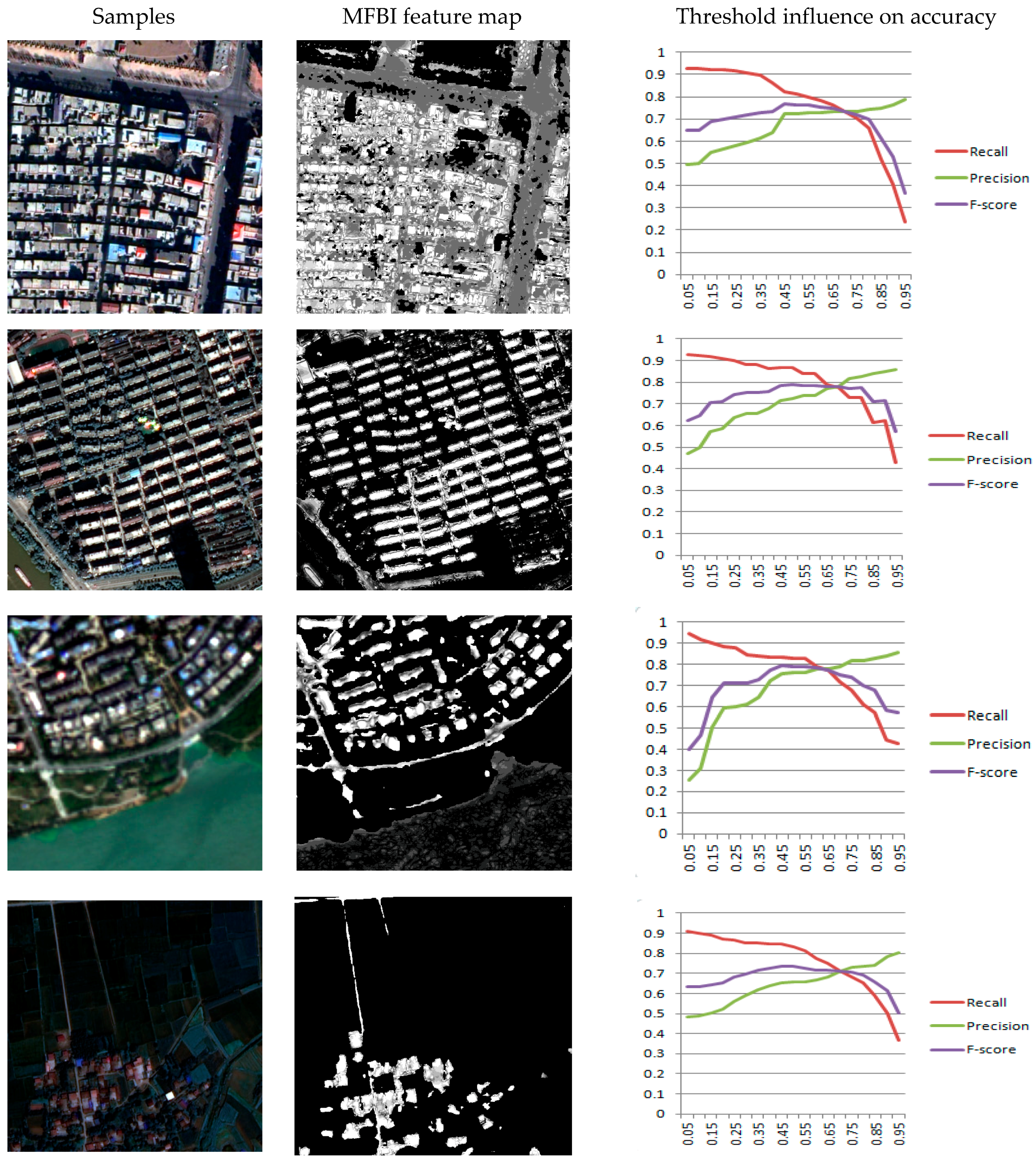
• With the increase of MFBI, the F-score tends to increase first and then decrease. While the recall tends to decrease, the precision tends to increase. This trend fits the general regulation of the recall and precision curves offered in References [34,50]. A small threshold usually leads to the selection of a relatively large amount of samples. Although we will get a high recall from these samples, a large number of false positives are among these samples, leading to the relatively low precision. On the contrary, when the threshold is set high, the algorithm will select a relatively small number of samples with relatively high precision, while some true positives are missed.
• When the threshold is set from 0.4 to 0.6, the proposed method can usually achieve the best performance with a high recall value and a modest precision value, no matter in urban, suburban or rural regions. It can be explained that after the feature extraction of MFBI, pixels belonging to building areas often have an MFBI value at about 0.4 to 0.6. Such regulation has also been reported in Reference [34].

4.4. Experiments on Two Proposed Scenarios

Before discussing the extraction results of MMFBI, we first demonstrate and discuss the feature map of these two scenarios to generate MMFBI. In Figure 10, the results after PCA in the first and the second scenario to generate MMFBI are demonstrated. As is mentioned in Section 3.2, we choose the first component of these results (these results are shown in the second and third component of Figure 10) to get the MMFBI feature maps for building extraction. From these results we can observe that:

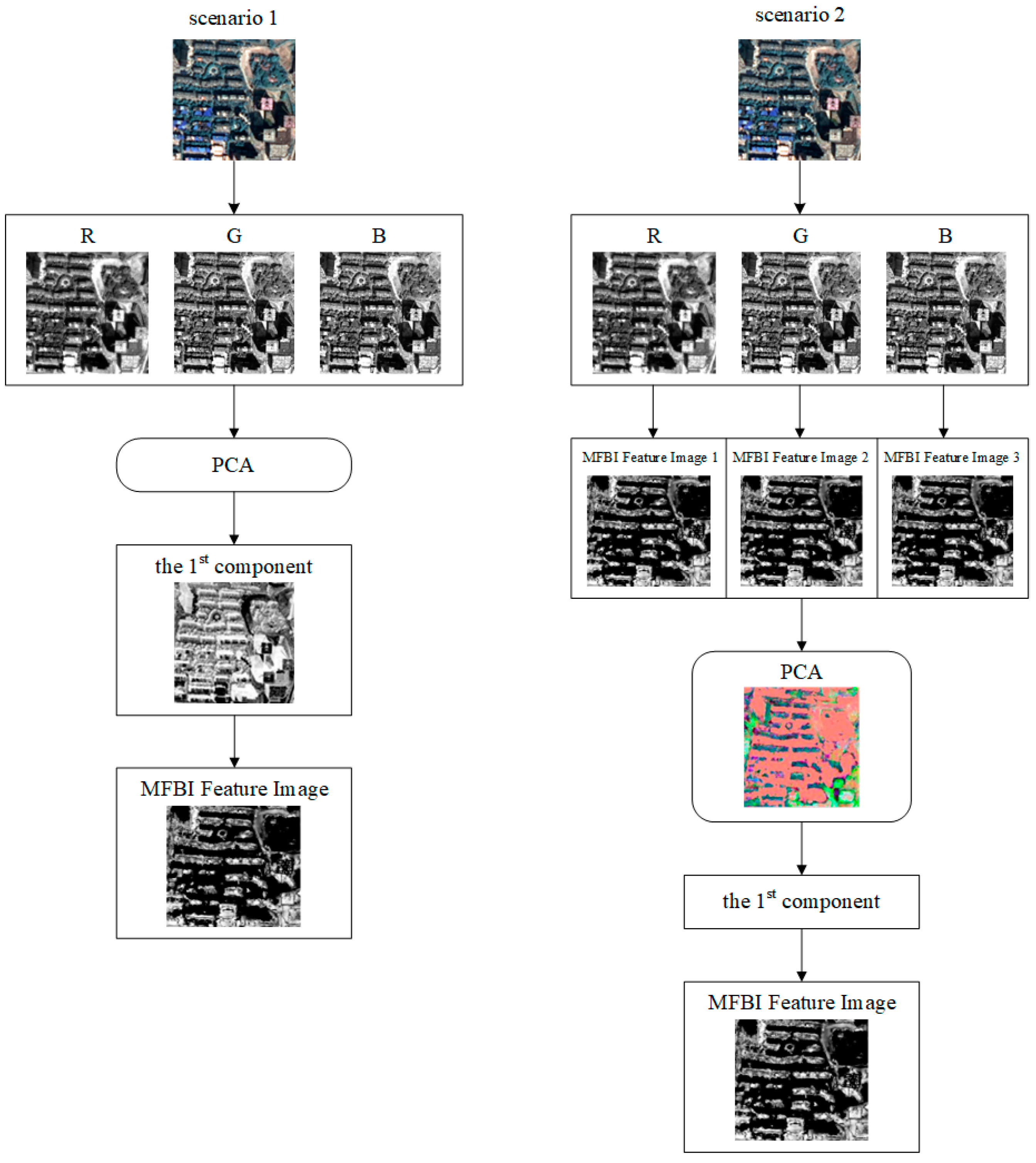
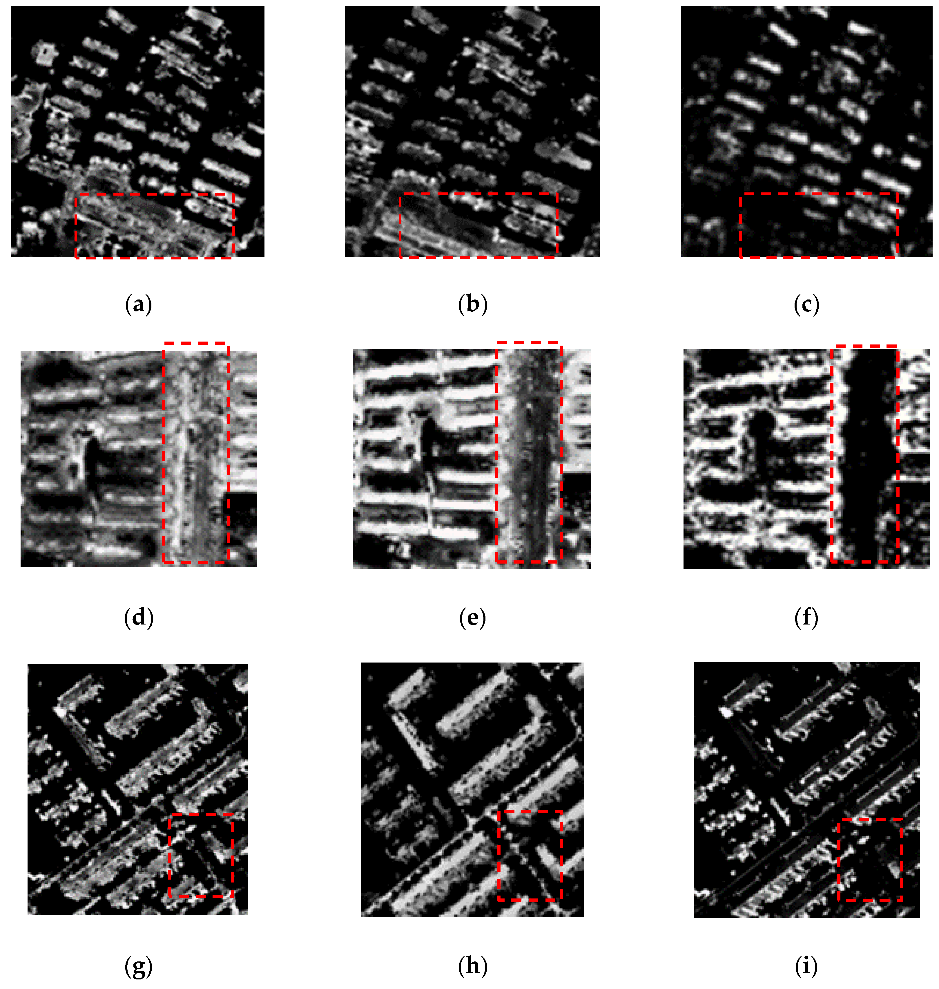
• The implementation of PCA can help extract building features. In the first scenario, the PCA is implemented on the original image from our datasets. Much of the information from building pixels can be enhanced (see from the second column of Figure 10) and these homogenous regions are salient in the first component.
• For the second scenario to generate MMFBI, after the calculation of MFBI in each channel and the PCA transformation, the MMFBI feature map is more capable to enhance building areas than the MMFBI feature map in our first scenario, which simply implements PCA on optical images. It can be explained that the calculation of MFBI on each channel selects pixels that could belong to building areas and later PCA refines these selected pixels. For example, some pixels belonging to vegetation are selected in the red channel but are not selected in the green and blue channel, and the PCA implementation can exclude these pixels from the feature map.

The proposed two scenarios in Section 3.2 are tested on our dataset and their performance on each sample is listed in Table 5. And the mean and standard deviation of these three indices of all 57 samples in WHUBED is listed in Table 6. From these results, we can observe that:

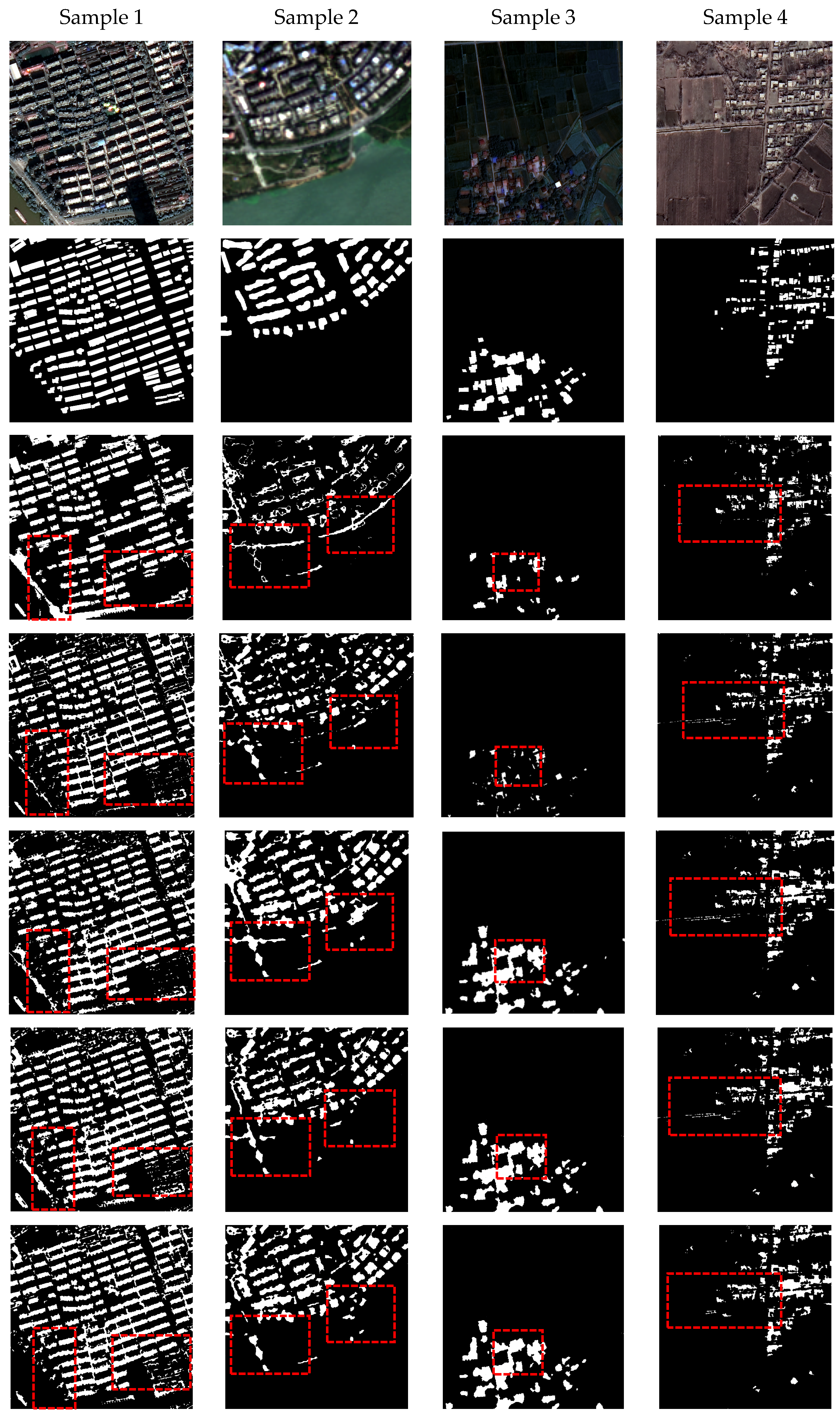
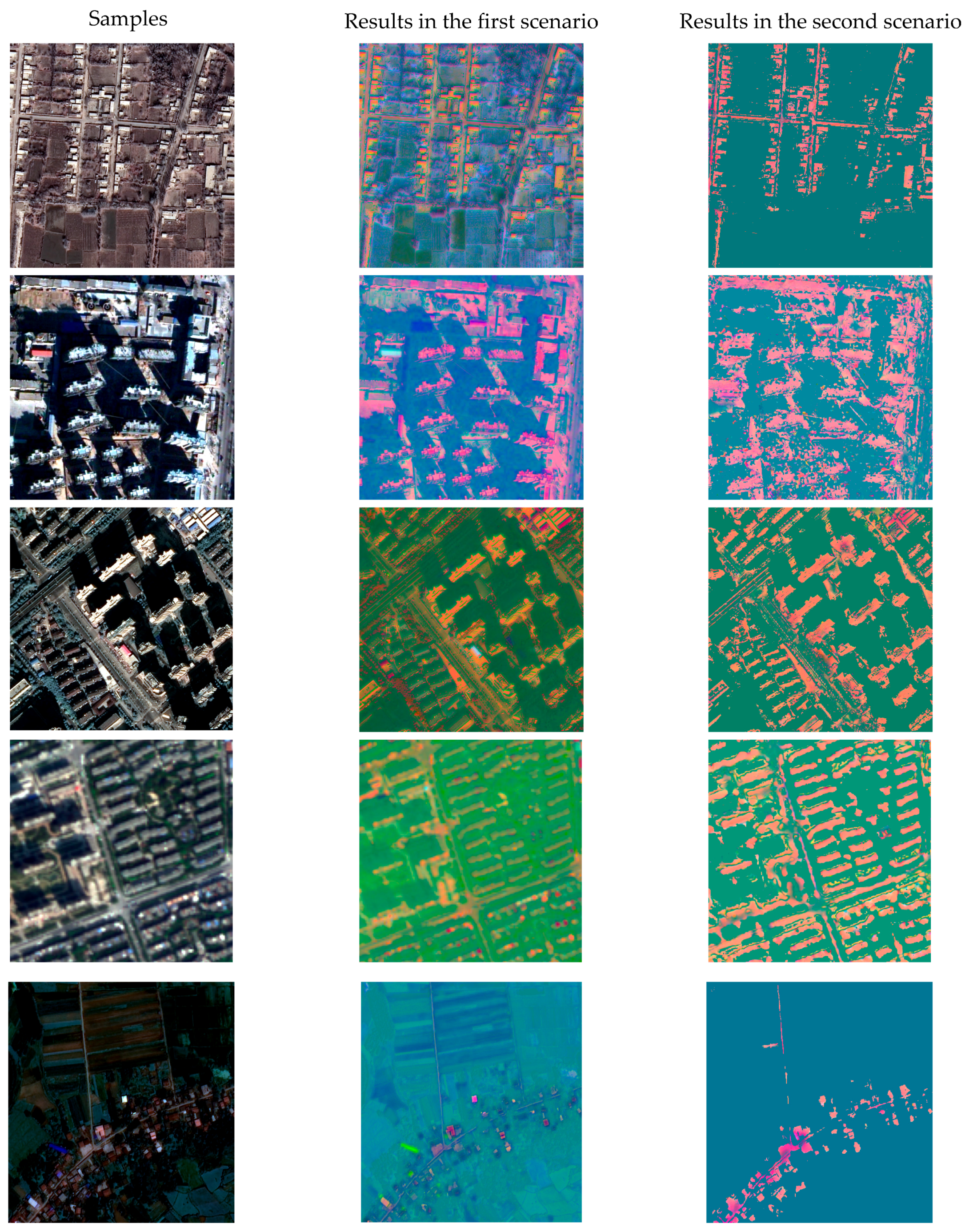
• The feature extraction ability of the two proposed scenarios is better than the basic MFBI, especially when we take account of the precision and the F-score. This result is reasonable since information that contributes greatly to building areas and other man-made objects in the red, green and blue channel are all taken into account and the signal of some false alarms from one single channel can be suppressed. This phenomenon is clearly demonstrated in Figure 8 and Figure 11. From the sixth and seventh row of Figure 8 and the first column of Figure 11, much noise mainly from wide roads can be observed in the MFBI feature map, while in the second and the third column of Figure 11, noise is much less in the MMFBI feature maps.
• The first scenario can make the feature map more compactness since the first component of the three channel optical image contains more information on the building structures while suppresses much information from other types of land cover. This phenomenon is clearly demonstrated in the second row of Figure 11.
• The second scenario can improve the accuracy mainly because of the calculation of MFBI on three channels separately and PCA transformation after that. Calculating MFBI on each channel makes full use of information that can present the signal of building areas and the PCA transformation on this image can refine the result by eliminating some pixels belonging to other land ground types such as road or bare soil. The situation that some roads mixed with building areas in the feature map of MFBI and the first scenario of MMFBI can be removed in the feature map of the second scenario MMFBI is obvious in the image of Figure 11c,f,i. Meanwhile, as is mentioned in Section 3.2, after PCA, while the first component contains much signal from building areas, the second component contains much information from other land covers such as roads and bare soil. However, simply using the second component also takes the risk of excluding some building areas whose material is similar to roads. It should be emphasized that in pixel-level building detection, one of the major differences between HRRSI and VHRRSI is that roads are much wider in VHRRSI and are more difficult to be eliminated.

5. Conclusions

In this paper, a multi-scale filtering building index (MFBI) is proposed with the objective to avoid complex morphological operations and use basic average filters instead. After a detailed study of current datasets for building extraction, in the hope of offering a VHRRSI dataset for model-driven based methods, we introduce our newly published dataset WHUBED and use it as a benchmark to compare our proposed method with the widely used object-oriented method and MBI. Experiments demonstrate that the proposed MFBI can generate building feature maps much faster than MBI, and can outperform the other two methods in terms of accuracy. To fully utilize spectral information that contributes to urban regions in VHRRSI, two scenarios to extend MFBI into multiple channels (MMFBI) are studied. Related experiments demonstrate that these two scenarios can reduce false alarms in MFBI and therefore can achieve higher accuracy.

However, some weaknesses for the proposed MFBI include: (1) It does not fully utilize spatial information especially multi-direction structural information, and can introduce artefacts. (2) The brightness image might not truly present building features when a sensor is too sensitive at many pixels in a particular channel.

Feature work includes the implementation of MFBI’s post-processing framework systematically and the utilization of more directional and structural information in MFBI.

References

1. Huang, X.; Wen, D.W.; Li, J.Y.; Qin, R.J. Multi-level monitoring of subtle urban changes for the megacities of China using high-resolution multi-view satellite imagery. Remote Sens. Environ. 2017, 56, 56–75. [Google Scholar] [CrossRef]
2. Joshi, N.; Baumann, M.; Ehammer, A.; Fensholt, R.; Grogan, K.; Hostert, P.; Jepsen, M.R.; Kuemmerle, T.; Meyfroidt, P.; Mitchard, E.T.A.; et al. A Review of the Application of Optical and Radar Remote Sensing Data Fusion to Land Use Mapping and Monitoring. Remote Sens. 2016, 8, 70. [Google Scholar] [CrossRef]
3. Zhang, T.; Huang, X. Monitoring of Urban Impervious Surfaces Using Time Series of High-Resolution Remote Sensing Images in Rapidly Urbanized Areas: A Case Study of Shenzhen. IEEE J. Sel. Top. Appl. Earth Observ. Remote Sens. 2018, 11, 2692–2708. [Google Scholar] [CrossRef]
4. Herold, M.; Goldstein, N.C.; Clarke, K.C. The spatiotemporal form of urban growth: Measurement, analysis and modeling. Remote Sens. Environ. 2003, 86, 286–302. [Google Scholar] [CrossRef]
5. Shen, J. Estimating Urbanization Levels in Chinese Provinces in 1982—2000. Int. Stat. Rev. 2006, 74, 89–107. [Google Scholar] [CrossRef]
6. Yew, C.P. Pseudo–Urbanization? Competitive government behavior and urban sprawl in China. J. Contemp. China 2012, 21, 281–298. [Google Scholar] [CrossRef]
7. Zhu, Y.G.; Ioannidis, J.P.; Li, H.; Jones, K.C.; Martin, F.L. Understanding and harnessing the health effects of rapid urbanization in China. Environ. Sci. Technol. 2011, 45, 5099–5104. [Google Scholar] [CrossRef] [PubMed]
8. Ji, C.Y.; Liu, Q.H.; Sun, D.F.; Wang, S.; Lin, P.; Li, X.W. Monitoring urban expansion with remote sensing in China. Int. J. Remote Sens. 2001, 22, 1441–1455. [Google Scholar] [CrossRef]
9. Zhang, Y. Optimisation of building detection in satellite images by combining multispectral classification and texture filtering. ISPRS J. Photogramm. Remote Sens. 1999, 54, 50–60. [Google Scholar] [CrossRef]
10. Mayer, H. Automatic Object Extraction from Aerial Imagery—A Survey Focusing on Buildings. Comput. Vis. Image Underst. 1999, 74, 138–149. [Google Scholar] [CrossRef]
11. Harris, R. Satellite remote sensing: Low spatial resolution. Prog. Phys. Geogr. 1995, 9, 600–606. [Google Scholar] [CrossRef]
12. Haala, N.; Kada, M. An update on automatic 3D building reconstruction. ISPRS J. Photogramm. Remote Sens. 2010, 65, 570–580. [Google Scholar] [CrossRef]
13. Thomas, M. Remote Sensing and Image Interpretation; John Wiley & Sons: Hoboken, NJ, USA, 1979. [Google Scholar]
14. Cheng, G.; Han, J.W. A Survey on Object Detection in Optical Remote Sensing Images. ISPRS J. Photogramm. Remote Sens. 2016, 117, 11–28. [Google Scholar] [CrossRef]
15. Han, X.; Zhong, Y.; Zhang, L. An Efficient and Robust Integrated Geospatial Object Detection Framework for High Spatial Resolution Remote Sensing Imagery. Remote Sens. 2017, 9, 666. [Google Scholar] [CrossRef]
16. Qiu, S.H.; Wen, G.J.; Liu, J.; Deng, Z.P.; Fan, Y.X. Unified Partial Configuration Model Framework for Fast Partially Occluded Object Detection in High–Resolution Remote Sensing Images. Remote Sens. 2018, 10, 464. [Google Scholar] [CrossRef]
17. Xu, Z.Z.; Xu, X.; Wang, L.; Yang, R.; Pu, F.L. Deformable ConvNet with Aspect Ratio Constrained NMS for Object Detection in Remote Sensing Imagery. Remote Sens. 2017, 9, 1312. [Google Scholar] [CrossRef]
18. Awrangjeb, M. Effective Generation and Update of a Building Map Database through Automatic Building Change Detection from LiDAR Point Cloud Data. Remote Sens. 2015, 7, 14119–14150. [Google Scholar] [CrossRef]
19. Barragán, W.; Campos, A.; Sanchez, G. Automatic Generation of Building Mapping Using Digital, Vertical and Aerial High Resolution Photographs and LIDAR Point Clouds. ISPRS Int. Arch. Photogramm. Remote Sens. Spat. Inf. Sci. 2016, XLI-B7, 171–176. [Google Scholar]
20. Tu, J.H.; Li, D.R.; Feng, W.Q.; Han, Q.H.; Sui, H.G. Detecting Damaged Building Regions Based on Semantic Scene Change from Multi–Temporal High–Resolution Remote Sensing Images. ISPRS Int. J. Geo-Inf. 2017, 6, 131. [Google Scholar] [CrossRef]
21. Dong, L.G.; Shan, J. A comprehensive review of earthquake-induced building damage detection with remote sensing techniques. ISPRS J. Photogramm. Remote Sens. 2013, 84, 85–99. [Google Scholar] [CrossRef]
22. Zhao, B.; Zhong, Y.F.; Zhang, L.P. A spectral-structural bag-of-features scene classifier for very high spatial resolution remote sensing imagery. ISPRS J. Photogramm. Remote Sens. 2016, 116, 73–85. [Google Scholar] [CrossRef]
23. Zhong, Y.F.; Zhu, Q.Q.; Zhang, L.P. Scene Classification Based on the MultiFeature Fusion Probabilistic Topic Model for High Spatial Resolution Remote Sensing Imagery. IEEE Trans. Geosci. Remote Sens. 2015, 53, 6207–6222. [Google Scholar] [CrossRef]
24. Csillik, O. Fast Segmentation and Classification of Very High Resolution Remote Sensing Data Using SLIC Superpixels. Remote Sens. 2017, 9, 243. [Google Scholar] [CrossRef]
25. Demir, B.; Bruzzone, L. Histogram–Based Attribute Profiles for Classification of Very High Resolution Remote Sensing Images. IEEE Trans. Geosci. Remote Sens. 2016, 54, 2096–2107. [Google Scholar] [CrossRef]
26. Pesaresi, M.; Benediktsson, J.A. A new approach for the morphological segmentation of high–resolution satellite imagery. IEEE Trans. Geosci. Remote Sens. 2001, 39, 309–320. [Google Scholar] [CrossRef]
27. Benediktsson, J.A.; Pesaresi, M.; Amason, K. Classification and feature extraction for remote sensing images from urban areas based on morphological transformations. IEEE Trans. Geosci. Remote Sens. 2003, 41, 1940–1949. [Google Scholar] [CrossRef] [Green Version]
28. Fauvel, M.; Benediktsson, J.A.; Chanussot, J.; Sveinsson, J.R. Spectral and Spatial Classification of Hyperspectral Data Using SVMs and Morphological Profiles. IEEE Trans. Geosci. Remote Sens. 2007, 46, 4834–4837. [Google Scholar]
29. Mura, M.D.; Benediktsson, J.A.; Waske, B.; Bruzzone, L. Morphological Attribute Profiles for the Analysis of Very High Resolution Images. IEEE Trans. Geosci. Remote Sens. 2010, 48, 3747–3762. [Google Scholar] [CrossRef]
30. Hussain, E.; Shan, J. Urban building extraction through object-based image classification assisted by digital surface model and zoning map. Int. J. Image Data Fusion 2016, 7, 63–82. [Google Scholar] [CrossRef]
31. Attarzadeh, R.; Momeni, M. Object-Based Rule Sets and Its Transferability for Building Extraction from High Resolution Satellite Imagery. J. Indian Soc. Remote 2017, 1–10. [Google Scholar] [CrossRef]
32. Pesaresi, M.; Gerhardinger, A.; Kayitakire, F. A Robust Built–Up Area Presence Index by Anisotropic Rotation–Invariant Textural Measure. IEEE J. Sel. Top. Appl. Earth Observ. Remote Sens. 2009, 1, 180–192. [Google Scholar] [CrossRef]
33. Huang, X.; Zhang, L.P. A multiscale urban complexity index based on 3D wavelet transform for spectral-spatial feature extraction and classification: An evaluation on the 8-channel WorldView-2 imagery. Int. J. Remote Sens. 2012, 33, 2641–2656. [Google Scholar] [CrossRef]
34. Huang, X.; Zhang, L.P. A Multidirectional and Multiscale Morphological Index for Automatic Building Extraction from Multispectral GeoEye-1 Imagery. Photogramm. Eng. Remote Sens. 2011, 77, 721–732. [Google Scholar] [CrossRef]
35. Karantzalos, K.; Paragios, N. Recognition–driven two–dimensional competing priors toward automatic and accurate building detection. IEEE Trans. Geosci. Remote Sens. 2009, 47, 133–144. [Google Scholar] [CrossRef]
36. Ahmadi, S.; Zoej, M.J.V.; Ebadi, H.; Moghaddam, H.A.; Mohammadzadeh, A. Automatic urban building boundary extraction from high resolution aerial images using an innovative model of active contours. Int. J. Appl. Earth Obs. 2010, 12, 150–157. [Google Scholar] [CrossRef]
37. Croitoru, A.; Doytsher, Y. Monocular right–angle building hypothesis generation in regularized urban areas by pose clustering. Photogramm. Eng. Remote Sens. 2003, 69, 151–169. [Google Scholar] [CrossRef]
38. Sirmacek, B.; Unsalan, C. Urban–area and building detection using SIFT keypoints and graph theory. IEEE Trans. Geosci. Remote Sens. 2009, 47, 1156–1167. [Google Scholar] [CrossRef]
39. Xia, G.S.; Hu, J.W.; Hu, F.; Shi, B.G.; Bai, X.; Zhong, Y.F.; Zhang, L.; Lu, X. AID: A Benchmark Data Set for Performance Evaluation of Aerial Scene Classification. IEEE Trans. Geosci. Remote Sens. 2017, 55, 3965–3981. [Google Scholar] [CrossRef] [Green Version]
40. Gilani, S.; Awrangjeb, M.; Lu, G.J. An Automatic Building Extraction and Regularisation Technique Using LiDAR Point Cloud Data and Orthoimage. Remote Sens. 2016, 8, 27. [Google Scholar] [CrossRef]
41. Yan, Y.M.; Tan, Z.C.; Su, N.; Zhao, C.H. Building Extraction Based on an Optimized Stacked Sparse Autoencoder of Structure and Training Samples Using LIDAR DSM and Optical Images. Sensors 2017, 17, 1957. [Google Scholar] [CrossRef] [PubMed]
42. Maltezos, E. Deep convolutional neural networks for building extraction from orthoimages and dense image matching point clouds. J. Appl. Remote Sens. 2017, 11, 042620-1–042620-22. [Google Scholar] [CrossRef]
43. Yang, L.X.; Yuan, J.Y.; Lunga, D.; Laverdiere, M.; Rose, A.; Bhaduri, B. Building Extraction at Scale Using Convolutional Neural Network: Mapping of the United States. IEEE J. Sel. Top. Appl. Earth Observ. Remote Sens. 2018, 1–15. [Google Scholar] [CrossRef]
44. Bittner, K.; Cui, S.Y.; Reinartz, P. Building Extraction from Remote Sensing Data Using Fully Convolutional Networks. ISPRS Int. Arch. Photogramm. Remote Sens. Spat. Inf. Sci. 2017, XLII-1/W1, 481–486. [Google Scholar] [CrossRef]
45. Ok, A.O.; Senaras, C.; Yuksel, B. Automated Detection of Arbitrarily Shaped Buildings in Complex Environments from Monocular VHR Optical Satellite Imagery. IEEE Trans. Geosci. Remote Sens. 2013, 51, 1701–1717. [Google Scholar] [CrossRef]
46. Ok, A.O. Automated Detection of Buildings from Single VHR Multispectral Images Using Shadow Information and Graph Cuts. ISPRS J. Photogramm. Remote Sens. 2013, 86, 21–40. [Google Scholar] [CrossRef]
47. Li, E.; Xu, S.B.; Meng, W.L.; Zhang, X.P. Building Extraction from Remotely Sensed Images by Integrating Saliency Cue. IEEE J. Sel. Top. Appl. Earth Observ. Remote Sens. 2016, 10, 906–919. [Google Scholar] [CrossRef]
48. Chen, Y.X.; Lv, Z.Y.; Huang, B.; Jia, Y. Delineation of Built-Up Areas from Very High-Resolution Satellite Imagery Using Multi-Scale Textures and Spatial Dependence. Remote Sens. 2018, 10, 1596. [Google Scholar] [CrossRef]
49. Li, S.D.; Tang, H.; Huang, X.; Mao, T.; Niu, X.N. Automated Detection of Buildings from Heterogeneous VHR Satellite Images for Rapid Response to Natural Disasters. Remote Sens. 2017, 9, 1177. [Google Scholar] [CrossRef]
50. Huang, X.; Zhang, L.P. Morphological Building/Shadow Index for Building Extraction from High-Resolution Imagery Over Urban Areas. IEEE J. Sel. Top. Appl. Earth Observ. Remote Sens. 2012, 5, 161–172. [Google Scholar] [CrossRef]
51. Huang, X.; Zhang, L.P. An SVM Ensemble Approach Combining Spectral, Structural, and Semantic Features for the Classification of High-Resolution Remotely Sensed Imagery. IEEE Trans. Geosci. Remote Sens. 2013, 51, 257–272. [Google Scholar] [CrossRef]
52. Bi, Q.; Qin, K.; Zhang, H.; Han, W.J.; Li, Z.L.; Xu, K. Building Change Detection Based on Multi-Scale Filtering and Grid Partition. In Proceedings of the Tenth IAPR Workshop on Pattern Recognition in Remote Sensing, Beijing, China, 1–7 August 2018. [Google Scholar]
53. Huang, X.; Han, X.P.; Zhang, L.P.; Gong, J.Y.; Liao, W.Z.; Benediktsson, J.A. Generalized Differential Morphological Profiles for Remote Sensing Image Classification. IEEE J. Sel. Top. Appl. Earth Observ. Remote Sens. 2016, 9, 1736–1751. [Google Scholar] [CrossRef]
54. Ghanea, M.; Moallem, P.; Momeni, M. Automatic building extraction in dense urban areas through GeoEye multispectral imagery. Int. J. Remote Sens. 2014, 35, 5094–5119. [Google Scholar] [CrossRef]
55. Zhang, Q.; Huang, X.; Zhang, G.X. A Morphological Building Detection Framework for High–Resolution Optical Imagery Over Urban Areas. IEEE Geosci. Remote Sens. Lett. 2016, 13, 1388–1392. [Google Scholar] [CrossRef]
56. Mnih, V. Machine Learning for Aerial Image Labeling. Ph.D. Thesis, University of Toronto, Toronto, ON, Canada, 2013. [Google Scholar]
57. Maggiori, E.; Tarabalka, Y.; Charpiat, G.; Alliez, P. Can Semantic Labeling Methods Generalize to Any City? The Inria Aerial Image Labeling Benchmark. In Proceedings of the IEEE International Symposium on Geoscience and Remote Sensing (IGARSS), Fort Worth, TX, USA, 23–28 July 2017. [Google Scholar]
58. Huang, X.; Yuan, W.L.; Li, J.Y.; Zhang, L.P. A New Building Extraction Postprocessing Framework for High–Spatial–Resolution Remote–Sensing Imagery. IEEE J. Sel. Top. Appl. Earth Observ. Remote Sens. 2017, 10, 654–668. [Google Scholar] [CrossRef]
59. Wold, S.; Esbensen, K.; Geladi, P. Principal component analysis. Chemometr. Intell. Lab. 1987, 2, 37–52. [Google Scholar] [CrossRef]
60. Eklundh, L.; Singh, A. A comparative analysis of standardised and unstandardised Principal Components Analysis in remote sensing. Int. J. Remote Sens. 1993, 14, 1359–1370. [Google Scholar] [CrossRef]
61. Ghanea, M.; Moallem, P.; Momeni, M. Building Extraction from High–Resolution Satellite Images in Urban Areas: Recent Methods and Strategies Against Significant Challenges; Int. J. Remote Sens. 2016, 37, 5234–5248. [Google Scholar] [CrossRef]
62. Awrangjeb, M.; Fraser, C.S. An Automatic and Threshold-Free Performance Evaluation System for Building Extraction Techniques from Airborne LIDAR Data. IEEE J. Sel. Top. Appl. Earth Obs. Remote Sens. 2014, 7, 4184–4198. [Google Scholar] [CrossRef]
Figure 1. Examples of more noise and wider road in very high resolution remote sensing image (VHRRSI) than in high resolution remote sensing imagery (HRRSI). (a,c): The same region in VHRRSI and HRRSI respectively. Some salient noise is marked by yellow bounding boxes; (b,d): The same region in VHRRSI and HRRSI respectively. Some Road is marked by red bounding boxes.
Remotesensing 11 00482 g001
Figure 2. Illustration of morphological profile (MP), differential morphological profile (DMP) and generalized differential morphological profile (GDMP).
Remotesensing 11 00482 g002
Figure 3. Some examples of Chinese and Western Countries’ landscape.
Remotesensing 11 00482 g003
Figure 4. Flowchart of the proposed multi-scale filtering building index (MFBI).
Remotesensing 11 00482 g004
Figure 5. Two proposed scenarios to fully utilize spectral information and MFBI.
Remotesensing 11 00482 g005
Figure 6. Samples in Wuhan University Building Extraction Dataset (WHUBED).
Remotesensing 11 00482 g006
Figure 7. (ac), the original image of Image 1, Image 2, and Image 3, respectively; (df), the MBI feature map of Image 1, Image 2, and Image 3, respectively; (gi), the MFBI feature map of Image 1, Image 2, and Image 3, respectively; (jl), examples of the extracted building feature shape of MBI (left) and MFBI (right) in Image 1, Image 2 and Image 3, respectively.
Remotesensing 11 00482 g007
Figure 8. Performance on four samples in WHUBED. The first row and the second row are original images and the corresponding ground truth maps. The third, the fourth, the fifth, the sixth and the seventh row are the extraction results of objected based segmentation method, MBI, MFBI, the first scenario of MMFBI and the second scenario of MMFBI.
Remotesensing 11 00482 g008
Figure 9. Performance on different samples on WHUBED. The first column: Five samples in WHUBED; the second column: Corresponding MFBI feature maps. Note that some false alarms caused by vegetation have been removed by normalized differential vegetation index (NDVI). The third column: the relationship between the threshold value of MFBI and precision, recall and F1-score.
Remotesensing 11 00482 g009
Figure 10. Samples and the corresponding results after principal component analysis (PCA) in scenario1 and scenario2. The first column: Five samples in the WHUBED; The second and the third column: Corresponding results from the first and the second scenario after the step of PCA when generating MMFBI.
Remotesensing 11 00482 g010
Figure 11. Feature map comparison of MBI, MMBI scenario 1 and scenario 2. (ac): A feature map example of MBI, MMBI Scenario 1 and Scenario 2 in Image 1. (df): A feature map example of MBI, MMBI Scenario 1 and Scenario 2 in Image 2. (gi): A feature map example of MBI, MMBI Scenario 1 and Scenario 2 in Image 3.
Remotesensing 11 00482 g011