Sensitivity of Landsat-8 OLI and TIRS Data to Foliar Properties of Early Stage Bark Beetle (Ips typographus, L.) Infestation


Abstract
:
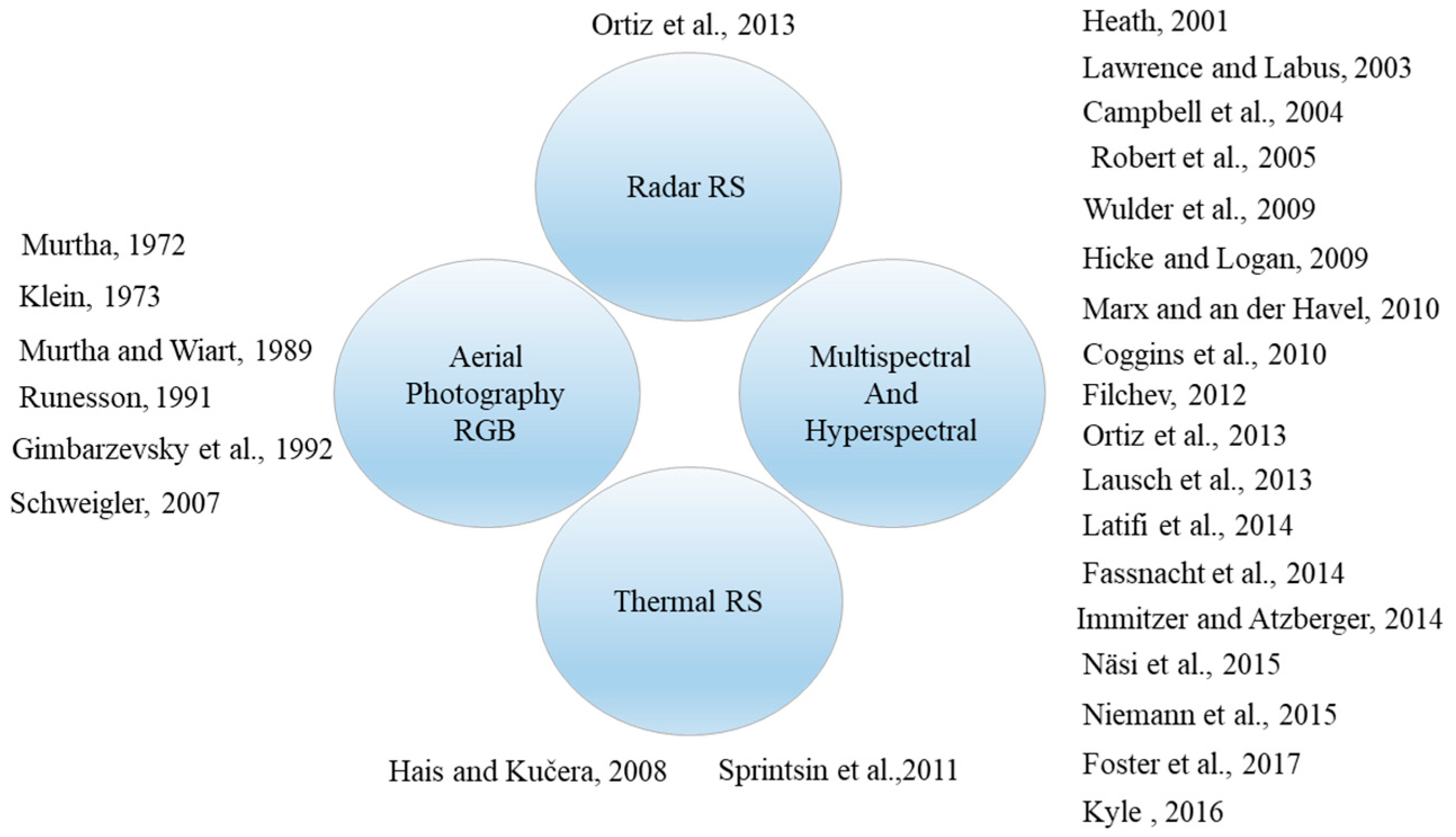
1. Introduction
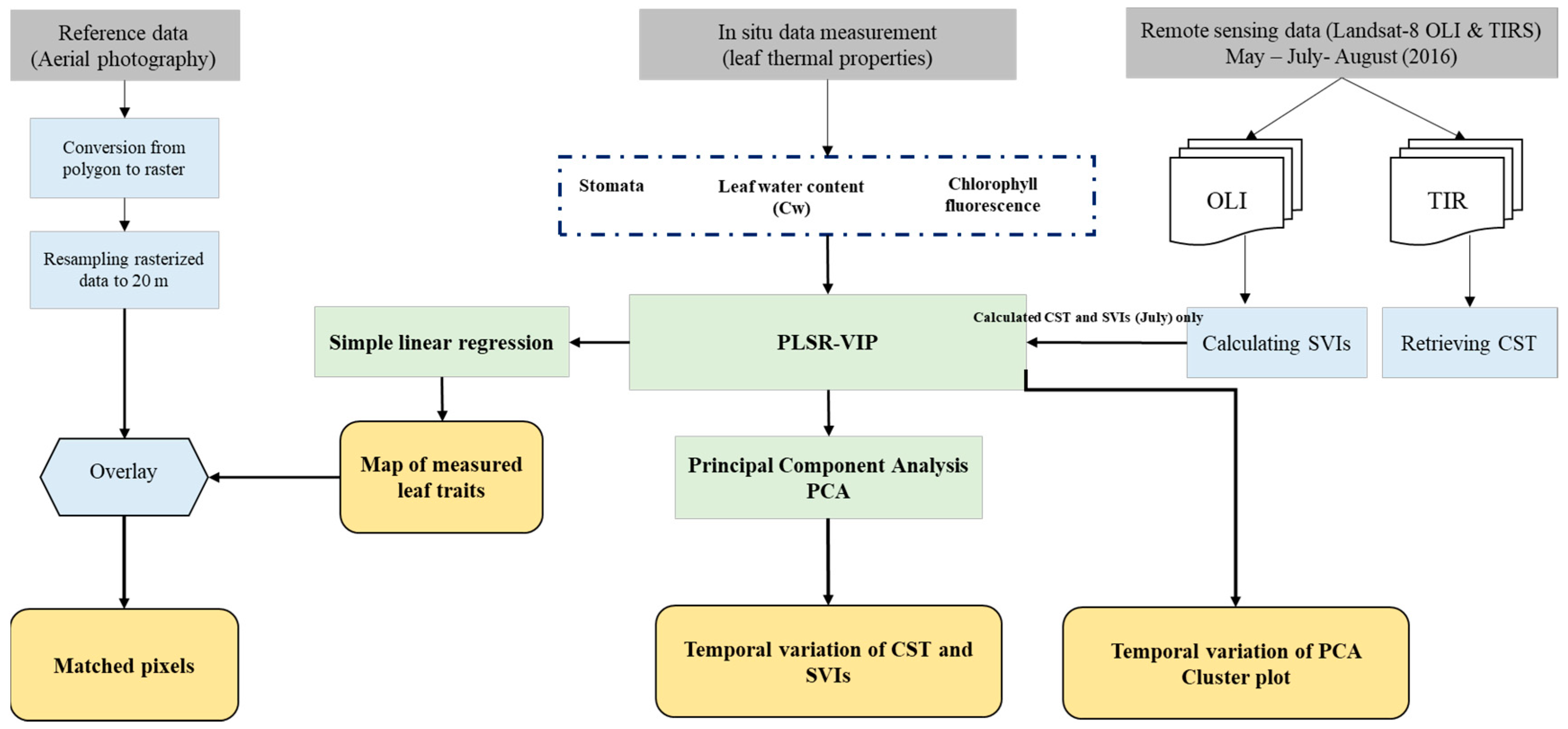
2. Materials and Methods
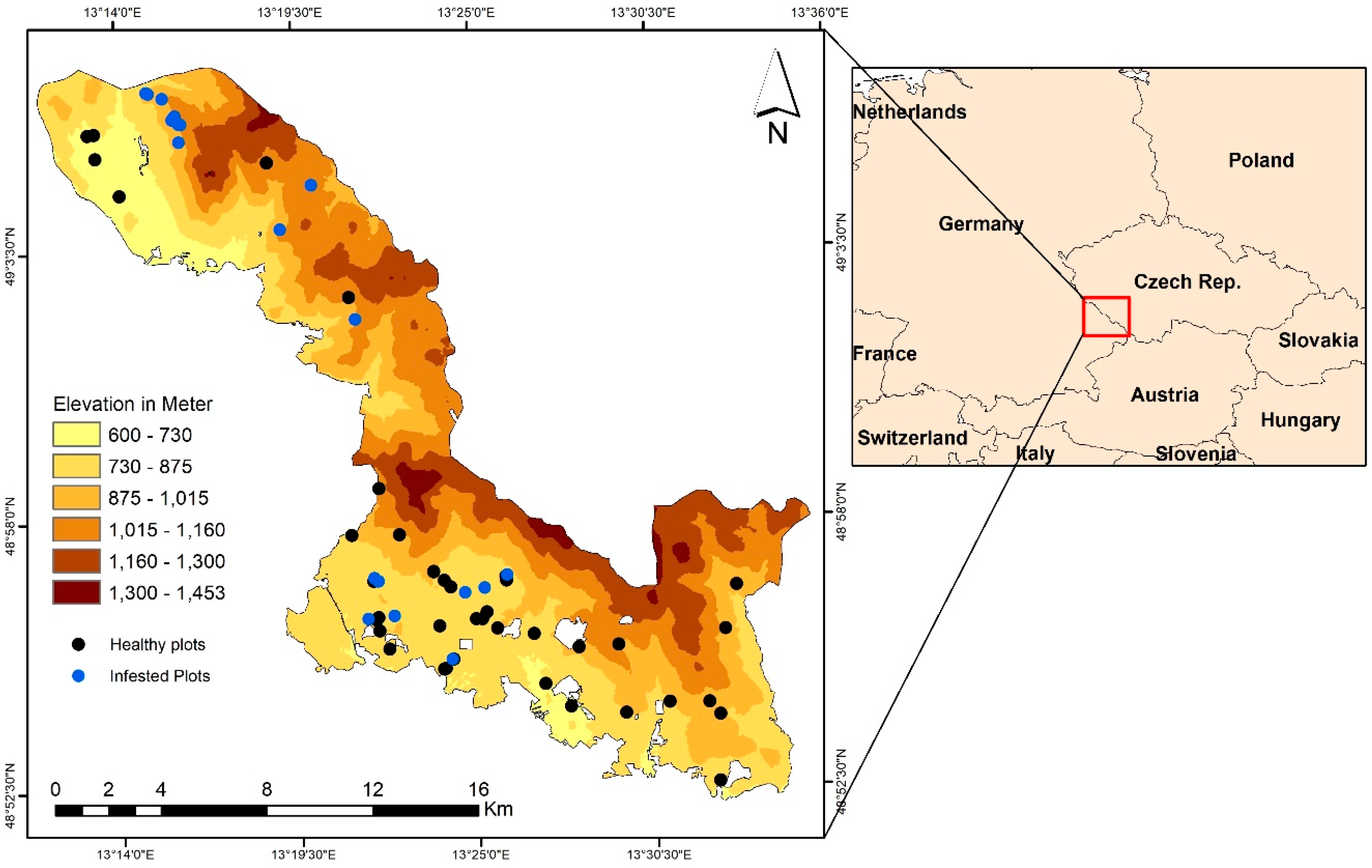
2.1. Study Site and In Situ Data Collection
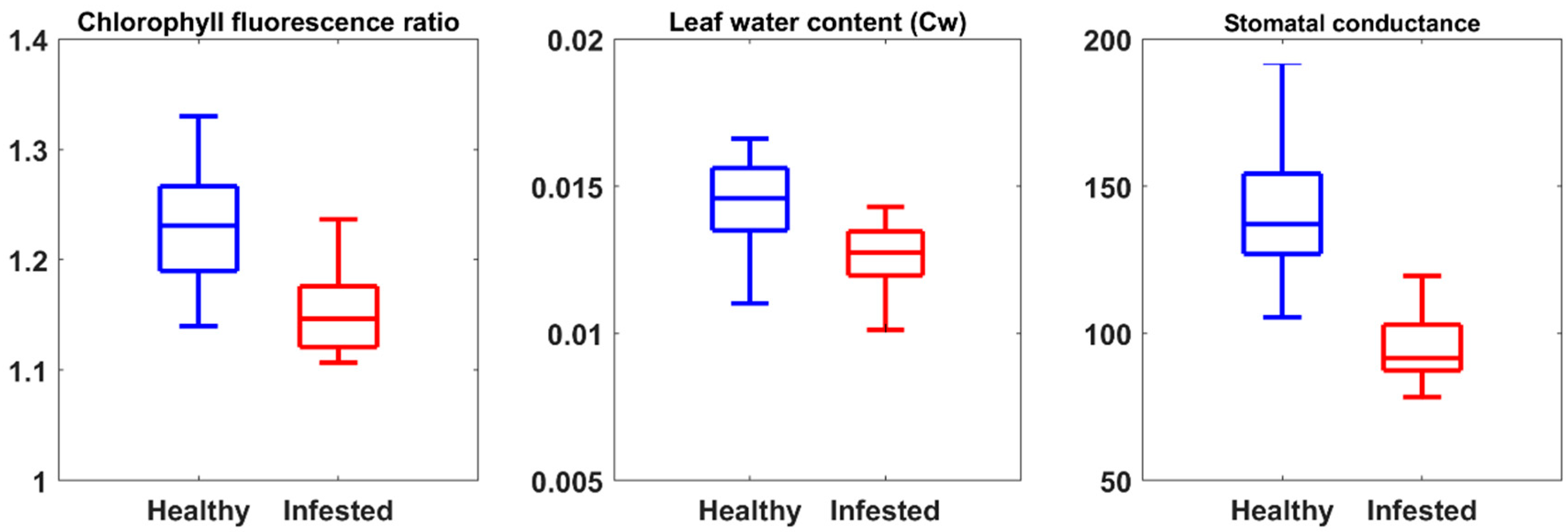
2.2. Measurement of Leaf Properties
2.3. Landsat-8 Imagery and Pre-Processing
2.3.1. Spectral Vegetation Indices
2.3.2. Canopy Surface Temperature (CST)
2.4. Statistical Analysis
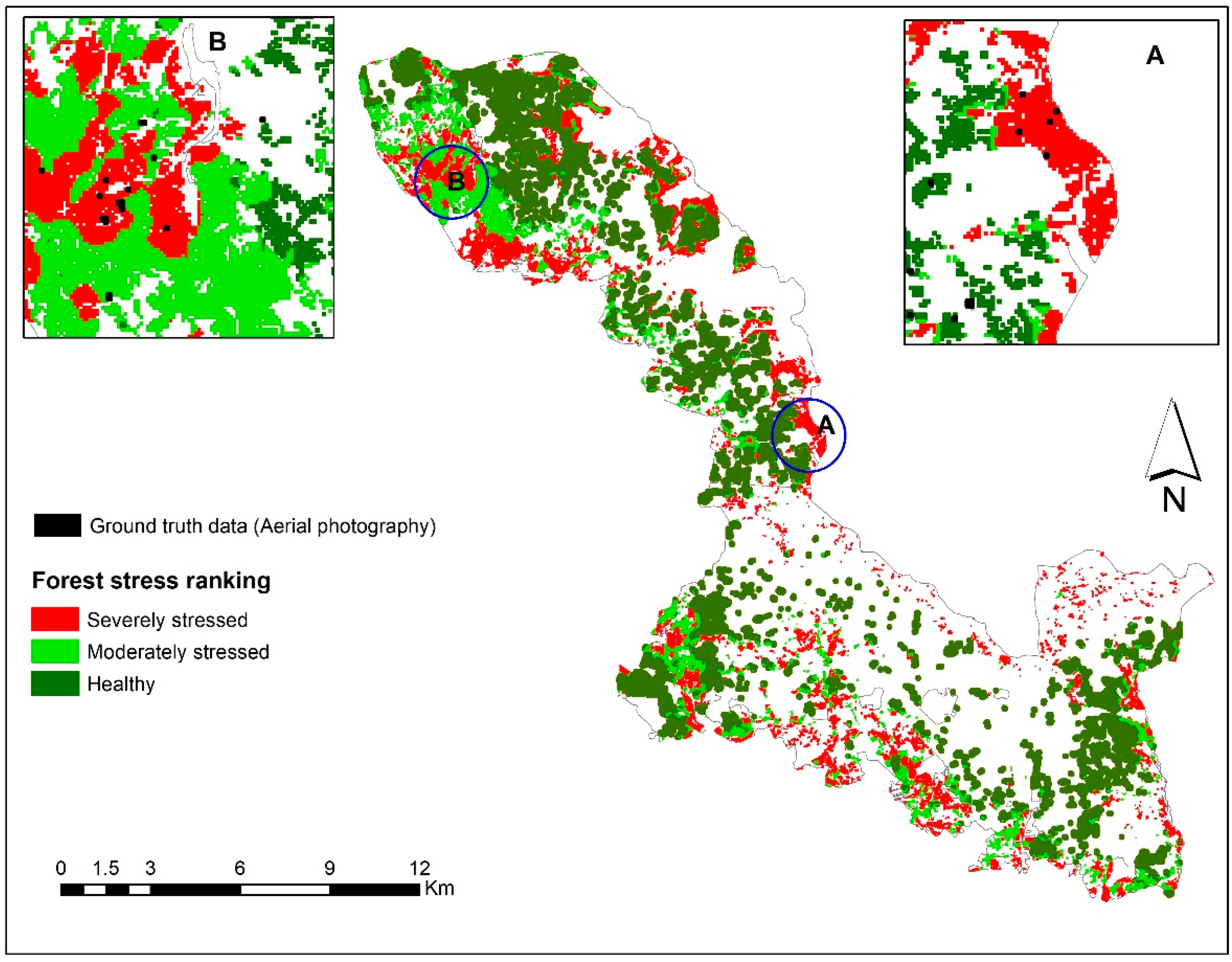
2.5. Mapping Bark Beetle Green Attack Infestation
3. Results
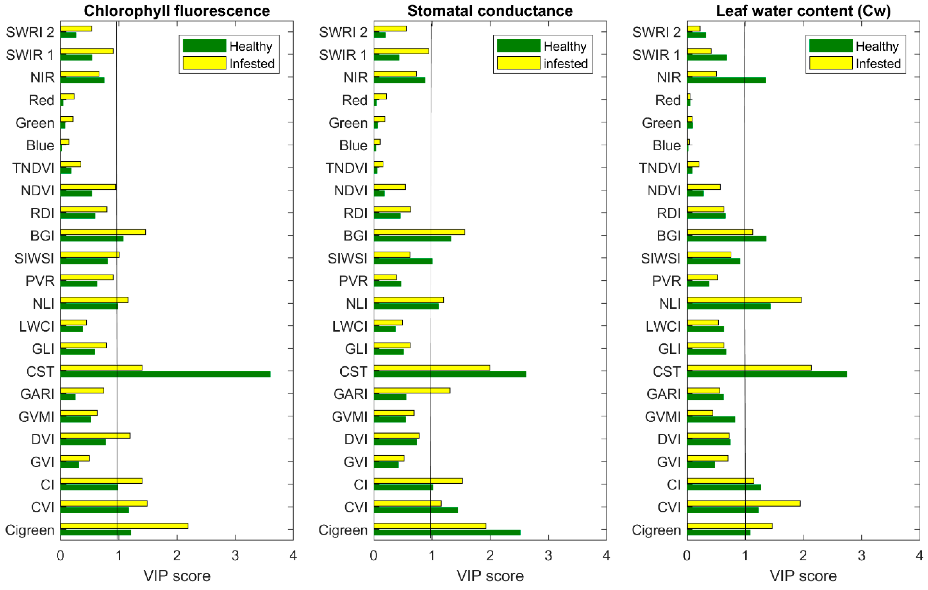
3.1. The Importance of CST versus SVIs to Estimate Measured Leaf Properties
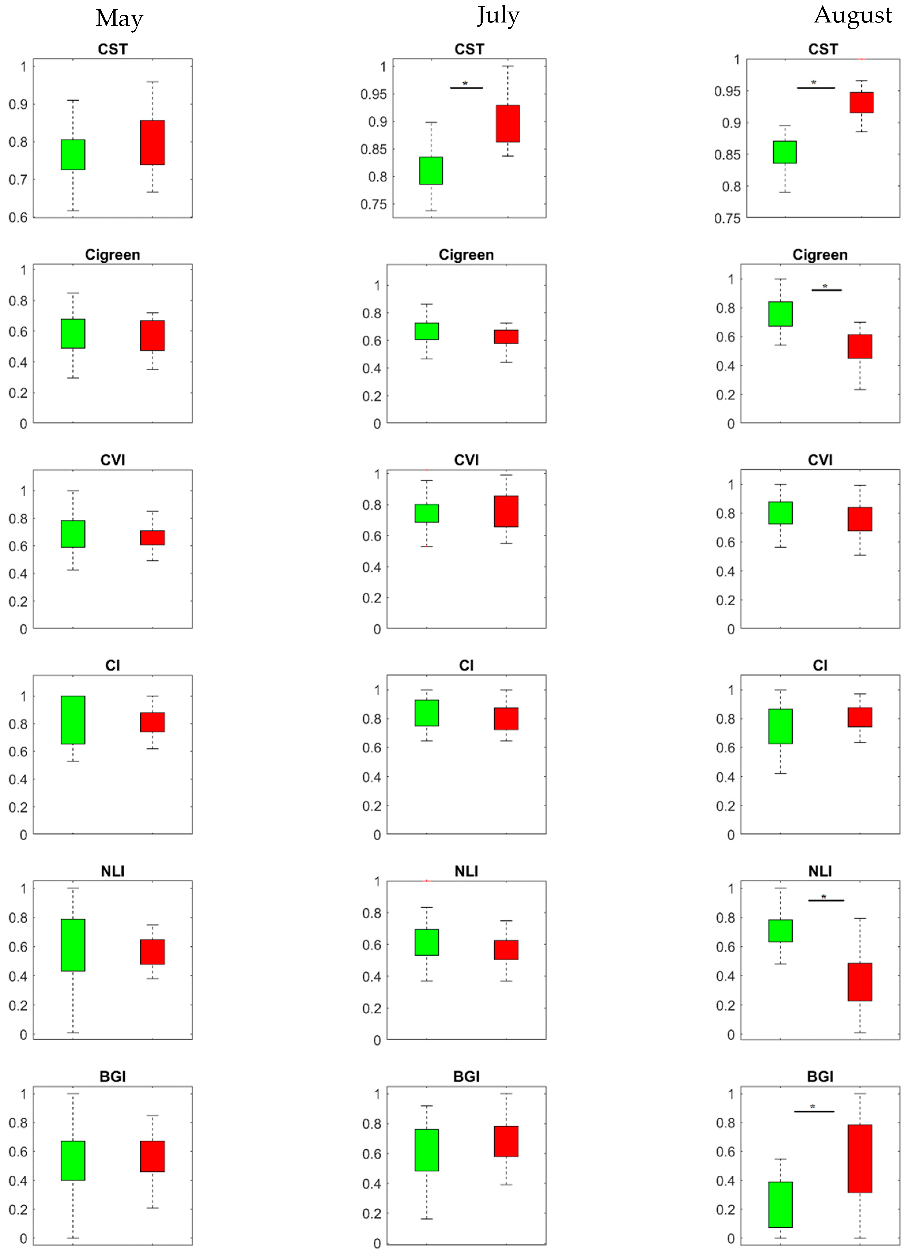
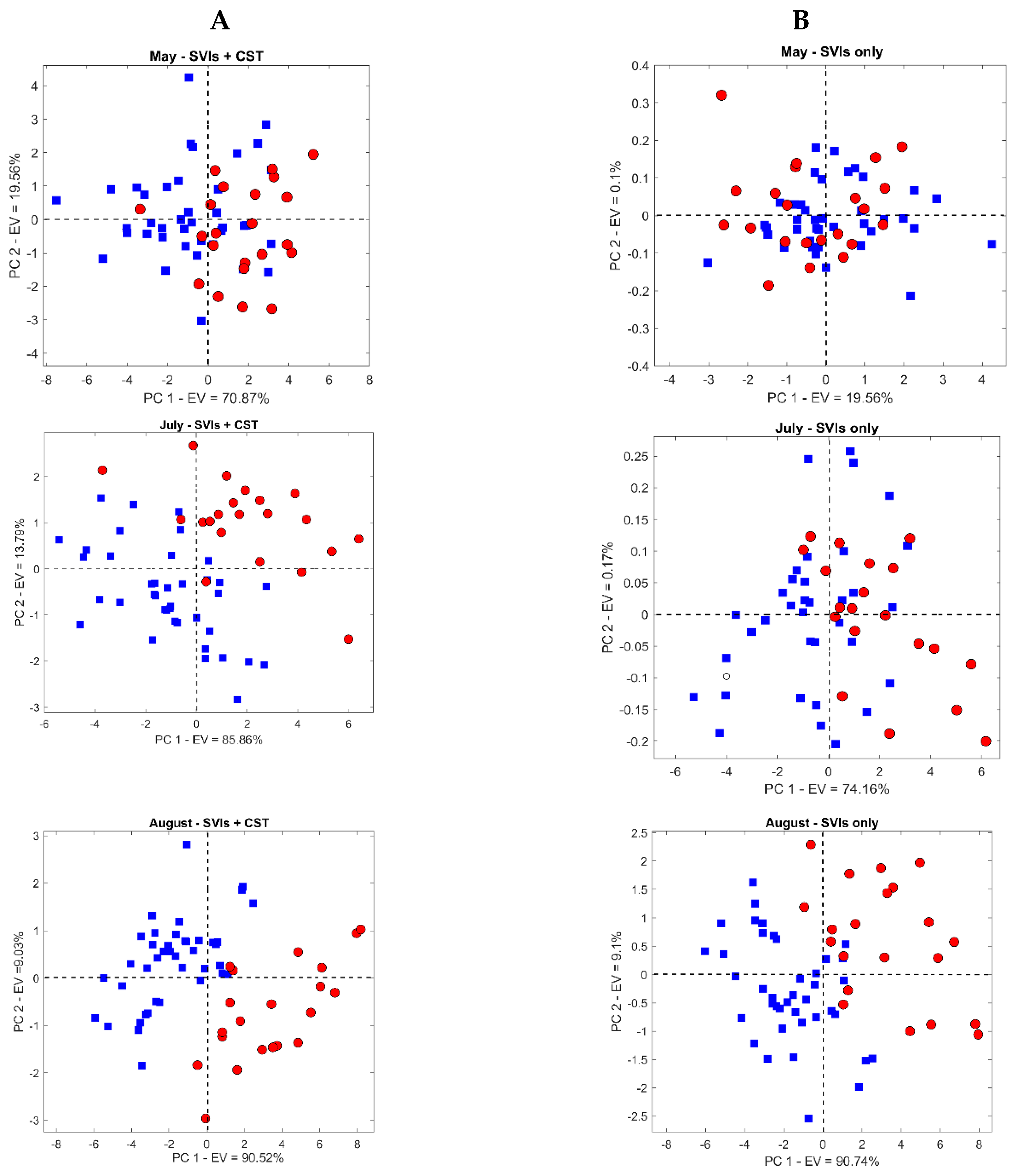
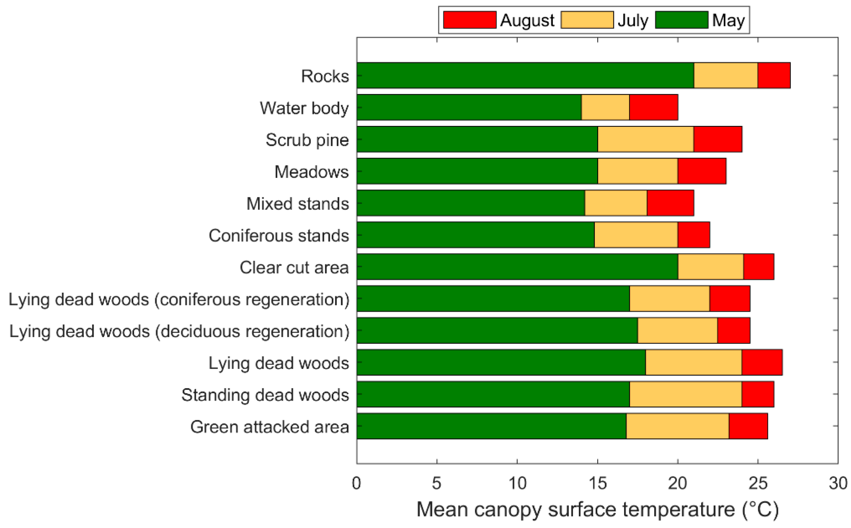
3.2. Temporal Response of CST and SVIs under Spruce Bark Beetle Infestation
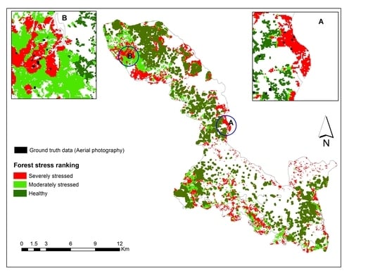
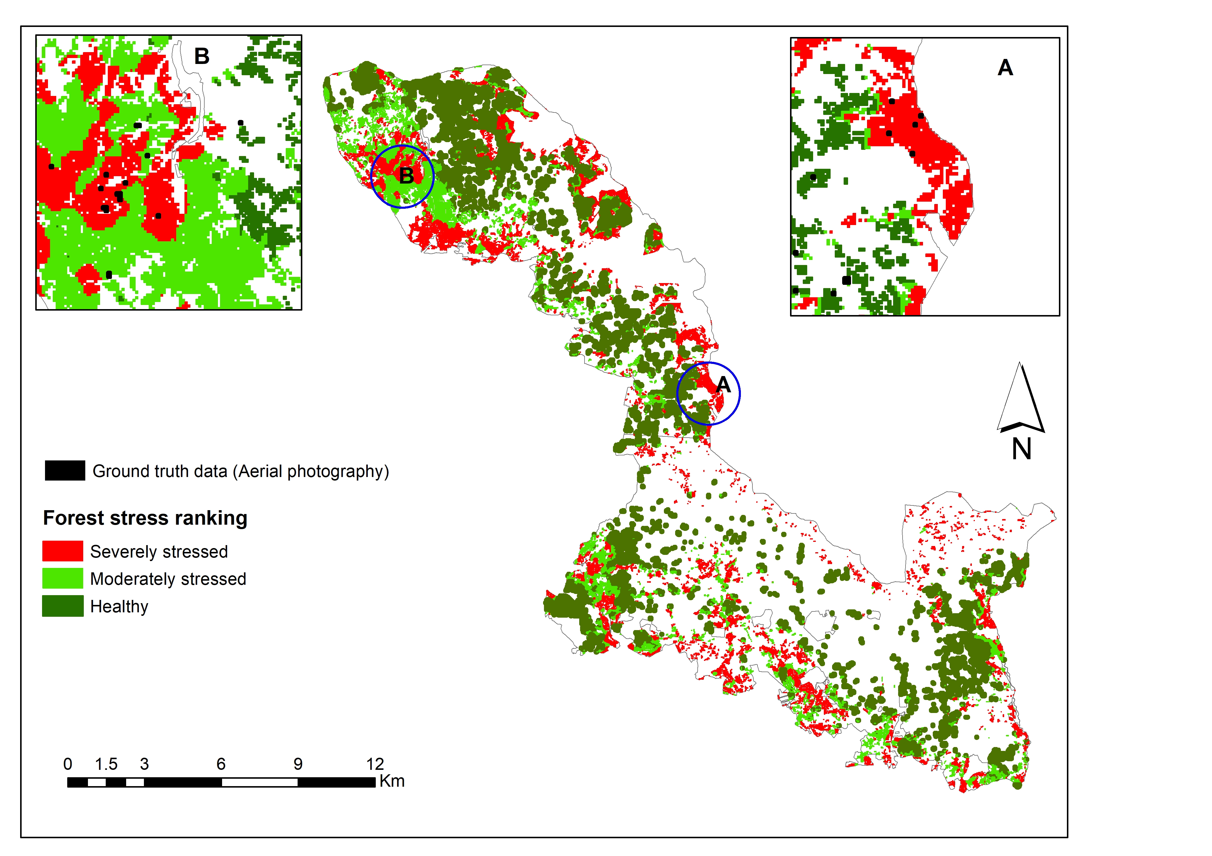
3.3. Mapping Bark Beetle Green Attack and Validation
4. Discussion
5. Conclusions
Author Contributions
Funding
Acknowledgments
Conflicts of Interest
References
- Morris, J.L.; Cottrell, S.; Fettig, C.J.; Hansen, W.D.; Sherriff, R.L.; Carter, V.A.; Clear, J.L.; Clement, J.; DeRose, R.J.; Hicke, J.A.; et al. Managing bark beetle impacts on ecosystems and society: Priority questions to motivate future research. J. Appl. Ecol. 2017, 54, 750–760. [Google Scholar] [CrossRef]
- Tchakerian, M.D.; Coulson, R.N. Ecological Impacts of Southern Pine Beetle; Coulson, R.N., Klepzig, K.D., Eds.; Southern Pine Beetle II. Gen. Tech. Rep. SRS-140; US Department of Agriculture Forest Service, Southern Research Station: Asheville, NC, USA, 2011; Volume 140, pp. 223–234.
- Schelhaas, M.J.; Nabuurs, G.J.; Schuck, A. Natural disturbances in the european forests in the 19th and 20th centuries. Glob. Chang. Biol. 2003, 9, 1620–1633. [Google Scholar] [CrossRef]
- Eidmann, H. Impact of bark beetles on forests and forestry in sweden. J. Appl. Entomol. 1992, 114, 193–200. [Google Scholar] [CrossRef]
- Pasztor, F.; Matulla, C.; Rammer, W.; Lexer, M.J. Drivers of the bark beetle disturbance regime in alpine forests in austria. For. Ecol. Manag. 2014, 318, 349–358. [Google Scholar] [CrossRef]
- Seidl, R.; Rammer, W.; Jäger, D.; Lexer, M.J. Impact of bark beetle (ips typographus l.) disturbance on timber production and carbon sequestration in different management strategies under climate change. For. Ecol. Manag. 2008, 256, 209–220. [Google Scholar] [CrossRef]
- Lehnert, L.W.; Bässler, C.; Brandl, R.; Burton, P.J.; Müller, J. Conservation value of forests attacked by bark beetles: Highest number of indicator species is found in early successional stages. J. Nat. Conserv. 2013, 21, 97–104. [Google Scholar] [CrossRef]
- Müller, J.; Bütler, R. A review of habitat thresholds for dead wood: A baseline for management recommendations in european forests. Eur. J. For. Res. 2010, 129, 981–992. [Google Scholar] [CrossRef]
- Wermelinger, B. Ecology and management of the spruce bark beetle ips typographus—A review of recent research. For. Ecol. Manag. 2004, 202, 67–82. [Google Scholar] [CrossRef]
- Raffa, K.F.; Grégoire, J.-C.; Staffan Lindgren, B. Chapter 1—natural history and ecology of bark beetles. In Bark Beetles; Vega, F.E., Hofstetter, R.W., Eds.; Academic Press: San Diego, CA, USA, 2015; pp. 1–40. [Google Scholar]
- Niemann, K.O.; Visintini, F. Assessment of Potential for Remote Sensing Detection of Bark Beetle-Infested Areas during Green Attack: A Literature Review; Natural Resources Canada, Canadian Forest Service, Pacific Forestry Centre: Victoria, BC, Canada, 2005.
- Wulder, M.A.; White, J.C.; Bentz, B.; Alvarez, M.F.; Coops, N.C. Estimating the probability of mountain pine beetle red-attack damage. Remote Sens. Environ. 2006, 101, 150–166. [Google Scholar] [CrossRef]
- Coulson, R.N.; Amman, G.D.; Dahlsten, D.L.; DeMars, C., Jr.; Stephen, F. Forest-bark beetle interactions: Bark beetle population dynamics. In Integrated Pest Management in Pine-Bark Beetle Ecosystems; John Wiley & Sons: New York, NY, USA, 1985; pp. 61–80. [Google Scholar]
- Wulder, M.A.; Dymond, C.C.; White, J.C.; Leckie, D.G.; Carroll, A.L. Surveying mountain pine beetle damage of forests: A review of remote sensing opportunities. For. Ecol. Manag. 2006, 221, 27–41. [Google Scholar] [CrossRef]
- Filchev, L. An Assessment of European Spruce Bark Beetle Infestation Using WorldView-2 Satellite Data. In Proceedings of the 1st European SCGIS Conference with International Participation Best Practices: Application of GIS Technologies for Conservation of Natural and Cultural Heritage Sites‖ (SCGIS-Bulgaria, Sofia), Sofia, Bulgaria, 21–23 May 2012; pp. 9–16. [Google Scholar]
- Franklin, S.E.; Wulder, M.A.; Skakun, R.S.; Carroll, A.L. Mountain pine beetle red-attack forest damage classification using stratified landsat tm data in british columbia, canada. Photogramm. Eng. Remote Sens. 2003, 69, 283–288. [Google Scholar] [CrossRef]
- Hais, M.; Jonášová, M.; Langhammer, J.; Kučera, T. Comparison of two types of forest disturbance using multitemporal landsat tm/etm+ imagery and field vegetation data. Remote Sens. Environ. 2009, 113, 835–845. [Google Scholar] [CrossRef]
- Havašová, M.; Bucha, T.; Ferenčík, J.; Jakuš, R. Applicability of a vegetation indices-based method to map bark beetle outbreaks in the high tatra mountains. Ann. For. Res. 2015, 58, 295–310. [Google Scholar] [CrossRef]
- Meddens, A.J.H.; Hicke, J.A.; Vierling, L.A.; Hudak, A.T. Evaluating methods to detect bark beetle-caused tree mortality using single-date and multi-date landsat imagery. Remote Sens. Environ. 2013, 132, 49–58. [Google Scholar] [CrossRef]
- Wulder, M.A.; White, J.C.; Carroll, A.L.; Coops, N.C. Challenges for the operational detection of mountain pine beetle green attack with remote sensing. For. Chron. 2009, 85, 32–38. [Google Scholar] [CrossRef]
- Yamaoka, Y.; Swanson, R.; Hiratsuka, Y. Inoculation of lodgepole pine with four blue-stain fungi associated with mountain pine beetle, monitored by a heat pulse velocity (hpv) instrument. Can. J. For. Res. 1990, 20, 31–36. [Google Scholar] [CrossRef]
- Cheng, T.; Rivard, B.; Sánchez-Azofeifa, G.A.; Feng, J.; Calvo-Polanco, M. Continuous wavelet analysis for the detection of green attack damage due to mountain pine beetle infestation. Remote Sens. Environ. 2010, 114, 899–910. [Google Scholar] [CrossRef]
- Buitrago Acevedo, M.F.; Groen, T.A.; Hecker, C.A.; Skidmore, A.K. Identifying leaf traits that signal stress in tir spectra. ISPRS J. Photogramm. Remote Sens. 2017, 125, 132–145. [Google Scholar] [CrossRef]
- Berni, J.A.J.; Zarco-Tejada, P.J.; Gonzalez-Dugo, V.; Fereres, E. Remote sensing of thermal water stress indicators in peach. Acta Hortic. 2012, 962, 325–331. [Google Scholar] [CrossRef]
- Jang, J.D.; Viau, A.A.; Anctil, F. Thermal-water stress index from satellite images. Int. J. Remote Sens. 2006, 27, 1619–1639. [Google Scholar] [CrossRef]
- Sepulcre-Cantó, G.; Zarco-Tejada, P.J.; Jiménez-Muñoz, J.; Sobrino, J.; De Miguel, E.; Villalobos, F.J. Detection of water stress in an olive orchard with thermal remote sensing imagery. Agric. For. Meteorol. 2006, 136, 31–44. [Google Scholar] [CrossRef]
- Hais, M.; Kučera, T. Surface temperature change of spruce forest as a result of bark beetle attack: Remote sensing and gis approach. Eur. J. For. Res. 2008, 127, 327–336. [Google Scholar] [CrossRef]
- Sprintsin, M.; Chen, J.M.; Czurylowicz, P. Combining land surface temperature and shortwave infrared reflectance for early detection of mountain pine beetle infestations in western canada. J. Appl. Remote Sens. 2011, 5, 053566. [Google Scholar] [CrossRef]
- Ullah, S.; Skidmore, A.K.; Ramoelo, A.; Groen, T.A.; Naeem, M.; Ali, A. Retrieval of leaf water content spanning the visible to thermal infrared spectra. ISPRS J. Photogramm. Remote Sens. 2014, 93, 56–64. [Google Scholar] [CrossRef]
- Buitrago, M.F.; Groen, T.A.; Hecker, C.A.; Skidmore, A.K. Changes in thermal infrared spectra of plants caused by temperature and water stress. ISPRS J. Photogramm. Remote Sens. 2016, 111, 22–31. [Google Scholar] [CrossRef]
- Neinavaz, E.; Darvishzadeh, R.; Skidmore, A.K.; Groen, T.A. Measuring the response of canopy emissivity spectra to leaf area index variation using thermal hyperspectral data. Int. J. Appl. Earth Obs. Geoinf. 2016, 53, 40–47. [Google Scholar] [CrossRef]
- Kümmerlen, B.; Dauwe, S.; Schmundt, D.; Schurr, U. Thermography to measure water relations of plant leaves. In Handbook of Computer Vision and Applications; Academic Press: London, UK, 1999; Volume 3, pp. 763–781. [Google Scholar]
- Fabre, S.; Lesaignoux, A.; Olioso, A.; Briottet, X. Influence of water content on spectral reflectance of leaves in the 3–15µm domain. IEEE Geosci. Remote Sens. Lett. 2011, 8, 143–147. [Google Scholar] [CrossRef]
- Xu, H.; Zhu, S.; Ying, Y.; Jiang, H. Early detection of plant disease using infrared thermal imaging. Opt. Nat. Resour. Agric. Foods. 2006, 6381, 638110. [Google Scholar] [CrossRef]
- Oerke, E.; Steiner, U.; Dehne, H.; Lindenthal, M. Thermal imaging of cucumber leaves affected by downy mildew and environmental conditions. J. Exp. Bot. 2006, 57, 2121–2132. [Google Scholar] [CrossRef]
- Ni, Z.; Liu, Z.; Huo, H.; Li, Z.-L.; Nerry, F.; Wang, Q.; Li, X. Early water stress detection using leaf-level measurements of chlorophyll fluorescence and temperature data. Remote Sens. 2015, 7, 3232–3249. [Google Scholar] [CrossRef]
- Aldea, M.; Hamilton, J.G.; Resti, J.P.; Zangerl, A.R.; Berenbaum, M.R. Indirect effects of insect herbivory on leaf gas exchange in soybean. Plant Cell Environ. 2005, 28, 402–411. [Google Scholar] [CrossRef]
- Moller, M.; Alchanatis, V.; Cohen, Y.; Meron, M.; Tsipris, J.; Naor, A.; Ostrovsky, V.; Sprintsin, M.; Cohen, S. Use of thermal and visible imagery for estimating crop water status of irrigated grapevine. J. Exp. Bot. 2007, 58, 827–838. [Google Scholar] [CrossRef] [PubMed]
- Hunt, E.R.; Rock, B.N. Detection of changes in leaf water content using near-and middle-infrared reflectances. Remote Sens. Environ. 1989, 30, 43–54. [Google Scholar]
- Kim, Y.; Still, C.J.; Hanson, C.V.; Kwon, H.; Greer, B.T.; Law, B.E. Canopy skin temperature variations in relation to climate, soil temperature, and carbon flux at a ponderosa pine forest in central oregon. Agric. For. Meteorol. 2016, 226–227, 161–173. [Google Scholar] [CrossRef]
- Gersony, J.T.; Prager, C.M.; Boelman, N.T.; Eitel, J.U.H.; Gough, L.; Greaves, H.E.; Griffin, K.L.; Magney, T.S.; Sweet, S.K.; Vierling, L.A.; et al. Scaling thermal properties from the leaf to the canopy in the alaskan arctic tundra. Arct. Antarct. Alp. Res. 2016, 48, 739–754. [Google Scholar] [CrossRef]
- Doughty, C.E.; Field, C.B.; McMillan, A.M. Can crop albedo be increased through the modification of leaf trichomes, and could this cool regional climate? Clim. Chang. 2011, 104, 379–387. [Google Scholar] [CrossRef]
- Stoner, W.A.; Miller, P.C. Water relations of plant species in the wet coastal tundra at barrow, alaska. Arct. Alp. Res. 1975, 109–124. [Google Scholar] [CrossRef]
- Vanderhoof, M.; Williams, C.A.; Ghimire, B.; Rogan, J. Impact of mountain pine beetle outbreaks on forest albedo and radiative forcing, as derived from moderate resolution imaging spectroradiometer, rocky mountains, USA. J. Geophys. Res. Biogeosci. 2013, 118, 1461–1471. [Google Scholar] [CrossRef]
- Schulze, E.-D.; Hall, A. Stomatal responses, water loss and CO2 assimilation rates of plants in contrasting environments. In Physiological Plant Ecology II; Springer: Berlin, Gremany, 1982; pp. 181–230. [Google Scholar]
- Pierce, L.L.; Congalton, R.G. A methodology for mapping forest latent heat flux densities using remote sensing. Remote Sens. Environ. 1988, 24, 405–418. [Google Scholar] [CrossRef]
- Pierce, L.L.; Running, S.W.; Riggs, G.A. Remote detection of canopy water stress in coniferous forests using the ns001 thematic mapper simulator and the thermal infrared multispectral scanner. PE&RS Photogramm. Eng. Remote Sens. 1990, 56, 579–586. [Google Scholar]
- Méthy, M.; Olioso, A.; Trabaud, L. Chlorophyll fluorescence as a tool for management of plant resources. Remote Sens. Environ. 1994, 47, 2–9. [Google Scholar] [CrossRef]
- Porcar-Castell, A.; Tyystjärvi, E.; Atherton, J.; van der Tol, C.; Flexas, J.; Pfündel, E.E.; Moreno, J.; Frankenberg, C.; Berry, J.A. Linking chlorophyll a fluorescence to photosynthesis for remote sensing applications: Mechanisms and challenges. J. Exp. Bot. 2014, 65, 4065–4095. [Google Scholar] [CrossRef] [PubMed]
- McFarlane, J.; Watson, R.D.; Theisen, A.F.; Jackson, R.D.; Ehrler, W.; Pinter, P.; Idso, S.B.; Reginato, R. Plant stress detection by remote measurement of fluorescence. Appl. Opt. 1980, 19, 3287–3289. [Google Scholar] [CrossRef] [PubMed]
- Campbell, P.; Middleton, E.; McMurtrey, J.; Chappelle, E. Assessment of vegetation stress using reflectance or fluorescence measurements. J. Environ. Qual. 2007, 36, 832–845. [Google Scholar] [CrossRef] [PubMed]
- Heurich, M.; Beudert, B.; Rall, H.; Křenová, Z. National parks as model regions for interdisciplinary long-term ecological research: The bavarian forest and šumavá national parks underway to transboundary ecosystem research. In Long-Term Ecological Research; Springer: Berlin/Heidelberg, Germany, 2010; pp. 327–344. [Google Scholar]
- Bässler, C.; Förster, B.; Moning, C.; Müller, J. The bioklim-project: Biodiversity research between climate change and wilding in a temperate montane forest—The conceptual framework. Waldökologie Landschaftsforschung und Naturschutz 2008, 7, 21–33. [Google Scholar]
- Cailleret, M.; Heurich, M.; Bugmann, H. Reduction in browsing intensity may not compensate climate change effects on tree species composition in the bavarian forest national park. For. Ecol. Manag. 2014, 328, 179–192. [Google Scholar] [CrossRef]
- Ali, A.M.; Darvishzadeh, R.; Skidmore, A.K.; Duren, I.v.; Heiden, U.; Heurich, M. Estimating leaf functional traits by inversion of prospect: Assessing leaf dry matter content and specific leaf area in mixed mountainous forest. Int. J. Appl. Earth Obs. Geoinf. 2016, 45, 66–76. [Google Scholar] [CrossRef]
- Gitelson, A.A.; Buschmann, C.; Lichtenthaler, H.K. The chlorophyll fluorescence ratio f 735/f 700 as an accurate measure of the chlorophyll content in plants. Remote Sens. Environ. 1999, 69, 296–302. [Google Scholar] [CrossRef]
- Waring, R.H. Estimating forest growth and efficiency in relation to canopy leaf area. Adv. Ecol. Res. 1983, 13, 327–354. [Google Scholar]
- Colombo, R.; Meroni, M.; Marchesi, A.; Busetto, L.; Rossini, M.; Giardino, C.; Panigada, C. Estimation of leaf and canopy water content in poplar plantations by means of hyperspectral indices and inverse modeling. Remote Sens. Environ. 2008, 112, 1820–1834. [Google Scholar] [CrossRef]
- Adler-Golden, S.M.; Matthew, M.W.; Bernstein, L.S. Atmospheric correction for Short-wave spectral imagery based on MODTRAN 4[C]. Proc. SPIE 1999, 3753, 61–70. [Google Scholar] [CrossRef]
- FLAASH Module. Atmospheric Correction Module: QUAC and FLAASH User’s Guide; Version 4.7; ITT Visual Information Solutions: Boulder, CO, USA, 2009; p. 44. [Google Scholar]
- Eitel, J.U.; Gessler, P.E.; Smith, A.M.; Robberecht, R. Suitability of existing and novel spectral indices to remotely detect water stress in populus spp. For. Ecol. Manag. 2006, 229, 170–182. [Google Scholar] [CrossRef]
- Abdullah, H.; Skidmore, A.K.; Darvishzadeh, R.; Heurich, M.; Pettorelli, N.; Disney, M. Sentinel-2 accurately maps green-attack stage of european spruce bark beetle (ips typographus, l.) compared with landsat-8. Remote Sens. Ecol. Conserv. 2018. [Google Scholar] [CrossRef]
- Atzberger, C.; Richter, K.; Vuolo, F.; Darvishzadeh, R.; Schlerf, M. Why confining to vegetation indices? Exploiting the potential of improved spectral observations using radiative transfer models. In Proceedings of the Remote Sensing for Agriculture, Ecosystems, and Hydrology XIII, 19–21 September 2011; p. 81740Q. [Google Scholar]
- Malenovsky, Z.; Ufer, C.; Lhotáková, Z.; Clevers, J.G.; Schaepman, M.E.; Albrechtová, J.; Cudlín, P. A new hyperspectral index for chlorophyll estimation of a forest canopy: Area under curve normalised to maximal band depth between 650–725 nm. EARSeL eProc. 2006, 5, 161–172. [Google Scholar]
- Misurec, J.; Kopacková, V.; Lhotáková, Z.; Albrechtova, J.; Hanus, J.; Weyermann, J.; Entcheva-Campbell, P. Utilization of hyperspectral image optical indices to assess the norway spruce forest health status. J. Appl. Remote Sens. 2012, 6, 063545. [Google Scholar]
- Zhang, F.; Zhou, G. Estimation of canopy water content by means of hyperspectral indices based on drought stress gradient experiments of maize in the north plain china. Remote Sens. 2015, 7, 15203–15223. [Google Scholar] [CrossRef]
- Hunt, E.R.; Daughtry, C.; Eitel, J.U.; Long, D.S. Remote sensing leaf chlorophyll content using a visible band index. Agron. J. 2011, 103, 1090–1099. [Google Scholar] [CrossRef]
- Escadafal, R.; Belghit, A.; Ben-Moussa, A. Indices spectraux pour la télédétection de la dégradation des milieux naturels en Tunisie aride. In Proceedings of the Actes du 6ème Symposium international sur les mesures physiques et signatures en télédétection, Val d’Isère, France, 17–24 January 1994; pp. 253–259. [Google Scholar]
- Tucker, C.J.; Elgin Jr, J.H.; McMurtrey Iii, J.; Fan, C. Monitoring corn and soybean crop development with hand-held radiometer spectral data. Remote Sens. Environ. 1979, 8, 237–248. [Google Scholar] [CrossRef]
- Bannari, A.; Morin, D.; Bonn, F.; Huete, A.R. A review of vegetation indices. Remote Sens. Rev. 1995, 13, 95–120. [Google Scholar] [CrossRef]
- Ceccato, P.; Gobron, N.; Flasse, S.; Pinty, B.; Tarantola, S. Designing a spectral index to estimate vegetation water content from remote sensing data: Part 1: Theoretical approach. Remote Sens. Environ. 2002, 82, 188–197. [Google Scholar] [CrossRef]
- Gitelson, A.A.; Kaufman, Y.J.; Merzlyak, M.N. Use of a green channel in remote sensing of global vegetation from eos-modis. Remote Sens. Environ. 1996, 58, 289–298. [Google Scholar] [CrossRef]
- Gobron, N.; Pinty, B.; Verstraete, M.M.; Widlowski, J.-L. Advanced vegetation indices optimized for up-coming sensors: Design, performance, and applications. IEEE Trans. Geosci. Remote Sens. 2000, 38, 2489–2505. [Google Scholar]
- Cohen, W.B. Response of vegetation indices to changes in three measures of leaf water stress. Photogramm. Eng. Remote Sens. 1991, 57, 185–202. [Google Scholar]
- Goel, N.S.; Qin, W. Influences of canopy architecture on relationships between various vegetation indices and lai and fpar: A computer simulation. Remote Sens. Rev. 1994, 10, 309–347. [Google Scholar] [CrossRef]
- Metternicht, G. Vegetation indices derived from high-resolution airborne videography for precision crop management. Int. J. Remote Sens. 2003, 24, 2855–2877. [Google Scholar] [CrossRef]
- Fensholt, R.; Sandholt, I. Derivation of a shortwave infrared water stress index from modis near- and shortwave infrared data in a semiarid environment. Remote Sens. Environ. 2003, 87, 111–121. [Google Scholar] [CrossRef]
- Pinder, J.E.; McLeod, K.W. Indications of relative drought stress in longleaf pine from thematic mapper data. Photogramm. Eng. Remote Sens. 1999, 65, 495–501. [Google Scholar]
- Tucker, C.J. Red and photographic infrared linear combinations for monitoring vegetation. Remote Sens. Environ. 1979, 8, 127–150. [Google Scholar] [CrossRef]
- Bannari, A.; Asalhi, H.; Teillet, P. Transformed difference vegetation index (TDVI) for vegetation cover mapping. In Proceedings of the IEEE International Geoscience and Remote Sensing Symposium (IGARSS ’02), Toronto, ON, Canada, 24–28 June 2002; Volume 5. [Google Scholar]
- Qin, Z.; Karnieli, A.; Berliner, P. A mono-window algorithm for retrieving land surface temperature from landsat tm data and its application to the israel-egypt border region. Int. J. Remote Sens. 2001, 22, 3719–3746. [Google Scholar] [CrossRef]
- Markham, B.L.; Barker, J.L. Landsat MSS and TM Post-Calibration Dynamic Ranges, Exoatmospheric Reflectances and at-Satellite Temperatures. EOSAT Landsat Tech. Notes. 1986, 1, 3–8. [Google Scholar]
- Liu, L.; Zhang, Y. Urban heat island analysis using the landsat tm data and aster data: A case study in hong kong. Remote Sens. 2011, 3, 1535–1552. [Google Scholar] [CrossRef]
- Zhang, J.; Wang, Y.; Li, Y. A c++ program for retrieving land surface temperature from the data of landsat tm/etm+ band6. Comput. Geosci. 2006, 32, 1796–1805. [Google Scholar] [CrossRef]
- Gartland, L. Heat Islands: Understanding and Mitigating Heat in Urban Areas; Earthscan: London, UK, 2008. [Google Scholar]
- Snyder, W.C.; Wan, Z.; Zhang, Y.; Feng, Y.-Z. Classification-based emissivity for land surface temperature measurement from space. Int. J. Remote Sens. 1998, 19, 2753–2774. [Google Scholar] [CrossRef]
- Dozier, J.; Warren, S.G. Effect of viewing angle on the infrared brightness temperature of snow. Water Resour. Res. 1982, 18, 1424–1434. [Google Scholar] [CrossRef]
- Vlassova, L.; Pérez-Cabello, F.; Mimbrero, M.; Llovería, R.; García-Martín, A. Analysis of the relationship between land surface temperature and wildfire severity in a series of landsat images. Remote Sens. 2014, 6, 6136–6162. [Google Scholar] [CrossRef]
- Van de Griend, A.; Owe, M. On the relationship between thermal emissivity and the normalized difference vegetation index for natural surfaces. Int. J. Remote Sens. 1993, 14, 1119–1131. [Google Scholar] [CrossRef]
- Valor, E.; Caselles, V. Mapping land surface emissivity from ndvi: Application to european, african, and south american areas. Remote Sens. Environ. 1996, 57, 167–184. [Google Scholar] [CrossRef]
- Carlson, T.N.; Ripley, D.A. On the relation between ndvi, fractional vegetation cover, and leaf area index. Remote Sens. Environ. 1997, 62, 241–252. [Google Scholar] [CrossRef]
- Sobrino, J.A.; Jiménez-Muñoz, J.C.; Sòria, G.; Romaguera, M.; Guanter, L.; Moreno, J.; Plaza, A.; Martínez, P. Land surface emissivity retrieval from different vnir and tir sensors. IEEE Trans. Geosci. Remote Sens. 2008, 46, 316–327. [Google Scholar] [CrossRef]
- Sun, Q.; Tan, J.; Xu, Y. An erdas image processing method for retrieving lst and describing urban heat evolution: A case study in the pearl river delta region in south china. Environ. Earth Sci. 2010, 59, 1047–1055. [Google Scholar] [CrossRef]
- Farrés, M.; Platikanov, S.; Tsakovski, S.; Tauler, R. Comparison of the variable importance in projection (vip) and of the selectivity ratio (sr) methods for variable selection and interpretation. J. Chemom. 2015, 29, 528–536. [Google Scholar] [CrossRef]
- Wold, S.; Sjöström, M.; Eriksson, L. Pls-regression: A basic tool of chemometrics. Chemom. Intell. Lab. Syst. 2001, 58, 109–130. [Google Scholar] [CrossRef]
- Chong, I.-G.; Jun, C.-H. Performance of some variable selection methods when multicollinearity is present. Chemom. Intell. Lab. Syst. 2005, 78, 103–112. [Google Scholar] [CrossRef]
- Maitra, S.; Yan, J. Principle component analysis and partial least squares: Two dimension reduction techniques for regression. Appl. Multivar. Stat. Models 2008, 79, 79–90. [Google Scholar]
- Lobinger, G. Die lufttemperatur als limitierender faktor für die schwärmaktivität zweier rindenbrütender fichtenborkenkäferarten, lps typographus l. Undpityogenes chalcographus l. (col., scolytidae). Anzeiger für Schädlingskunde 1994, 67, 14–17. [Google Scholar] [CrossRef]
- Abdullah, H.; Darvishzadeh, R.; Skidmore, A.K.; Groen, T.A.; Heurich, M. European spruce bark beetle (ips typographus, l.) green attack affects foliar reflectance and biochemical properties. Int. J. Appl. Earth Obs. Geoinf. 2018, 64, 199–209. [Google Scholar] [CrossRef]
- Ewers, B.; Mackay, D.; Samanta, S. Interannual consistency in canopy stomatal conductance control of leaf water potential across seven tree species. Tree Physiol. 2007, 27, 11–24. [Google Scholar] [CrossRef]
- Chaves, M.M.; Maroco, J.P.; Pereira, J.S. Understanding plant responses to drought—From genes to the whole plant. Funct. Plant Biol. 2003, 30, 239–264. [Google Scholar] [CrossRef]
- Larcher, W. Physiological Plant Ecology: Ecophysiology and Stress Physiology of Functional Groups; Springer Science & Business Media: Berlin/Heidelberg, Germany; Academic Press: New York, NY, USA, 2003. [Google Scholar]
- Fahse, L.; Heurich, M. Simulation and analysis of outbreaks of bark beetle infestations and their management at the stand level. Ecol. Model. 2011, 222, 1833–1846. [Google Scholar] [CrossRef]
- Lausch, A.; Fahse, L.; Heurich, M. Factors affecting the spatio-temporal dispersion of ips typographus (l.) in bavarian forest national park: A long-term quantitative landscape-level analysis. For. Ecol. Manag. 2011, 261, 233–245. [Google Scholar] [CrossRef]
- Dupke, C.; Bonenfant, C.; Reineking, B.; Hable, R.; Zeppenfeld, T.; Ewald, M.; Heurich, M. Habitat selection by a large herbivore at multiple spatial and temporal scales is primarily governed by food resources. Ecography 2017, 40, 1014–1027. [Google Scholar] [CrossRef]
- Peterson, D.L.; Westman, W.E.; Stephenson, N.J.; Ambrosia, V.G.; Brass, J.A.; Spanner, M.A. Analysis of forest structure using thematic mapper simulator data. IEEE Trans. Geosci. Remote Sens. 1986, GE-24, 113–121. [Google Scholar] [CrossRef]
- Junttila, S.; Vastaranta, M.; Hämäläinen, J.; Latva-Käyrä, P.; Holopainen, M.; Hernández Clemente, R.; Hyyppä, H.; Navarro-Cerrillo, R.M. Effect of forest structure and health on the relative surface temperature captured by airborne thermal imagery—Case study in norway spruce-dominated stands in southern finland. Scand. J. For. Res. 2016, 32, 154–165. [Google Scholar] [CrossRef]
- Netherer, S.; Nopp-Mayr, U. Predisposition assessment systems (pas) as supportive tools in forest management—Rating of site and stand-related hazards of bark beetle infestation in the high tatra mountains as an example for system application and verification. For. Ecol. Manag. 2005, 207, 99–107. [Google Scholar] [CrossRef]


| Bands | Wavelength (micrometers) | Resoultion (meters) |
|---|---|---|
| Band-1 (Coastal aerosol) | 0.43–0.45 | 30 |
| Band-2 (Blue) | 0.45–0.51 | 30 |
| Band-3 (Green) | 0.53–0.59 | 30 |
| Band-4 (Red) | 0.64–0.67 | 30 |
| Band-5 (Near Infrared –NIR) | 0.85–0.88 | 30 |
| Band-6 (SWIR-1) | 1.57–1.65 | 30 |
| Band-7 (SWIR-2) | 2.11–2.29 | 30 |
| Band-9 (Panchromatic) | 0.50–0.68 | 15 |
| Band-10 (Cirrus) | 1.36–1.38 | 30 |
| Band-11 (Thermal infrared-TIRS1) | 10.60–11.19 | 100 (resampled to 30) |
| Band-12 (Thermal infrared-TIRS2) | 11.50–12.51 | 100 (resampled to 30) |
| Index | Formula | Full Name | Reference |
|---|---|---|---|
| Cigreen | (NIR/Green) − 1 | Chlorophyll index green | [67] |
| CVI | NIR × (Red/Green2) | Chlorophyll vegetation index | [67] |
| CI | (Red – Blue)/Red | Coloration index | [68] |
| GVI | NIR − Green | Green difference vegetation index | [69] |
| DVI | 2.4 × (NIR – Red) | Difference vegetation index | [70] |
| GVMI | [(NIR + 0.1) − (SWIR +0.02)]/[(NIR + 0.1) + (SWIR + 0.02)] | Global vegetation moisture index | [71] |
| GARI | [NIR − (Green − (Blue − Red))]/[NIR − (Green + (Blue − Red))] | Green atmospherically resistant vegetation index | [72] |
| GLI | [2×(Green − Red − Blue)]/[2 × (Green + Red + Blue)] | Green leaf index | [73] |
| LWCI | [log(1 − (NIR − SWIR))]/[log(1 − (NIR + SWIR))] | Leaf water content index | [74] |
| NLI | (NIR − Red)/( NIR + Red) | Nonlinear vegetation index | [75] |
| PVR | (Green – Red)/(Green + Red) | Normalized Difference Photosynthetic vigour ratio | [76] |
| SIWSI | (NIR-SWIR)/(NIR + SWIR) | Normalized Difference 860/1640 | [77] |
| BGI | Costal/Green | Blue-green pigment index | This study |
| RDI | SWIR2/NIR | Ratio Drought Index | [78] |
| NDVI | (NIR − Red)/(NIR + Red) | Normalized difference vegetation index | [79] |
| TNDVI | Log [(NIR − Red)/NIR + Red) × 0.5] | Transformed NDVI | [80] |
| Severely Stressed | Moderately Stressed | Healthy | |
|---|---|---|---|
| Leaf water content (g/cm2) | <0.0135 | 0.135–0.0145 | >0.0145 |
| Stomatal conductance (mmol/m2s) | <103 | 103–120 | >120 |
| Chlorophyll fluorescence ratio | <1.17 | 1.17–1.25 | >1.25 |
| Equation No. | Regression Equations |
|---|---|
| 1 | Leaf water content = −0.0004 CST + 0.0203 |
| 2 | Stomatal conductance = −6.4377 CST + 255.66 |
| 3 | Chlorophyll fluorescence = −0.0264 CST + 1.68 |
| Forest Stress Classes | Pixels Correctly Matched |
|---|---|
| Severely stressed | 274 |
| Moderately stressed | 89 |
| Healthy | 54 |
© 2019 by the authors. Licensee MDPI, Basel, Switzerland. This article is an open access article distributed under the terms and conditions of the Creative Commons Attribution (CC BY) license (http://creativecommons.org/licenses/by/4.0/).
Share and Cite
Abdullah, H.; Darvishzadeh, R.; Skidmore, A.K.; Heurich, M. Sensitivity of Landsat-8 OLI and TIRS Data to Foliar Properties of Early Stage Bark Beetle (Ips typographus, L.) Infestation. Remote Sens. 2019, 11, 398. https://doi.org/10.3390/rs11040398
Abdullah H, Darvishzadeh R, Skidmore AK, Heurich M. Sensitivity of Landsat-8 OLI and TIRS Data to Foliar Properties of Early Stage Bark Beetle (Ips typographus, L.) Infestation. Remote Sensing. 2019; 11(4):398. https://doi.org/10.3390/rs11040398
Chicago/Turabian StyleAbdullah, Haidi, Roshanak Darvishzadeh, Andrew K. Skidmore, and Marco Heurich. 2019. "Sensitivity of Landsat-8 OLI and TIRS Data to Foliar Properties of Early Stage Bark Beetle (Ips typographus, L.) Infestation" Remote Sensing 11, no. 4: 398. https://doi.org/10.3390/rs11040398
APA StyleAbdullah, H., Darvishzadeh, R., Skidmore, A. K., & Heurich, M. (2019). Sensitivity of Landsat-8 OLI and TIRS Data to Foliar Properties of Early Stage Bark Beetle (Ips typographus, L.) Infestation. Remote Sensing, 11(4), 398. https://doi.org/10.3390/rs11040398