Article

Using Sentinel-2 Multispectral Images to Map the Occurrence of the Cossid Moth (Coryphodema tristis) in Eucalyptus Nitens Plantations of Mpumalanga, South Africa

by
Samuel Takudzwa Kumbula
*,
Paramu Mafongoya
,
Kabir Yunus Peerbhay
,
Romano Trent Lottering
and
Riyad Ismail
School of Agricultural, Earth and Environmental Sciences, University of KwaZulu-Natal, P/Bag X01, Scottsville 3209, Pietermaritzburg, South Africa
*
Author to whom correspondence should be addressed.
Remote Sens. 2019, 11(3), 278; https://doi.org/10.3390/rs11030278
Submission received: 18 September 2018 / Revised: 19 November 2018 / Accepted: 28 November 2018 / Published: 31 January 2019
(This article belongs to the Special Issue Forest Health Monitoring)

Abstract

:
Coryphodema tristis is a wood-boring insect, indigenous to South Africa, that has recently been identified as an emerging pest feeding on Eucalyptus nitens, resulting in extensive damage and economic loss. Eucalyptus plantations contributes over 9% to the total exported manufactured goods of South Africa which contributes significantly to the gross domestic product. Currently, the distribution extent of the Coryphodema tristis is unknown and estimated to infest Eucalyptus nitens compartments from less than 1% to nearly 80%, which is certainly a concern for the forestry sector related to the quantity and quality of yield produced. Therefore, the study sought to model the probability of occurrence of Coryphodema tristis on Eucalyptus nitens plantations in Mpumalanga, South Africa, using data from the Sentinel-2 multispectral instrument (MSI). Traditional field surveys were carried out through mass trapping in all compartments (n = 878) of Eucalyptus nitens plantations. Only 371 Eucalyptus nitens compartments were positively identified as infested and were used to generate the Coryphodema tristis presence data. Presence data and spectral features from the area were analysed using the Maxent algorithm. Model performance was evaluated using the receiver operating characteristics (ROC) curve showing the area under the curve (AUC) and True Skill Statistic (TSS) while the performance of predictors was analysed with the jack-knife. Validation of results were conducted using the test data. Using only the occurrence data and Sentinel-2 bands and derived vegetation indices, the Maxent model provided successful results, exhibiting an area under the curve (AUC) of 0.890. The Photosynthetic vigour ratio, Band 5 (Red edge 1), Band 4 (Red), Green NDVI hyper, Band 3 (Green) and Band 12 (SWIR 2) were identified as the most influential predictor variables. Results of this study suggest that remotely sensed derived vegetation indices from cost-effective platforms could play a crucial role in supporting forest pest management strategies and infestation control.

1. Introduction

In South Africa, emerging forest pests have caused extensive damage to Eucalyptus plantations [1]. Approximately 1.3 million hectares of South African land is composed of both hard and softwoods with the majority located in the eastern parts of the country; primarily in Mpumalanga (40.8%), KwaZulu-Natal (39.5%) and the Eastern Cape (11.1%) [2]. These plantations contribute annually to South Africa’s gross domestic product with Eucalyptus plantations contributing over 9% to the total of exported manufactured goods [3]. These species are the most productive planted exotics that mostly offer timber, pulp and paper in South Africa [4,5,6]. Therefore, a robust mechanism needs to be established to prevent excessive damage, as numerous investments have been injected into the forestry sector, particularly the Mpumalanga province [7]. Since 2004, Coryphodema tristis, commonly known as Cossid moth, has been the major cause of damage to Eucalyptus nitens resources across Mpumalanga, with forest managers requiring up-to-date information to support their forest protection interventions at ground level [8,9,10].
C. tristis is an indigenous wood-boring insect that commonly infests tree families, such as Ulmaceae (Elm Family), Vitaceae (Wild Grape family), Rosaceae (Rose family), Scrophulariaceae (Figwort family), Malvaceae (Mallow family) and Combretaceae (Indian almond family) [11,12]. However, a sudden shift by the C. tristis to infest E. nitens in Southern Africa has been observed. According to Gebeyehu et al. [10], the shift of the C. tristis to infest E. nitens trees may be caused by a few to non-existent natural enemies in the area. As a result, the absence of natural enemies influences the increase of pests in the geographic area, due to less interspecific competition [13]. This results in the moth breeding and multiplying at faster rates and increasing the intensities of E. nitens infestation. Adult female moths lay eggs on the bark of the E. nitens trees and the larvae feed on the bark damaging the cambium [10]. The damage reduces the movement of water within the tree and also extends to the trunk and branches which turn black [8]. Furthermore, as the larvae grow, it drills extensive tunnels into the sapwood and hardwood of the E. nitens which results in the trees producing resin on their trunks and branches and sawdust on the base of the forest floor [11]. However, extensive tunnelling by the moth has resulted in severe damage to trees increasing the probability of tree mortality. Additionally, pupal casings are found protruding on the tunnelled bark or either at the base of the floor indicating the presence of C. tristis.
In recent years, researchers have attempted to use environmental variables to predict the spatial distribution of C. tristis [8,11]. For example, Boreham [9] conducted a study that investigated the outbreak and impact of C. tristis on E. nitens in the Highveld of Mpumalanga, using environmental variables and the Residual Maximum Likelihood (REML) statistical method. The results showed that older E. nitens trees (above 8 years) and lower elevation sites less than 1600 m were the most susceptible to C. tristis infestations. Similarly, Adam et al. [8] used climatic and topographical variables to map the presence and extent of C. tristis infestations in E. nitens plantations of Mpumalanga. Using a random forest classifier, results indicated that with September and April’s maximum temperatures; April’s median rainfall and elevation played a crucial role in identifying conditions that are suitable for C. tristis occurrence. Their results furthermore predicted that areas with a maximum temperature greater than 23 °C in September and 22 °C in April were the most susceptible to infestation. While these studies have successfully utilised environmental and climatic variables to predict the presence of the moth, different studies have identified a number of limitations regarding traditional data collection methods to determine the presence or absence of pests.
Different studies stated that traditional methods such as field surveys are mostly time-consuming, costly, labour-intensive, spatially restrictive and likely unreliable as data collection is based on the knowledge of the surveyor [14,15]. Hence, a direct detection approach that provides real-time information and can be repeated regularly for up-to-date decisions is required. Furthermore, utilizing environmental or climatic variables only for mapping the spatial distribution of pests can be challenging since these variables focus precisely on the surrounding factors and not the actual damage of plantations. For example, Germishuizen et al. [16] utilized environmental factors to determine the susceptibility of pine compartments to bark stripping by Chacma baboons (Papio ursinus). Results indicated that indirect variables such as altitude provide a challenge in explaining the complex relationship of baboon-damage risk. Moreover, Donatelli et al. [17] indicated that observed environmental datasets alone were no longer sufficient to predict the behaviour of pests due to climate change that has influenced the variability of temperature averages, rainfall means and distributions. Thus, requiring more traditional field surveys to confirm whether a particular area has been truly infested. Bouwer et al. [11] indicated that actual confirmation of infestation was certainly confirmed by tree felling which is impossible for large-scale assessments. Hence, the use of remotely sensed data with the ancillary data such as environmental and climatic variables would provide an up-to-date, repeatable source of information for forest assessment and inventory.
Remote sensing has improved the accuracy of predictions of forest-damaging pests using narrow and broad bands in the visible, near, shortwave-infrared and red edge regions [15,18,19]. For example, Adelabu et al. [20] sought to discriminate the levels of change in forest canopy cover instigated by insect defoliation using hyperspectral data in mopane woodland. Results indicated that the overall accuracy of classification was 82.42% using a random forest algorithm and was 81.21% using ANOVA. In another study, Oumar and Mutanga [19] successfully assessed the potential of WorldView-2 bands, environmental variables, as well as vegetation indices which resulted in the prediction of Thaumastocoris peregrinus infestations on Eucalyptus trees. Results indicated that WorldView-2 sensor bands and indices predicted T. peregrinus damage with an R2 value of 0.65 and a root mean square error of 3.62% in an independent test data set. Similarly, Lottering et al. [18] also found that vegetation indices derived from the red edge region correlated with Gonipterus scutellatus-induced vegetation defoliation using WorldView-2 satellite data. Furthermore, Pietrzykowski et al. [15] assessed the presence and severity of defoliation and necrosis caused by the Mycosphaerella fungus in a Eucalyptus globulus plantation, using multi-spectral imagery in north-western Tasmania, Australia. Their results indicated that high spatial resolution airborne digital imagery performed well, producing an accuracy of 71% for defoliation and 67% for necrosis. Therefore, despite the optimal modelling accuracies attained using multispectral remotely sensed data in these studies, these data sets are expensive and limited to a local scale. In this regard, there is an urgent need for testing and assessing the utility of other cheaper data sets that could capture the disease and pest incidences at landscape levels.
This study, therefore, sought to model the probability of the occurrence of the C. tristis on E. nitens plantations in Mpumalanga, South Africa using the cost-effective Sentinel-2 multispectral instrument and derived vegetation indices. Sentinel-2 images across the valuable red edge portion of the electromagnetic spectrum are suitable for forest health applications related to pest and disease damage detection [21,22]. The large swath width and a 5-day temporal resolution make this sensor suitable for repeatable monitoring over forest plantations and detect pest-related damage continuously for effective management and control. Therefore, we used Maxent a robust machine-learning algorithm to predict the probability of the occurrence of the C. tristis using remotely sensed data.

2. Materials and Methods
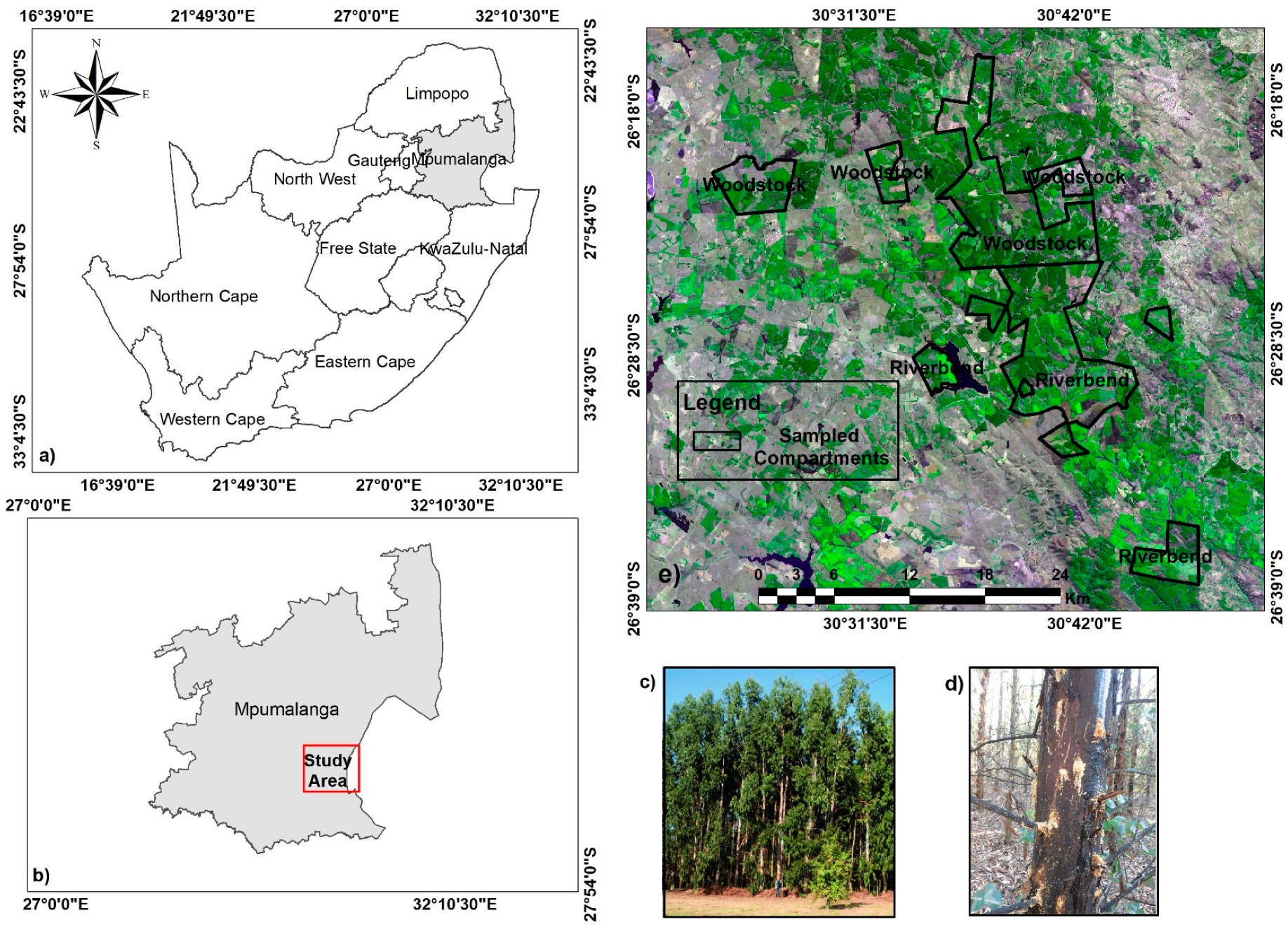
2.1. Study Area

The research was conducted in the Mpumalanga province of South Africa in the Lothair village, also known as Silindile, and is located in the Msukaligwa Local Municipality (Figure 1). The study site is located between 26°26′25.08″ S and 30°3′59.4″ E in the Highveld of Mpumalanga. Elevation of the study area ranges from 1200 to 2100 m above sea level.
The area is associated with between 783–1200 mm of rainfall on average per year from November to March. The Highveld has a summer (October to February) to winter (April to August) temperature range of approximately 19 °C, with average temperatures ranging between 8 °C and 26 °C in the contrasting seasons. The Highveld is among South Africa’s highly productive commercial plantation forests that consist of Pine and Eucalyptus plantations. Greater parts of the Highveld are comprised of sandstone and granite derived soils which the majority of commercial tree species are grown.

2.2. Image Acquisition

A cloud-free Sentinel-2A MSI image of the study area acquired on 19 August 2016, was downloaded from the United States Geological Survey website (www.earthexplorer.ugs.gov). The MSI sensor has a revisit time of 5 days making the detection of pest damage to vegetation instantaneous [21,23,24]. The MSI sensor covers a large area with a swath width of 290 km for increasing the spatial coverage of area of interest [22,24]. Sentinel-2A has thirteen bands ranging from 443.9 nm to 2202.4 nm including four 10 m visible and near-infrared bands, six 20 m red edge, near infrared and shortwave infrared bands and three 60 m bands visible, near-infrared and shortwave infrared bands. The narrow red edge bands cover spectral regions of 703.9 nm, 740.2 nm and 782.5 nm that can be utilised for monitoring vegetation status [22,23,25].

2.3. Image Processing and Analysis

Atmospheric correction of the image was done using the Sentinel Application Platform (SNAP) software, which incorporates the plugin, Sen2Cor. In total, ten bands were derived for modelling the probability of the occurrence of the C. tristis as shown in Table 1. In this study, Sentinel-2A bands 1, 9 and 10 were excluded because of their sensitivity to aerosol, clouds and spatial resolution (60 m). Furthermore, these three bands are not used for vegetation mapping.
Using the Index Database (https://www.indexdatabase.de/db/i.php), we selected vegetation indices with the best capacity to detect and map the occurrence of the C. tristis (see Table 2). Additionally, a number of published vegetation indices that have been effective in characterizing vegetation defoliation, many of which are sensitive to reflectance in the visible and NIR regions were derived. However, vegetation indices with wavelengths from the red edge region were given more emphasis based on their ability to identify stressed vegetation [18].

2.4. Field Data Collection

On the 19 August 2016, a field visit was conducted in two South African Pulp and Paper Industries (SAPPI) plantations totalling 23,928 hectares to establish the presence/absence of the pest in the area. SAPPI plantations are divided into two blocks namely, Woodstock and Riverbend that contains 878 E. nitens compartments. Compartments are partitioned from the blocks that contain the E. nitens plantations and vary in size. Woodstock is located in the northern region of the SAPPI plantation and consists of 55 E. nitens plantations, whilst Riverbend located in the southern region comprises of 1145 plantations. Field crews from SAPPI were assigned different compartments to assist with field work in order to cover the whole study area. To determine the presence/absence of the C. tristis in E. nitens compartments, we used a quadrat sampling technique to carry out mass trapping of C. tristis. Mass trapping was carried out from 15 June to 19 August 2016 using a minimum of 19 and a maximum of 348 yellow bucket funnel traps with pheromone lures across all E. nitens compartments. Pheromones that match the chemical scent of a female adult moth was used to lure male moths into the traps that were located in the compartments [8]. The number of traps used in the field varied with the size of the compartments where traps were placed at 50 m apart from each other hence, in bigger compartments there were more traps compared to smaller compartments. To determine the presence/absence, the sawdust and resin on the stem or the base of the tree were used as indicators of the presence/absence of the C. tristis. Locations of these indicators were then measured using a handheld Trimble GeoHX 6000 Global Positioning System (GPS) with a sub-meter accuracy (<10 cm). The dataset of pest damage indicators was then used to extract spectra from the Sentinel-2A image and develop training and testing datasets for statistical analysis.

2.5. Maxent Modelling Approach

The freely available Maxent approach (version 3.4.0) is developed for species distribution modelling (SDM) and was used in this study for modelling the probability of the occurrence of the C. tristis (http://biodiversityinformatics.amnh.org/open_source/maxent/) [35]. Maxent is a machine learning technique that uses presence-only data to determine the potential spatial suitability preference of species [35,36]. The model evaluates the probability of the occurrence from a number of spatial environmental variables [37,38,39]. For Maxent to determine the probability of occurrence and reduce uncertainty, it requires more presence information of the target species [40]. The background dataset definition contributes to the model’s output significantly and requires the species full environmental distribution of those areas that have been searched [41]. As a result, Maxent establishes a model with a maximum entropy in relation to the data of presence locations and variables to similar interactions with background locations [36,41].
In this study, a total of 20 predictor variables with a correlation −0.8 < r < 0.8 were considered for determining the probability of the occurrence of C. tristis. Bands and vegetation indices from Sentinel-2A MSI data were used to run four model scenarios in Maxent to determine the probability of the occurrence of the C. tristis (as shown in Table 3). These four model scenarios were carried out independently to identify which predictor variables were more robust in modelling the probability of the occurrence of the C. tristis.

2.6. Model Accuracy Assessment

For this study, presence data of the C. tristis infested locations (n = 371) within the compartments were randomly partitioned into two sets, 70% training data (n = 259) and 30% test data (n = 111). A sub-sample was used as the replicate run and iterations were fixed to 500. The regularization multiplier was maintained at 4 to avoid overfitting of the test data [36]. The remaining model values were set to default values. A complementary log-log (clog log) output was utilised because it strongly predicts areas of moderately high output compared to the logistic output [34]. To avoid bias of estimation, the study used a nonparametric method called the jack-knife to analyse the effects of environmental variables on model results to indicate influential variables. This method can estimate parameters and adjust the deviation without assumptions of distribution probability [42,43]. Hence, during training, Maxent performs a jack-knife test that assesses the relative importance of each predictor variable which explain the spatial distribution of the species [41]. Model performance was assessed using the area under the curve (AUC) of the receiver operating characteristics (ROC) [39,44,45]. ROC is a graphical plot generated by the Maxent algorithm based on the AUC when model sensitivity is plotted against 1 minus model specificity [16,37]. Hence, the model was characterized as more accurate when the curve followed the plot y-axis when compared to the x-axis because it attained a higher sensitivity value than a specificity value. Validation of results were carried out using test data.
In that regard, the AUC ranged from 0 to 1 and the accuracy was classified as poor between 0.5–0.70, while 0.70 and 0.80 are good and above 0.90 are termed high [46,47]. Additionally, the jack-knife test was used to assess the contribution of each variable’s to the model and highlighted the dominant variables [39,46]. Furthermore, True Skill Statistic (TSS), also known as the Hanssen–Kuipers discriminant was utilized to assess the accuracy of the model. TSS accommodates both sensitivity and specificity errors and success as a result of random guessing [48,49]. It ranges from −1 to +1, whereby +1 indicates perfect agreement whilst values of zero or less indicate random performance. The advantage of TSS compared to Kappa is that, TSS is not affected by prevalence making it a better accuracy assessment method [50,51]. In terms of prevalence, Kappa may introduce bias with regards to the frequency of validation sites (field data) that is, a higher frequency of a specific species would result in higher prevalence rates, which would ultimately affect the classification accuracy [50].

2.7. Mapping C. tristis Occurrence

To determine the spatial distribution of the C. tristis, Maxent applies the maximum-entropy principle to fit the model and compares the interactions between the presence locations and variables to estimate the probability of species distribution [52,53]. A complementary log-log (clog log) output was utilized as it strongly predicts areas of moderately high output [35]. The regularization multiplier was set at 4 to avoid overfitting the test data [36]. Model parameters were set to default replication of 1 with 500 iterations using cross-validation run type. Based on a threshold value, we used a 10-percentile threshold value in Maxent to generate model predictions using combined predictor variables (bands and vegetation indices). An estimate of probability of occurrence of C. tristis was exported to ArcGIS 10.4 from Maxent showing presence = 1 and absence = 0. Using ArcGIS 10.4, maps were generated to indicate presence/absence of C. tristis.

3. Results

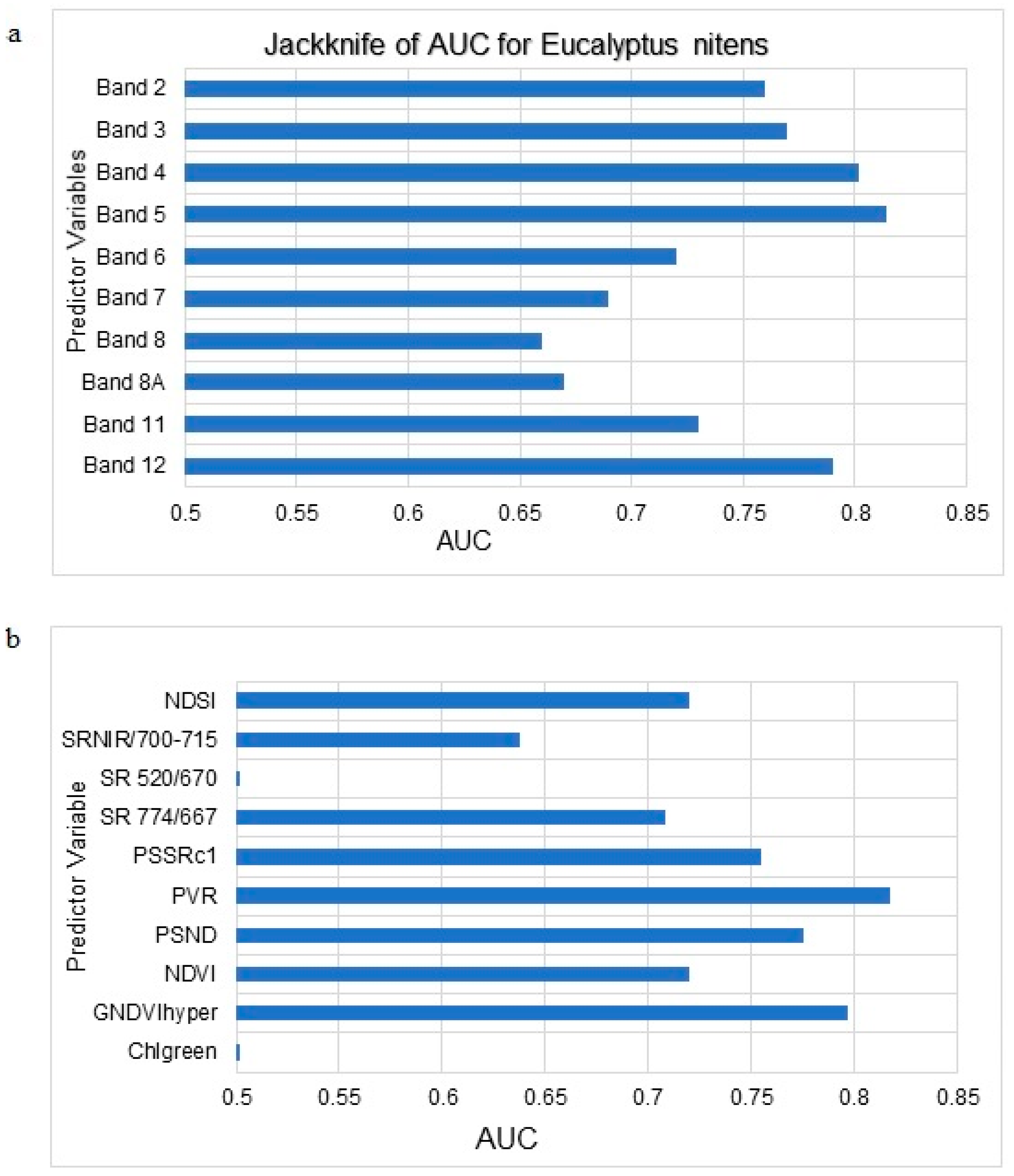
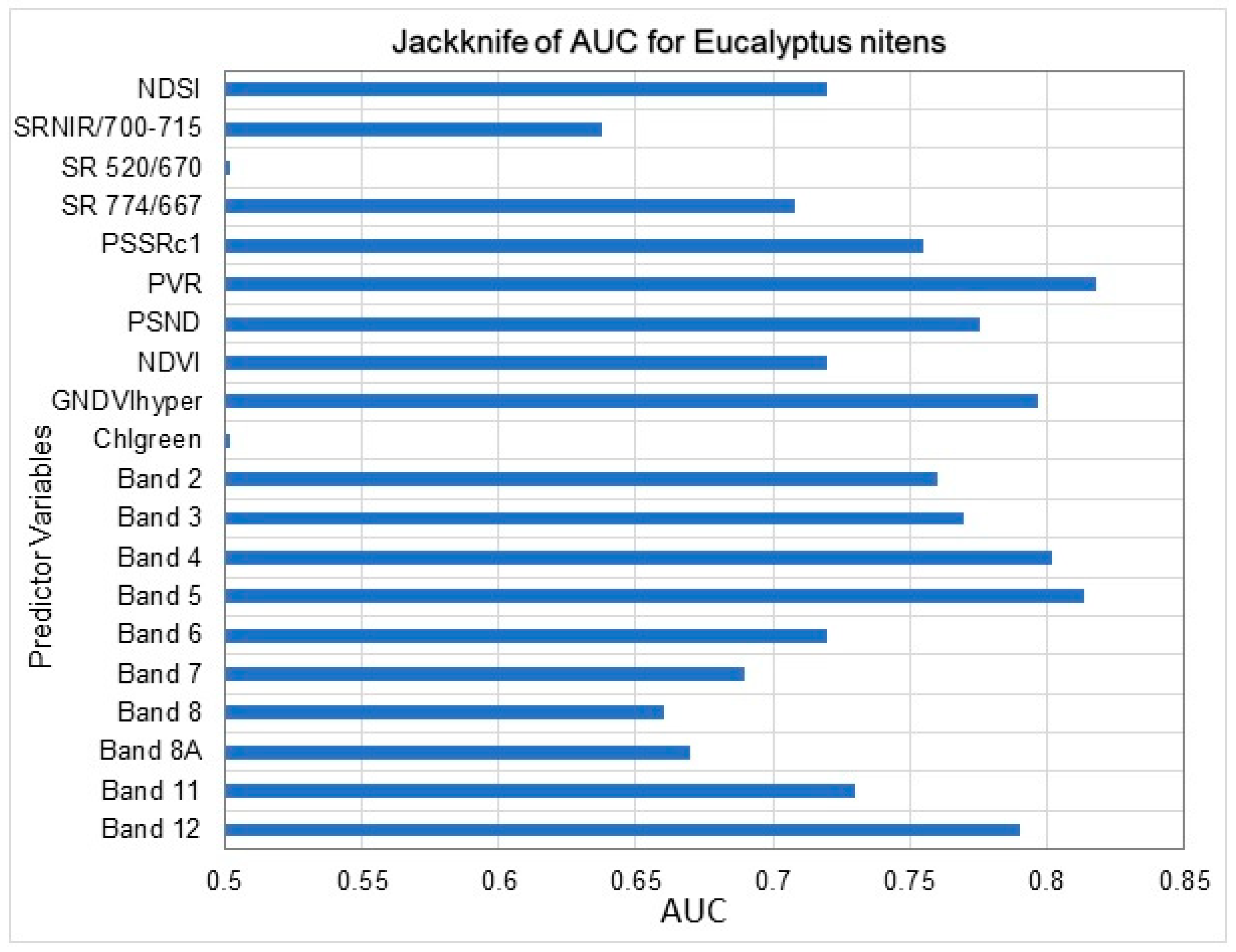
3.1. Maxent Modelling of C. tristis Occurrence

Table 4 shows the results attained after running the three models for determining the probability of the occurrence of the C. tristis. Using spectral bands, an overall accuracy of test data = 0.898 and training data = 0.891 with a TSS value of 0.282 was achieved while vegetation indices produced an overall accuracy of test data = 0.872 and training data = 0.875 with a TSS value of 0.324. When comparing the two models, the overall accuracy decreased by 0.026 test data and 0.04 training data. As a result, Sentinel-2 derived vegetation indices were outperformed by bands in detecting the probability of the occurrence of C. tristis.
The results in Table 4 show that the overall integration of bands and vegetation indices produced higher prediction accuracy in this study. Using the combined data set, the model yielded a high overall accuracy of 0.890 test data and 0.900 training data with a TSS value of 0.344. Bands performed slightly weaker than vegetation indices. Based on the results, the models performed above the random prediction of 0.5 indicating good results.
Respectively in Figure 2, the Maxent model produced a test jack-knife that indicated the relative importance of each variable in the modelling process. In Figure 2a, the most influential bands in the model were Band 5 (Red edge 1), Band 4 (Red), Band 3 (Green), Band 12 (SWIR 3) and Band 2 (Blue) respectively. As illustrated in Figure 2b, PVR, GNDVIhyper, PSND, SR774/667 and NDSI respectively were the most influential variables in the vegetation indices model. Figure 3 is Jack-knife test variable importance graph of combined variables derived in modelling the spatial distribution of the C. tristis.
Band 5 (Red edge 1) contributed significantly to the probability of the occurrence of the C. tristis with a variable importance of 0.814 (Figure 2a). This shows the significance of the vegetation red edge band in discriminating healthy and unhealthy E. nitens trees. Moreover, Band 4 (Red) was the second highest variable with a contribution of 0.802. Band 4 (Red) recorded a decrease in the reflectance indicating the possibility of infested vegetation in the study area. Additionally, Figure 2a illustrates that bands in the VIS had the highest contribution as Band 3 (Green) was the third highest variable with a contribution of 0.793. Moreover, both Bands 11 (SWIR 2) and 12 (SWIR 3) performed well in the modelling of the C. tristis, with Band 12 (SWIR 3) contributing 0.784 as the fourth highest variable. Band 2 (Blue) also yielded a contribution of 0.757 and was the fifth highest variable in the model. In addition, Band 8 (NIR), Band 6 (Red edge 2), Band 7 (Red edge 3) and Band 8A (Narrow NIR) displayed a significant contribution above 0.65 each to the overall model. Sentinel-2 derived bands demonstrated the high potential of predicting the likely spatial distribution of the C. tristis.
As shown in Figure 2b, PVR was the most prominent variable in the model with a contribution of 0.818. The index has the potential to detect any changes in the chlorophyll content and identify weakly active vegetation affected by stress [29]. The results showed that GNDVIhyper was the second highest important variable with a contribution of 0.797. The test jack-knife highlighted that the PSND was the third highest variable that performed well in the model with a contribution of 0.776. Both the NDSI and NDVI performed fairly equally with a contribution of 0.720. The remaining vegetation indices had a contribution above 0.500 in the model. The results obtained using Sentinel-2 derived vegetation indices alone produced slightly lower prediction accuracies when compared to those derived using the spectral bands.
Comparing the results attained in the model 1 and model 2 for each variable, it is evident that contribution accuracies did not significantly increase indicating similar strength in the prediction of the occurrence of C. tristis. Moreover, of all the three models, the results showed that PVR increased its contribution factor to 0.853 while Band 5 (Red edge 1) increased to 0.821 resulting in vegetation indices outperforming the spectral bands. Hence, results showed that vegetation indices (TSS = 0.324) outperformed bands (TSS = 0.282). However, model 3 produced a TSS value of 0.344, which is closer to +1 indicating a higher accuracy. Therefore, the results from model 3 using both bands and vegetation indices established a significant improvement on the overall contribution accuracies integrated into this study. Clearly, the results from the three models that surpassed the random prediction of 0.5 highlighted the great potential of the model to predict the probability of the occurrence of C. tristis. Based on the Jack-knife results obtained from using the bands alone and vegetation indices alone, we ran the final models using the most influential predictor variables and the results for each group are shown in Table 5 below displaying their performance metrics.

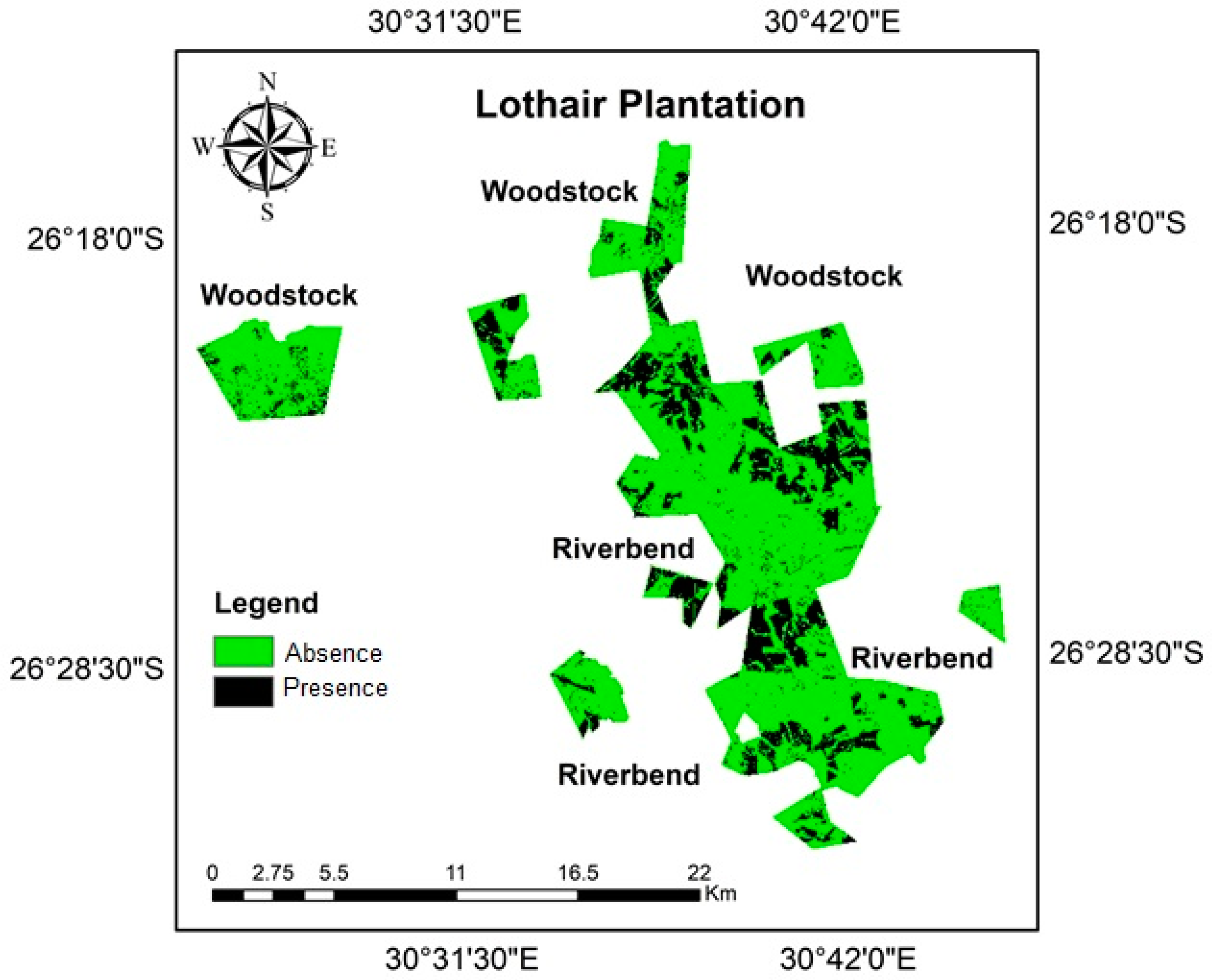
3.2. C. tristis Spatial Distribution

Using the Maxent models, we used both bands and indices to determine the highest probability of C. tristis occurring across the study as illustrated in Figure 4. The highest probability of occurrence is detected in the upper northern parts of the boundary in the Woodstock area descending to the southern areas in the Riverbend area. In the middle of the Riverbend plantation, the highest probability of occurrence is expected, whilst minimum occurrence is anticipated at the lowest parts of the study area. Generally, the presence of the moth is spread across the plantation and observed from the northern parts to southern parts of the study area.

4. Discussion

In this study, using remotely sensed data we modelled the probability of the occurrence of C. tristis on E. nitens through the application of Maxent. Derived Sentinel-2 vegetation indices and bands combined together performed well in modelling the probability the C. tristis occurring. However, when testing both bands and vegetation indices individually, they did not perform as well as the combined variables. The significance of these vegetation indices compared to bands could be explained by their ability to detect the health status of vegetation. C. tristis damages the tree trunk and branches of E. nitens resulting in foliage turning black through chlorosis and then it ultimately dies. As a result, there is a reduction in the absorption rates of the visible light as there are fewer green pigments available, which cause changes in the spectral reflection.
Results obtained in this study regarding the significance of vegetation indices concurs with previous studies of Minařík and Langhammer [54], Metternicht [34] and Hart and Veblen [55]. According to Gitelson and Merzlyak [30], they identified that healthy and unhealthy (stressed) vegetation is mostly observed in the green peak and vegetation red edge region, hence vegetation indices such as PVR and GNDVI yielded an outstanding performance in detecting the probability of C. tristis occurring. In addition, Metternicht [34] highlighted that PVR detects any changes in the reflective properties originating from changes in chlorophyll content and produce low values for photosynthetically weakly active vegetation. Moreover, Gitelson et al. [29] stated that new vegetation indices such as GNDVIhyper have an extensive dynamic range compared to NDVI, hence, they are more sensitive to chlorophyll changes. Therefore, this accounts for the high results yielded by GNDVIhyper in predicting the probability C. tristis occurring in this study. Sanchez-Azofeifa et al. [56] pointed out that SR and NDVI indices are used to estimate the chlorophyll concentration of vegetation as well as observing fundamental variations on leaf age, henceforth, these attributes boosts its performance. Findings from this study showed that SR800/500, SR 774/667 and NDVI performed exceptionally well and can be credited to the above-mentioned. In addition, a combination of two robust bands (NIR and Red) strengthens the probability of modelling and picking up vegetation characteristics that indicate the occurrence of pests. Therefore, different studies have stated that the integration of NIR and band 4 (NDVI) and vegetation indices derived from the red edge bands have enhanced the prediction of pests [19,21,54]. For example, Hart and Veblen [56] illustrated that the vegetation indices were the most important predictors to detect tree mortality caused by spruce beetle (Dendroctonus rufipennis) at grey-stage. Therefore, future studies should seek to improve the detection of C. tristis and its associated impacts on E. nitens trees using powerful vegetation indices.
The results of this study also revealed that the band 5 (Red edge 1) was significant in determining the probability of C. tristis occurring. There is a high correlation between red edge bands and the chlorophyll content of the leaves, so that the spectral signature of E. nitens after chlorosis due to an attack by the C. tristis is easily detected on the red edge spectrum. Several studies that sought to detect and map the spatial distribution of insect pests affecting forest species confirmed that the red edge region played a significant role in predicting of the occurrence of such pests [19,20,57,58]. In support of these results, Oumar and Mutanga [19], Murfitt et al. [59] and Pietrzykowski et al. [15] concluded that red edge bands perform slightly better than other bands in the detection of insect pests in forest damage. For example, Oumar and Mutanga [19] illustrated that the red-edge and NIR bands of WorldView-2 were sensitive to stress-induced changes in leaf chlorophyll content, therefore, improved the potential to detect T. peregrinus infestations. In this regard, the Sentinel-2’s red edge bands demonstrated its great potential in monitoring the probability of C. tristis occurring, using its higher temporal and spatial resolution.
In determining the probability of the occurrence of C. tristis, results of this study further revealed the significant potential of the SWIR region. This region has the ability to map vegetation statues due to its sensitivity to changes in the water content of vegetation [54,55]. Generally, the larva of C. tristis feeds on the cambium, which is responsible for providing layers of phloem and xylem in E. nitens plantations. Therefore, damage to the cambium affects both phloem and xylem which ultimately alters the movement cycle of water from the roots through the trunk to the leaves of E. nitens trees [54]. This results in foliage and canopy water changes. It induces stress which leads to the reduction of the water content present in the main trunk and branches contributing to the change in colour to black. Subsequently, the variations are then detected effectively in the SWIR portion of the electromagnetic spectrum. This then explains the optimal influence of the band 11 (SWIR 2) and band 12 (SWIR 3) in detecting E. nitens compartments that are vulnerable to C. tristis. Similarly to this study, Senf et al. [60] accurately detected the infestations of bark beetle at the red and grey-attack stage using the SWIR bands which distinguished changes in the water content. In a similar study, Ismail et al. [61] indicated that infestation caused by the S. noctilio on pine trees altered the water balance of the tree and bands within the SWIR captured these changes and improved the overall prediction of the pests’ distribution. Furthermore, Hart and Veblen [55] indicated that in the spruce beetle and mountain pine beetle-infested trees, reflection increased in the SWIR and decreased in NIR due to a decrease in the foliar moisture content.
As a species distribution model (SDM), the Maxent model developed a spatial distribution map that shows the probability of the occurrence of C. tristis across the study area. High levels of presence of the moth spread across from the upper (Riverbend plantation) to the lower (Woodstock plantation) portions of the study area while medium presence along the centre of the study area was recorded. The increase in the presence of the moth from the upper portions to the lower portions might be characterized by the absence of natural enemies and hence, could explain the higher level of infestations. The results were similar to Adam et al. [8] which illustrated that in the upper portion of the study area where there was a high presence of the C. tristis compared to the lower portions indicating that C. tristis is rapidly spreading. However, our results may be affected by the trap density and as a result, future studies should look at better sampling strategies. Hence, distribution maps of the C. tristis can help to formulate and improve on-going monitoring and management efforts to reduce the current infestation of E. nitens forests.

5. Conclusions

This study tested the utility of the new generation Sentinel-2 multispectral instrument in detecting and mapping the probability of the occurrence of C. tristis infestations on E. nitens plantations. Based on the findings of this study, we conclude that bands in the VIS, NIR and SWIR are significant in modelling the probability of the occurrence of C. tristis. These three regions measure the spectral reflectance of vegetation that results in determining the amount of healthy and unhealthy vegetation. Additionally, the red edge bands played a crucial role in the probability of occurrence of C. tristis. Consequently, vegetation indices derived from the VIS/NIR have demonstrated their influence in detecting changes in the chlorophyll concentrations and improving the overall modelling concept in this study. Overall, these results underscore the significance of the Sentinel-2 sensor in detecting C. tristis. The results are a platform towards the detection and mapping of the highest probability of occurrence of C. tristis, using different multispectral sensors and their spatial resolution. The utility of remotely sensed data will improve the monitoring and management strategies used in forecasting the prevalence of pests as well as their spread. Moreover, key stakeholders such as forest managers will be in a position to control the damage of pests and devise proactive measures that are seemingly appropriate. This information is critical for preventing extensive damage in the forestry sector.

Author Contributions

In this article, S.T.K., K.Y.P. and R.T.L. were responsible for the conceptualization, methodology and validation of the study. P.M., K.Y.P. and R.T.L. were the supervisors of S.T.K. K.Y.P. and R.T.L. contributed to writing, reviewing and editing the whole paper. In addition, P.M. was responsible for acquiring funding and R.I. was responsible for the data collection that was used in this project. Lastly, S.T.K. obtained the software and carried out the formal analysis of the data as well as writing the original draft preparation.

Funding

This work was supported by The South African Research Chairs Initiative (SARChI)/UKZN/Rural Agronomy, grant number 86893; partially by the National Research Foundation of South Africa (grant number 114898) and “The APC was funded by Supervisors”.

Acknowledgments

We would like to thank Sappi for allowing us access to field data. Above all we would like to thank Dr. Mbulisi Sibanda for his valuable input throughout each stages of the project.

Conflicts of Interest

The authors declare no conflict of interest.

References

  1. Wingfield, M.J.; Roux, J.; Coutinho, T.; Govender, P.; Wingfield, B.D. Plantation disease and pest management in the next century. S. Afr. For. J. 2001, 190, 67–71. [Google Scholar] [CrossRef]
  2. DAFF. A Profile of the South African Forestry Market Value Chain. 2015. Available online: http://www.nda.agric.za/doaDev/sideMenu/Marketing/Annual Publications/Commodity Profiles/field crops/Forestry Market Value Chain Profile 2016.pdf (accessed on 25 June 2017).
  3. DAFF. Forestry Regulation & Oversight. 2017. Available online: https://www.daff.gov.za/daffweb3/Branches/Forestry-Natural-Resources-Management/Forestry-Regulation-Oversight/Facts-and-Figures/plantationsmore (accessed on 12 August 2017).
  4. Albaugh, J.M.; Dye, P.J.; King, J.S. Eucalyptus and water use in South Africa. Int. J. For. Res. 2013, 2013, 852540. [Google Scholar]
  5. Swain, T.-L.; Gardner, R.A.W. A Summary of Current Knowledge of Cold Tolerant Eucalypt Species (CTE’s) Grown in South Africa; University of Natal, Institute for Commercial Forestry Research: Pietermartizburg, South Africa, 2003. [Google Scholar]
  6. Wingfield, M.J.; Slippers, B.; Hurley, B.P.; Coutinho, T.A.; Wingfield, B.D.; Roux, J. Eucalypt pests and diseases: Growing threats to plantation productivity. South. For. J. For. Sci. 2008, 70, 139–144. [Google Scholar] [CrossRef]
  7. Seta. A Profile of the Forestry and Wood Products Sub-Sector. Available online: http://www.fpmseta.org.za/downloads/FPM_sub-sector_forestry_wood_final.pdf (accessed on 12 August 2017).
  8. Adam, E.; Mutanga, O.; Ismail, R. Determining the susceptibility of Eucalyptus nitens forests to Coryphodema tristis (cossid moth) occurrence in Mpumalanga, South Africa. Int. J. Geogr. Inf. Sci. 2013, 27, 1924–1938. [Google Scholar] [CrossRef]
  9. Boreham, G.R. A survey of cossid moth attack in Eucalyptus nitens on the Mpumalanga Highveld of South Africa. S. Afr For. J. 2006, 206, 23–26. [Google Scholar]
  10. Gebeyehu, S.; Hurley, B.P.; Wingfield, M.J. A new lepidopteran insect pest discovered on commercially grown Eucalyptus nitens in South Africa: Research in action. S. Afr. J. Sci. 2005, 101, 26–28. [Google Scholar]
  11. Bouwer, M.C.; Slippers, B.; Degefu, D.; Wingfield, M.J.; Lawson, S.; Rohwer, E.R. Identification of the sex pheromone of the tree infesting Cossid moth Coryphodema tristis (Lepidoptera: Cossidae). PLoS ONE 2015, 10, e0118575. [Google Scholar] [CrossRef]
  12. FAO. Overview of Forest Pests South Africa; FAO: Rome Italy, 2007. [Google Scholar]
  13. Xing, Z.; Zhang, L.; Wu, S.; Yi, H.; Gao, Y.; Lei, Z. Niche comparison among two invasive leafminer species and their parasitoid Opius biroi: Implications for competitive displacement. Sci. Rep. 2017, 7, 4246. [Google Scholar] [CrossRef]
  14. Pause, M.; Schweitzer, C.; Rosenthal, M.; Keuck, V.; Bumberger, J.; Dietrich, P.; Heurich, M.; Jung, A.; Lausch, A. In situ/remote sensing integration to assess forest health—A review. Remote Sens. 2016, 8, 471. [Google Scholar] [CrossRef]
  15. Pietrzykowski, E.; Sims, N.; Stone, C.; Pinkard, L.; Mohammed, C. Predicting Mycosphaerella leaf disease severity in a Eucalyptus globulus plantation using digital multi-spectral imagery. South. Hemisph. For. J. 2007, 69, 175–182. [Google Scholar] [CrossRef]
  16. Germishuizen, I.; Peerbhay, K.; Ismail, R. Modelling the susceptibility of pine stands to bark stripping by Chacma baboons (Papio ursinus) in the Mpumalanga Province of South Africa. Wildl. Res. 2017, 44, 298–308. [Google Scholar] [CrossRef]
  17. Donatelli, M.; Magarey, R.D.; Bregaglio, S.; Willocquet, L.; Whish, J.P.M.; Savary, S. Modelling the impacts of pests and diseases on agricultural systems. Agric. Syst. 2017, 155, 213–224. [Google Scholar] [CrossRef] [PubMed]
  18. Lottering, R.; Mutanga, O. Optimising the spatial resolution of WorldView-2 pan-sharpened imagery for predicting levels of Gonipterus scutellatus defoliation in KwaZulu-Natal, South Africa. ISPRS J. Photogramm. Remote Sens. 2016, 112, 13–22. [Google Scholar] [CrossRef]
  19. Oumar, Z.; Mutanga, O. Using WorldView-2 bands and indices to predict bronze bug (Thaumastocoris peregrinus) damage in plantation forests. Int. J. Remote Sens. 2013, 34, 2236–2249. [Google Scholar] [CrossRef]
  20. Adelabu, S.; Mutanga, O.; Adam, E.; Sebego, R. Spectral discrimination of insect defoliation levels in mopane woodland using hyperspectral data. IEEE J. Sel. Top. Appl. Earth Obs. Remote Sens 2014, 7, 177–186. [Google Scholar] [CrossRef]
  21. Hojas-Gascon, L.; Belward, A.; Eva, H.; Ceccherini, G.; Hagolle, O.; Garcia, J.; Cerutti, P. Potential improvement for forest cover and forest degradation mapping with the forthcoming Sentinel-2 program. Int. Arch. Photogramm. Remote Sens. Spat. Inf. Sci. 2015, 7, W3. [Google Scholar] [CrossRef]
  22. Immitzer, M.; Vuolo, F.; Atzberger, C. First experience with Sentinel-2 data for crop and tree species classifications in central Europe. Remote Sens. 2016, 8, 166. [Google Scholar] [CrossRef]
  23. Ng, W.-T.; Rima, P.; Einzmann, K.; Immitzer, M.; Atzberger, C.; Eckert, S. Assessing the Potential of Sentinel-2 and Pléiades Data for the Detection of Prosopis and Vachellia spp. in Kenya. Remote Sens. 2017, 9, 74. [Google Scholar] [CrossRef]
  24. Gascon, F.; Bouzinac, C.; Thépaut, O.; Jung, M.; Francesconi, B.; Louis, J.; Lonjou, V.; Lafrance, B.; Massera, S.; Gaudel-Vacaresse, A. Copernicus Sentinel-2A calibration and products validation status. Remote Sens. 2017, 9, 584. [Google Scholar] [CrossRef]
  25. Radoux, J.; Chomé, G.; Jacques, D.; Waldner, F.; Bellemans, N.; Matton, N.; Lamarche, C.; D’Andrimont, R.; Defourny, P. Sentinel-2’s Potential for Sub-Pixel Landscape Feature Detection. Remote Sens. 2016, 8, 488. [Google Scholar] [CrossRef]
  26. Blackburn, G.A. Spectral indices for estimating photosynthetic pigment concentrations: A test using senescent tree leaves. Int. J. Remote Sens. 1998, 19, 657–675. [Google Scholar] [CrossRef]
  27. Carter, G.A. Ratios of leaf reflectances in narrow wavebands as indicators of plant stress. Int. J. Remote Sens. 1994, 15, 697–703. [Google Scholar] [CrossRef]
  28. Zarco-Tejada, P.J.; Miller, J.R.; Noland, T.L.; Mohammed, G.H.; Sampson, P.H. Scaling-up and model inversion methods with narrow-band optical indices for chlorophyll content estimation in closed forest canopies with hyperspectral data. IEEE Trans. Geosci. Remote Sens. 2001, 39, 1491–1507. [Google Scholar] [CrossRef]
  29. Gitelson, A.A.; Merzlyak, M.N.; Lichtenthaler, H.K. Detection of Red Edge Position and Chlorophyll Content by Reflectance Measurements Near 700 nm. J. Plant Physiol. 1996, 148, 501–508. [Google Scholar] [CrossRef]
  30. Gitelson, A.A.; Merzlyak, M.N. Remote estimation of chlorophyll content in higher plant leaves. Int. J. Remote Sens. 1997, 18, 2691–2697. [Google Scholar] [CrossRef]
  31. Gitelson, A.A.; Kaufman, Y.J.; Merzlyak, M.N. Use of a green channel in remote sensing of global vegetation from EOS-MODIS. Remote Sens. Environ. 1996, 58, 289–298. [Google Scholar] [CrossRef]
  32. Richardson, A.D.; Duigan, S.P.; Berlyn, G.P. An evaluation of noninvasive methods to estimate foliar chlorophyll content. New Phytol. 2002, 153, 185–194. [Google Scholar] [CrossRef] [Green Version]
  33. Gitelson, A.A.; Keydan, G.P.; Merzlyak, M.N. Three-band model for noninvasive estimation of chlorophyll, carotenoids, and anthocyanin contents in higher plant leaves. Geophys. Res. Lett. 2006, 33, L11402. [Google Scholar] [CrossRef]
  34. Metternicht, G. Vegetation indices derived from high-resolution airborne videography for precision crop management. Int. J. Remote Sens. 2003, 24, 2855–2877. [Google Scholar] [CrossRef]
  35. Phillips, S.J.; Anderson, R.P.; Dudík, M.; Schapire, R.E.; Blair, M.E. Opening the black box: An open-source release of Maxent. Ecography 2017, 40, 887–893. [Google Scholar] [CrossRef]
  36. Ndlovu, P.; Mutanga, O.; Sibanda, M.; Odindi, J.; Rushworth, I. Modelling potential distribution of bramble (rubus cuneifolius) using topographic, bioclimatic and remotely sensed data in the KwaZulu-Natal Drakensberg, South Africa. Appl. Geogr. 2018, 99, 54–62. [Google Scholar] [CrossRef]
  37. Elith, J.; Graham, C.H.; Anderson, R.P.; Dudík, M.; Ferrier, S.; Guisan, A.; Hijmans, R.J.; Huettmann, F.; Leathwick, J.R.; Lehmann, A.; et al. Novel Methods Improve Prediction of Species’ Distributions from Occurrence Data. Ecography 2006, 29, 129–151. [Google Scholar] [CrossRef]
  38. Biber-Freudenberger, L.; Ziemacki, J.; Tonnang, H.E.Z.; Borgemeister, C. Future Risks of Pest Species under Changing Climatic Conditions. PLoS ONE 2016, 11, e0153237. [Google Scholar] [CrossRef] [PubMed]
  39. Matawa, F.; Murwira, A.; Zengeya, F.M.; Atkinson, P.M. Modelling the spatial-temporal distribution of tsetse (Glossina pallidipes) as a function of topography and vegetation greenness in the Zambezi Valley of Zimbabwe. Appl. Geogr. 2016, 76, 198–206. [Google Scholar] [CrossRef]
  40. Yi, Y.; Cheng, X.; Yang, Z.-F.; Zhang, S.-H. Maxent modeling for predicting the potential distribution of endangered medicinal plant (H. riparia Lour) in Yunnan, China. Ecol. Eng. 2016, 92, 260–269. [Google Scholar] [CrossRef]
  41. Shabani, F.; Kumar, L.; Ahmadi, M. A comparison of absolute performance of different correlative and mechanistic species distribution models in an independent area. Ecol. Evol. 2016, 6, 5973–5986. [Google Scholar] [CrossRef] [PubMed] [Green Version]
  42. Phillips, S.J.; Anderson, R.P.; Schapire, R.E. Maximum entropy modeling of species geographic distributions. Ecol. Model. 2006, 190, 231–259. [Google Scholar] [CrossRef]
  43. Efron, B.; Stein, C. The jackknife estimate of variance. Ann. Stat. 1981, 9, 586–596. [Google Scholar] [CrossRef]
  44. Phillips, S.J.; Dudík, M. Modeling of species distributions with Maxent: New extensions and a comprehensive evaluation. Ecography 2008, 31, 161–175. [Google Scholar] [CrossRef]
  45. Hageer, Y.; Esperón-Rodríguez, M.; Baumgartner, J.B.; Beaumont, L.J. Climate, soil or both? Which variables are better predictors of the distributions of Australian shrub species? PeerJ 2017, 5, e3446. [Google Scholar] [CrossRef]
  46. Molloy, S.W.; Davis, R.A.; van Etten, E.J.B. Incorporating field studies into species distribution and climate change modelling: A case study of the koomal Trichosurus vulpecula hypoleucus (Phalangeridae). PLoS ONE 2016, 11, e0154161. [Google Scholar] [CrossRef] [PubMed]
  47. Tabet, S.; Belhemra, M.; Francois, L.; Arar, A. Evaluation by prediction of the natural range shrinkage of Quercus ilex L. in eastern Algeria. İstanbul Üniversitesi Orman Fakültesi Dergisi 2018, 68, 7–15. [Google Scholar] [CrossRef]
  48. Wang, R.; Li, Q.; He, S.; Liu, Y.; Wang, M.; Jiang, G. Modeling and mapping the current and future distribution of Pseudomonas syringae pv. actinidiae under climate change in China. PLoS ONE 2018, 13, e0192153. [Google Scholar] [CrossRef] [PubMed]
  49. Rebelo, H.; Jones, G. Ground validation of presence-only modelling with rare species: A case study on barbastelles Barbastella barbastellus (Chiroptera: Vespertilionidae). J. Appl. Ecol. 2010, 47, 410–420. [Google Scholar] [CrossRef]
  50. Allouche, O.; Tsoar, A.; Kadmon, R. Assessing the accuracy of species distribution models: Prevalence, kappa and the true skill statistic (TSS). J. Appl. Ecol. 2006, 43, 1223–1232. [Google Scholar] [CrossRef]
  51. Liu, C.; White, M.; Newell, G. Selecting thresholds for the prediction of species occurrence with presence-only data. J. Biogeogr. 2013, 40, 778–789. [Google Scholar] [CrossRef]
  52. Berthon, K.; Esperon-Rodriguez, M.; Beaumont, L.J.; Carnegie, A.J.; Leishman, M.R. Assessment and prioritisation of plant species at risk from myrtle rust (Austropuccinia psidii) under current and future climates in Australia. Biol. Conserv. 2018, 218, 154–162. [Google Scholar] [CrossRef]
  53. Elith, J.; Phillips, S.J.; Hastie, T.; Dudík, M.; Chee, Y.E.; Yates, C.J. A statistical explanation of MaxEnt for ecologists. Divers. Distrib. 2011, 17, 43–57. [Google Scholar] [CrossRef]
  54. Minařík, R.; Langhammer, J. Use of a multispectral UAV photogrammetry for detection and tracking of forest disturbance dynamics. Int. Arch. Photogramm. Remote Sens. Spat. Inf. Sci. 2016, XLI-B8, 711–718. [Google Scholar]
  55. Hart, S.J.; Veblen, T.T. Detection of spruce beetle-induced tree mortality using high- and medium-resolution remotely sensed imagery. Remote Sens. Environ. 2015, 168, 134–145. [Google Scholar] [CrossRef] [Green Version]
  56. Sanchez-Azofeifa, A.; Oki, Y.; Wilson Fernandes, G.; Ball, R.A.; Gamon, J. Relationships between endophyte diversity and leaf optical properties. Trees 2012, 26, 291–299. [Google Scholar] [CrossRef]
  57. Matawa, F.; Murwira, K.S.; Shereni, W. Modelling the distribution of suitable Glossina Spp. habitat in the North Western parts of Zimbabwe using remote sensing and climate data. Geoinform. Geostast. Overv. 2013. [Google Scholar] [CrossRef]
  58. Eitel, J.U.H.; Vierling, L.A.; Litvak, M.E.; Long, D.S.; Schulthess, U.; Ager, A.A.; Krofcheck, D.J.; Stoscheck, L. Broadband, red-edge information from satellites improves early stress detection in a New Mexico conifer woodland. Remote Sens. Environ. 2011, 115, 3640–3646. [Google Scholar] [CrossRef]
  59. Murfitt, J.; He, Y.; Yang, J.; Mui, A.; De Mille, K. Ash decline assessment in emerald ash borer infested natural forests using high spatial resolution images. Remote Sens. 2016, 8, 256. [Google Scholar] [CrossRef]
  60. Senf, C.; Seidl, R.; Hostert, P. Remote sensing of forest insect disturbances: Current state and future directions. Int. J. Appl. Earth Obs. Geoinf. 2017, 60, 49–60. [Google Scholar] [CrossRef]
  61. Ismail, R.; Mutanga, O.; Bob, U. Forest health and vitality: The detection and monitoring of Pinus patula trees infected by Sirex noctilio using digital ultispectral imagery (DMSI). South. Hemisph. For. J. 2007, 69, 39. [Google Scholar] [CrossRef]
Figure 1. (a) Map of South Africa showing the Mpumalanga Province, (b) the location of the study area within the Mpumalanga Province (c,d) show healthy and infested Eucalyptus nitens and (e) shows the sampled compartments over the Sentinel-2 image with a false-colour composite of R-NIR-B (B4, B8 & B2).
Remotesensing 11 00278 g001
Figure 2. Jack-knife test variable importance graph of (a) bands and (b) vegetation indices derived in modelling the spatial distribution of C. tristis.
Remotesensing 11 00278 g002
Figure 3. Jack-knife test variable importance graph of combined variables derived in modelling the spatial distribution of the C. tristis.
Remotesensing 11 00278 g003
Figure 4. Map of C. tristis occurrence predicted with Maxent models using bands and vegetation indices as predictors.
Remotesensing 11 00278 g004
Table 1. Sentinel-2 bands used in this study.
Spatial Resolution (m) Sentinel-2 BandsWavelength (nm) Bandwidth (nm)
Band 2—Blue496.698
10Band 3—Green560.045
Band 4—Red 664.538
Band 8—NIR835.1145
Band 5—Vegetation Red Edge 703.919
Band 6—Vegetation Red Edge
Band 7—Vegetation Red Edge
Band 8a—Narrow NIR
740.2
782.5
864.8
18
28
33
20Band 11—SWIR (2)1613.7143
Band 12—SWIR (3)2202.4242
Table 2. Sentinel 2 vegetation indices tested in this study.
Vegetation Indices AbbreviationEquationIndex EquationReference
Simple Ratio 800/500 Pigment specific simple ratio C1PSSRc1 NIR Blue B 8 B 2 [26]
Simple Ratio 520/670SR520/670 Blue Red B 2 B 4 [27]
Simple Ratio 774/677SR774/677 Vegetation   Red   Edge Red B 7 B 4 [28]
Simple Ratio NIR/700–715SRNir/700–715 Water   vapour   Vegetation   Red   edge B 9 B 5 [29]
Normalized Difference Vegetation IndexNDVI NIR Red NIR + Red B 8 B 4 B 8 + B 4 [30]
Normalized Difference 780/550 Green NDVI hyperGNDVIhyper Vegetation   Red   edge Green Vegetation   Red   edge + Green B 7 B 3 B 7 + B 3 [31]
Normalized Difference Salinity IndexNDSI SWIR 2 SWIR 3 SWIR 2 + SWIR 3 B 11 B 12 B 11 + B 12 [32]
Normalized Difference 800/470 Pigment specific normalized difference C2PSNDc2 NIR Blue NIR + Blue B 8 B 2 B 8 + B 2 [26]
Chlorophyll GreenChlgreen { Vegetation   Red   edge Green } 1 { B 7 B 3 } 1 [33]
Normalized Difference 550/650 Photosynthetic vigour ratioPVR Green Red Green + Red B 3 B 4 B 3 + B 4 [34]
Table 3. Bands and indices from Sentinel-2A MSI data used as independent variables for predicting the probability of occurrence of the C. tristis with Maxent models.
Model
Scenarios
Sentinel-2A Bands and Indices List of Variables Used
1Spectral bandsBand 2, Band 3, Band 4, Band 5, Band 6, Band 7, Band 8, Band 8A, Band 11 and Band 12
2Vegetation indices PSSRc1, SR520/670, SR774/677, SRNir/700-715, NDVI, GNDVIhyper, NDSI, PSNDc2, Chlgreen and PVR
3Combined variablesBands and vegetation indices
4The most influential bands Band 5, Band 4, Band 3, Band 12, Band 2, PVR, GNDVIhyper, PSND, SR774/667 and NDSI
Table 4. Evaluation results for all Maxent models used for predicting the probability of the occurrence of C. tristis.
Predictor VariablesModel Accuracy
AUCTSS
Training Testing
Bands 0.8910.8980.282
Vegetation indices 0.8750.8720.324
Combined variables 0.9000.8900.344
Table 5. Evaluation results for all influential predictor variables used for predicting the probability of occurrence of the C. tristis.
Predictor VariablesModel Accuracy
AUCTSS
Training Testing
Bands 0.8580.8490.482
Vegetation indices 0.8680.8670.564
Combined variables 0.8690.8720.581

