Article

Validating a Landsat Time-Series of Fractional Component Cover Across Western U.S. Rangelands

1
AFDS, Contractor to the U.S. Geological Survey (USGS) Earth Resources Observation and Science Center, Sioux Falls, SD 57198, USA
2
U.S. Geological Survey (USGS) Earth Resources Observation and Science Center, Sioux Falls, SD 57198, USA
3
KBRwyle, Contractor to the U.S. Geological Survey (USGS) Earth Resources Observation and Science Center, Sioux Falls, SD 57198, USA
*
Author to whom correspondence should be addressed.
Remote Sens. 2019, 11(24), 3009; https://doi.org/10.3390/rs11243009
Submission received: 14 November 2019 / Revised: 10 December 2019 / Accepted: 12 December 2019 / Published: 13 December 2019

Abstract

:
Western U.S. rangelands have been quantified as six fractional cover (0%–100%) components over the Landsat archive (1985–2018) at a 30 m resolution, termed the “Back-in-Time” (BIT) dataset. Robust validation through space and time is needed to quantify product accuracy. Here, we used field data collected concurrently with high-resolution satellite (HRS) images over multiple locations (n = 42) and years. Field observations were used to train regression tree models, predicting the component cover across each HRS image. Our objectives were to evaluate the spatial and temporal relationships between HRS and BIT component cover and compare spatio-temporal climate responses. First, for each HRS site-year (n = 77) we averaged both the HRS and BIT predictions within each site separately and regressed the averages to quantify the temporal accuracy. Next, we regressed individual pixel values of corresponding HRS and BIT predictions to quantify the spatio-temporal accuracy. Results showed strong temporal correlations with an average R2 of 0.63 and Root Mean Square Error (RMSE) of 5.47% as well as strong spatio-temporal correlations with an average R2 of 0.52 and RMSE of 7.89% across components. Our approach increased the validation sample size relative to direct comparison of field observations. Validation results showed robust spatio-temporal relationships between HRS and BIT data, providing increased user confidence in the data.

1. Introduction

Rangelands of the Western U.S. have recently been quantified as a series of fractional cover components [1,2]. The products were developed using extensive field observations to model fractional cover on high-resolution satellite (HRS) image (with a 2 m resolution) footprints. HRS predictions of component cover were downscaled to serve as training for regional-scale predictions using Landsat imagery. These regional maps have recently been completed for most rangelands in Western U.S., representing a nominal date of 2015.
Static maps of fractional vegetation cover are useful for a variety of applications however, they cannot provide information on the temporal trends in rangeland condition or the nature of the change processes [3,4,5]. We developed a method to produce fractional vegetation maps, similar to the nominal 2015 product, over the Landsat 5–8 archive (1985–2018) across large spatial extents [4,5]. This “Back-In-Time” (BIT) product suite consists of annual fractional cover (0%–100%) maps of shrub, sagebrush (Artemisia spp.), herbaceous, annual herbaceous, litter, and bare ground cover. These products were found to have robust responses to climate drivers (precipitation and temperature) and disturbance in the Northern Great Basin [4,5]. While most change in fractional component cover was small (<10% cover change over the study period), a large majority of pixels indicated at least some change [5]. The BIT suite was designed to capture spatially discrete abrupt change and pervasive gradual change [5] that is often ignored by the remote sensing community [6].
Validation of any remotely sensed mapping application is critical to increasing user confidence in products, foster usage in management decisions, and determine the more robust estimate in cases of competing datasets [7,8]. However, validation is often challenging [3,6,9,10,11], especially with time-series maps [12]. Validation is often somewhat subjective, relying on manual image interpretation on reference blocks [13], Google Earth time-series imagery [14,15], or case studies. Most validation methods are designed for thematic classes (e.g., [10,15]) that typically employ confusion matrices to understand accuracies [14]. An introduction of more mapping classes often results in weaker validation results [15]. By extension, validation of fractional component time-series pose the most difficult scenario, particularly in areas of subtle change. This is especially true in dryland ecosystems with frequently sparse vegetation canopies that increase the influence of soils and senesced vegetation and where only a scarce ground-based data network exists [16]. Major challenges to time-series validation include (1) validation datasets that are not directly comparable to the remotely sensed data, (2) sample size, spatial extent, or temporal extent of validation datasets, which are limited, (3) validation datasets that are not independent, and (4) appropriate data do not exist as field sampling is highly resource intensive [17,18]. Ideally, validation datasets should be one step closer to the ground truth (e.g., HRS imagery) than evaluated broad-scale products [3,19].
We previously validated the BIT suite using a variety of methods. First, both Shi et al. and Rigge et al. identified pseudo-invariant pixels where no cover change should occur due to high amounts of bare ground cover [4,5]. These sites typically occurred in talus slopes, lava flows, or rock faces. Both observed bare ground cover of ~100% and no significant trends in these pseudo-invariant sites. Second, Shi et al. found that BIT products responded as expected to fire, with increasing component cover change detected in more severe monitoring trends in ‘burn severity’ burns [4]. Individual components responded as expected to fire; i.e., increased bare ground and litter cover and decreased shrub cover. Third, Rigge et al. compared Assessment, Inventory, and Monitoring (AIM) plots collected by the Bureau of Land Management (BLM) in 2011, 2013, 2014, and 2015 to the corresponding BIT pixels [5]. This work yielded weak-moderate relationships, with an average coefficient of determination (R2) of 0.24 across components.
The most robust validation conducted to date occurred in southwest Wyoming at two long-term monitoring sites [20]. At these sites, fractional component cover was observed in the field at 126 plots for 10 years during the period of 2006–2018. Field observations and BIT data responded similarly to interannual variation in precipitation, and the field and BIT data had robust temporal and spatio-temporal correlations, with an average R2 of 0.46 across components [20].
Here, we leverage field data observed concurrently with HRS imagery over multiple years and locations in Western U.S. to dramatically expand the spatial extent and sample size of validation analysis relative to a direct comparison to field observations and to previous work. We compare HRS and BIT data in the corresponding space and time. Our objectives were to evaluate the temporal and spatio-temporal relationships between HRS and BIT data, and to compare their response to spatio-temporal variation in climate. We hypothesize that strong temporal and spatio-temporal relationships will exist between HRS and BIT data and that they will exhibit similar climate response.

2. Materials and Methods

2.1. Method Overview

We evaluated a total of 42 HRS sites across the Western U.S. with 32 sites in Wyoming, and 5 sites each in Nevada and Montana. HRS sites span a broad range of vegetation, biophysical, climatic, and disturbance regimes (Figure 1). Our HRS sites were strategically located to collectively capture the range of biophysical conditions within a region [2]. A total of 5 U.S. Environmental Protection Agency (EPA) Level III ecoregions were included in the study area: the Central Basin and Range, Northern Basin and Range, Northwestern Great Plains, Southern Rockies, and Wyoming Basin. Water year (defined as 1 October to 30 September of the following year) precipitation totals at HRS sites in measured years ranged from 149 to 681 mm, water year maximum temperature averages ranged from 9.6 to 17.3 °C, and water year minimum temperature averages ranged from −6.5 to 2.2 °C.
Field data were used to train 2 m predictions of fractional component cover at each HRS site and year. The 2-m predictions were degraded to 30 m, and some were used to train regional Landsat-scale, 30 m, “base” maps of fractional component cover representing circa 2016 conditions. A Landsat-imagery time-series spanning 1985–2018, excluding 2012, was analyzed for change through time. Pixels and times identified as changed from the base were trained using the base fractional component cover from the pixels identified as unchanged. Changed pixels were labeled with the updated predictions, while the base was maintained in the unchanged pixels. The resulting BIT suite includes the fractional cover of the 6 components described above for 1985–2018. We compared the two datasets, HRS and BIT, in space and time.

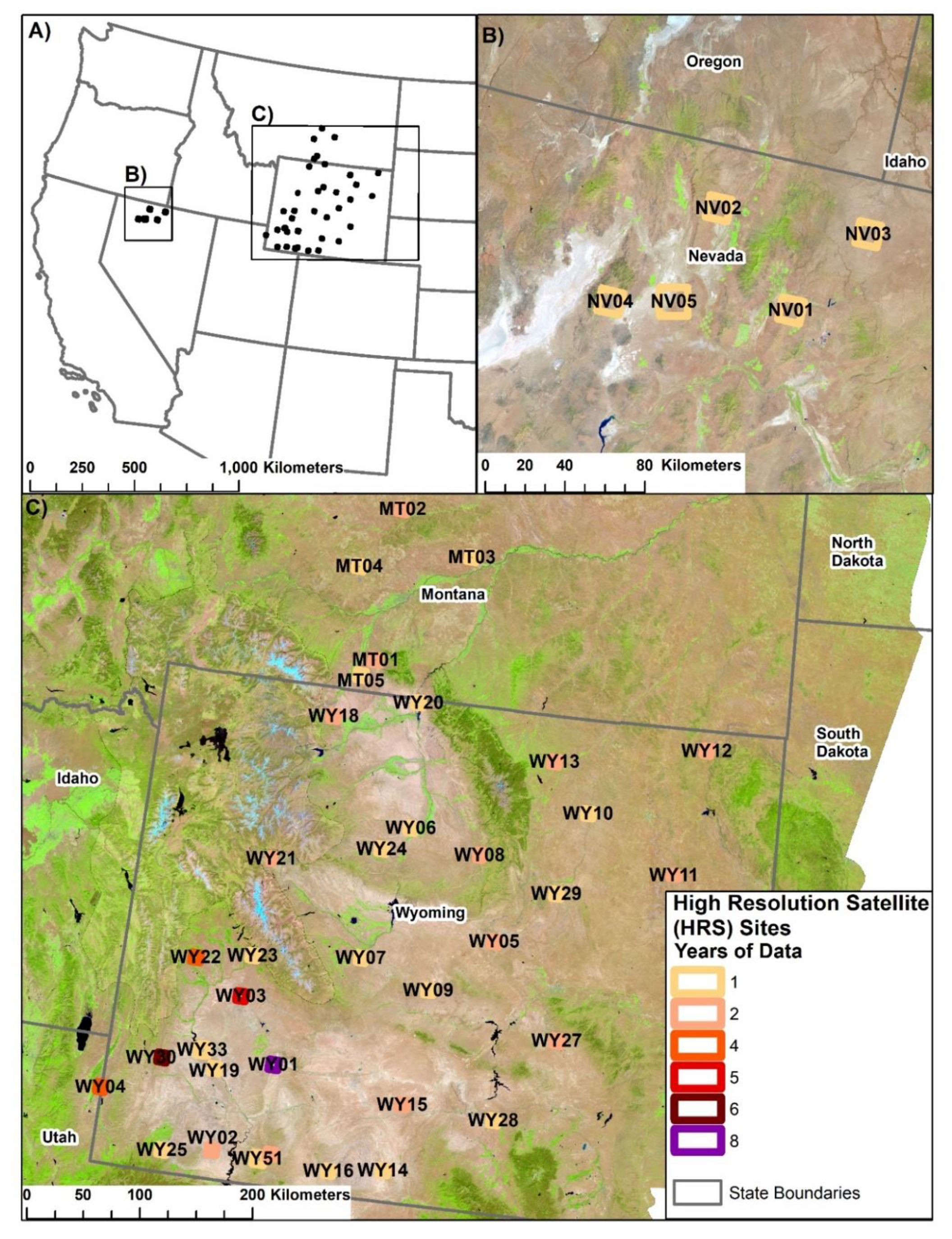
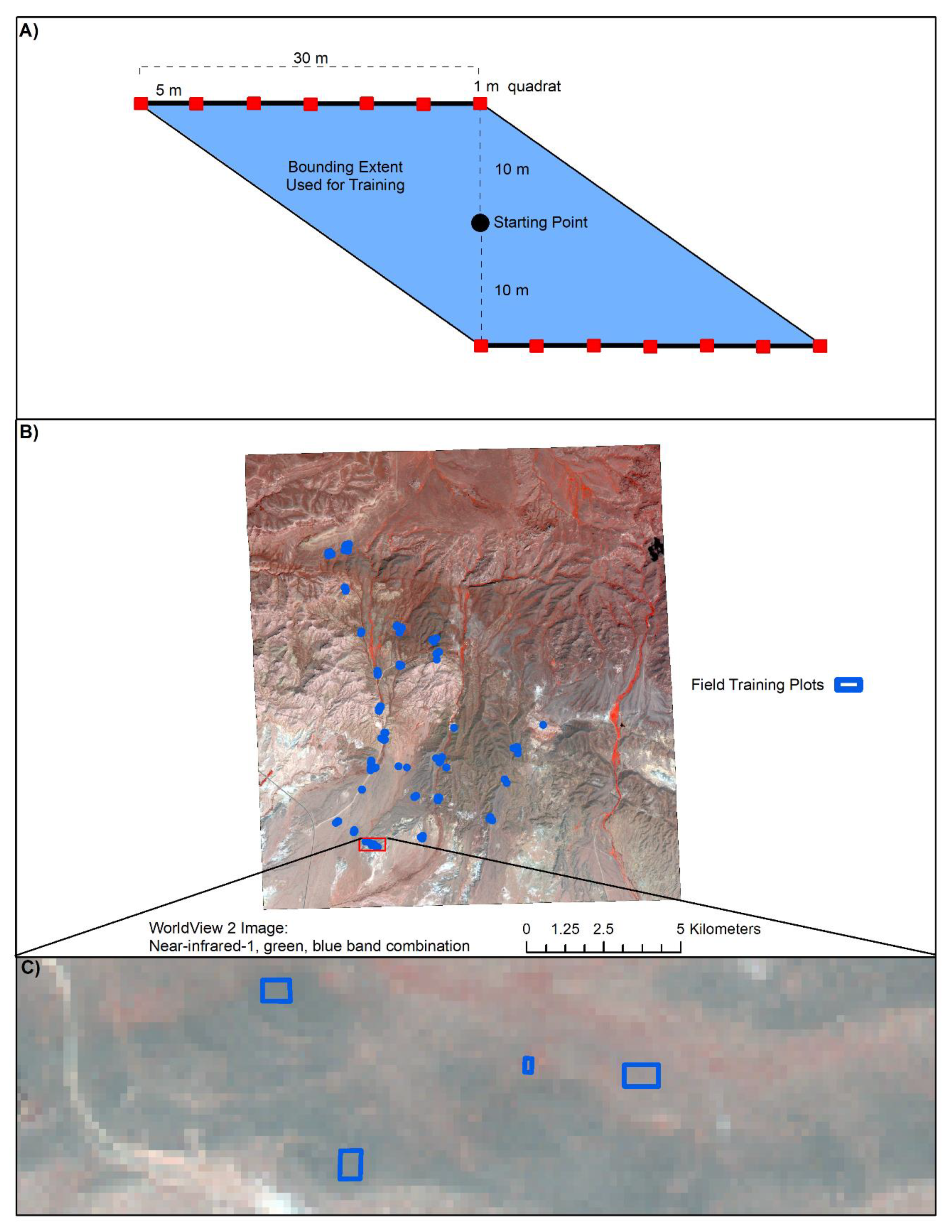
2.2. Field Observations

Field data were collected at HRS sites for each evaluated year (Table 1). We recorded an ocular estimate of each targeted component cover from an overhead perspective and noted the dominant species within each plot. The fractional cover of shrub, sagebrush (Artemisia spp.), herbaceous, annual herbaceous, litter, and bare ground was measured. The sum of the primary components (shrub, herbaceous, litter, and bare ground) equaled 100% in all plots. Data collection occurred within the growing season of May–September and at HRS sites with multiple years we conducted repeat measurement(s) on approximately the same date(s). We used two plot designs over the study period [1,2]. Field data from all sites in 2006–2014, site WY01 in 2015–2017, and WY03 in 2015 were collected at predetermined monitored locations. Plots were selected based on segmentation of HRS imagery to represent the variability of the entire site [21,22]. Segmentation was used to classify each HRS image separately as 30 unsupervised clusters to identify spectrally similar polygon patches for ground sampling [22]. Plots were measured using two 30-m plot transects that each contained seven 1-m2 quadrats spaced every 5 m, for 14 quadrats in total for the plot (Figure 2). At each plot, the observations were averaged across all 14 quadrats. The polygon bounding the transects was converted to raster format with 2-m resolution (Figure 2A). Each 2-m pixel within the polygon was assigned the average value for each component. These rasterized data served as training for HRS predictions. At each HRS site, a total of ~60 plots were measured.
In 2015, plots were selected ad hoc by field crews to represent the range of vegetation, topography, disturbance, and soil color within each HRS site (Figure 2B). The 2015 data in WY01 and WY03 were collected using the previously described method. Field plots at all other sites in 2015 were drawn in the field on a tablet displaying high-resolution imagery to identify patches of ground cover. We again measured the cover of shrub, sagebrush, herbaceous, annual herbaceous, litter, and bare ground cover from an overhead perspective, using ocular estimation. Plots were at minimum 4-m2 in size, and averaged 32-m2, with an average of ~70 plots collected per HRS site (Figure 2C). At each site, we rasterized the plot data to a 2-m resolution to serve as training for HRS predictions.

2.3. HRS Prediction

HRS sites were typically ~8 km by 8 km in size but varied based on the imagery source. All sites had at least one high-resolution image, and some had up to eight. In sites with repeat imagery, we used only the intersecting area among all images, resulting in discrepancies from the typical 8 by 8 km size. We used four sources of high-resolution satellite imagery: QuickBird, RapidEye, Pleiades, and WorldView 2/3 (Table 1 and Table 2). HRS imagery was obtained in several spatial resolutions (Table 2), but all were resampled to 2-m resolution using the nearest neighbor approach. Imagery was ordered for a date corresponding with field data collection, mostly in June and July (Table 1). Satellite scheduling conflicts sometimes resulted in imagery acquisition later than our desired window. HRS images were orthorectified using ERDAS functionality and topographically checked and if needed registered using National Agriculture Imagery (NAIP) orthoimagery.
Rasterized field data were used to train Cubist Regression Tree (RT) [23] algorithms to predict the cover of nine components on HRS images at 2-m resolution [1,2]. Our default settings in Cubist develop models based on a committee of 10 members, with a maximum of 500 rules and 10% extrapolation of the training data’s range of values. For each HRS imagery source, we used all available bands as the independent variable in the Cubist models. Classification of field observations at a 2 m resolution was robust, with cross-validation values typically > R2 = 0.80, often > R2 = 0.90 for bare ground. Next, we identified and excluded non-rangeland areas from HRS predictions including urban areas, agriculture, water, and forest. Cloud, cloud shadows, and snow cover present on HRS imagery were also identified and excluded. All 2-m predictions were resampled to 30-m using cubic convolution, giving the mean value for each 30-m pixel, ignoring excluded non-rangeland areas. While scaling up field observations to a 30-m resolution can introduce noise [24], misregistration of HRS imagery is also a potential problem [8,17], which is partly remedied by upscaling. Our approach has been well vetted [1,2], and dramatically increases the statistical power of validation analyses. In this analysis, we only include the components of shrub, sagebrush, herbaceous, litter, and bare ground, as these components were universally predicted at all HRS sites.

2.4. Base Map

Upscaled HRS predictions were used to train regional Cubist RT models predicting fractional component cover. Independent variables in these models included three seasons of Landsat imagery, representing pre-peak greenness, peak-greenness, and leaf-off phenological stages. We also included topographical variables: Slope, aspect, position index, and several spectral indices (normalized difference built-up index (NDBI, Equation (1)), soil-adjusted vegetation index (SAVI, Equation (2)), and normalized difference water index (NDWI, Equation (3)) developed from each seasonal image. The position index represents the hydrological position of the pixel within the local landscape, with low values for pixels primarily receiving an inflow of surface runoff and high values for pixels primarily with outflow.
NDBI = Shortwave   infrared Near   infrared Shortwave   infrared + Near   infrared
SAVI = Near   infrared Red Near   infrared + Red + 1.5 × ( 1.5 )
NDWI = Near   infrared Shortwave   infrared Near   infrared + Shortwave   infrared
Similar to the high-resolution scale, we identified non-rangeland areas on the Landsat imagery, and excluded them for our predictions. Regional predictions were validated using both independent and cross-validation methods and mosaicked across the Western U.S. [1,2] to produce the “base” map for each component. The HRS sites analyzed in the current manuscript are located in the Wyoming, Black Hills, and Montana regions that were mapped in 2015, and the Northern Great Basin region that was mapped in 2014. Only HRS predictions from these years were included as training in regional base predictions. HRS sites mapped only in 2014 or 2015 constituted most of the training data for base maps and are not included in our validation analysis.

2.5. BIT Predictions

We used BIT fractional component data developed from a Landsat imagery time-series produced using an improved method of Shi et al. and Rigge et al. [4,5]. Briefly, BIT data were developed by obtaining a summer and fall image from each year in the Landsat 5–8 archive (1985–2018). The year 2012 was excluded due to the lack of quality Landsat data, with only Scan Line Corrector (SLC) off data from Landsat 7 available. Next, we used a change vector and change fraction approach [5] to identify spectral change between each summer image with the base year (2014/2015) summer image and between each fall image with the base year fall image. Only change identified in both seasons was maintained. We randomly selected 120,000 points within the non-changed areas identified in each year to serve as training for predicting the fractional component cover in changed areas. We pooled training data in non-changed areas across all years in the time-series and used a series of procedures to remove the most spatially and temporally common values. Doing so resulted in improved predictions by expanding the histograms of the training data and independent variables. The pooled training data were used to develop a spatio-temporal Cubist RT model for each component. Independent variables in each model included the summer and fall Landsat imagery, and the same suite of topographic variables and spectral indices used in base mapping. RT models were developed spatio-temporally but were separately applied to single years of imagery. Fractional component outputs of the RT models were maintained in the area detected as changed in each respective year while the base map was maintained in the unchanged area. We used a series of post-processing models to ensure accurate post-burn trajectories, eliminate noise and illogical change in the predictions, and to remove pixels that were inundated by water at any point in the time-series. All BIT processing occurred on individual Landsat path-rows, which were subsequently mosaicked to a regional level. The final BIT product suite consists of annual maps of shrub, sagebrush, herbaceous, annual herbaceous, litter, and bare ground from 1985–2018, mosaicked to a regional level.

2.6. Data Analysis

Though we geometrically corrected each image, spatial registration of HRS data may vary among years, and when compared to BIT data. To account for this potential variation, the HRS and BIT datasets were compared temporally and spatio-temporally. The temporal analysis removed essentially all impacts of spatial mis-registration by analyzing means across large HRS sites. While the spatio-temporal analysis could be impacted by registration issues, it is made more robust through a direct comparison of a very large number of individual HRS and BIT pixel values. Moreover, the spatio-temporal analysis is not subject to the inflation of regression statistics that can occur when regressing means against means in the temporal analysis. HRS predictions have high, but not perfect accuracy, but still provide an invaluable validation reference [3].
First, for each HRS site-year (n = 77) we averaged both the HRS and BIT prediction based on a sample of 10,000 random points within each site. We excluded areas identified as non-rangeland in either the HRS or BIT dataset and areas identified as cloud/cloud shadow/snow in the HRS dataset. We then plotted the site average HRS and BIT component covers against each other to quantify temporal accuracy. Regression (n = 77) statistics of R2, root-mean square error (RMSE), and p-value were calculated for each component. Some (n = 17) HRS site-years were used to train the base map, which itself is a major input to the BIT process. To test for the influence of potential circularity, we also plotted regression statistics for 2015 used to train base predictions separately from all other data (Table 3).
Next for the spatio-temporal analysis, we plotted individual pixel values of corresponding HRS and BIT predictions against each other, aggregated across space and time at 770,000 points. Data from all HRS sites and years were included. Again, we calculated regression statistics: R2, root-mean square error (RMSE) given in units of percent cover, and p-value were calculated for each component. Finally, we compared the spatio-temporal response of both datasets to Daymet climate variables [25] resampled to 30 m. We evaluated four climate variables: Water year total precipitation (WYPRCP), water year mean maximum temperature (WYTMAX), water year mean minimum temperature (WYTMIN), and growing season (April–September) total precipitation (GSPRCP). Temporal analysis was performed using Microsoft Excel and spatio-temporal analyses in R.

3. Results

3.1. Temporal Correlations

Temporal correlations between HRS and BIT were all robust and significant (p < 0.05), with BIT data accurately representing temporal variation in ground cover as observed by HRS imagery (Figure 3). Bare ground was the top performer (R2 = 0.82, RMSE = 6.78%), while shrub (R2 = 0.63, RMSE = 4.20%) and herbaceous (R2 = 0.74, RMSE = 6.71%) were also strongly related. Across components, the mean temporal correlation was a R2 of 0.63 and RMSE of 5.47%. A total of 17 site-years of HRS data from 2015 in the Wyoming and Montana sites (Figure 1B) was used as training for the base mapping, which in turn was used to train the BIT predictions. Temporal correlations including data from only 2015 sites were somewhat stronger than for data pooled from all other years (Table 3), though all correlations were significant in both pools of data.

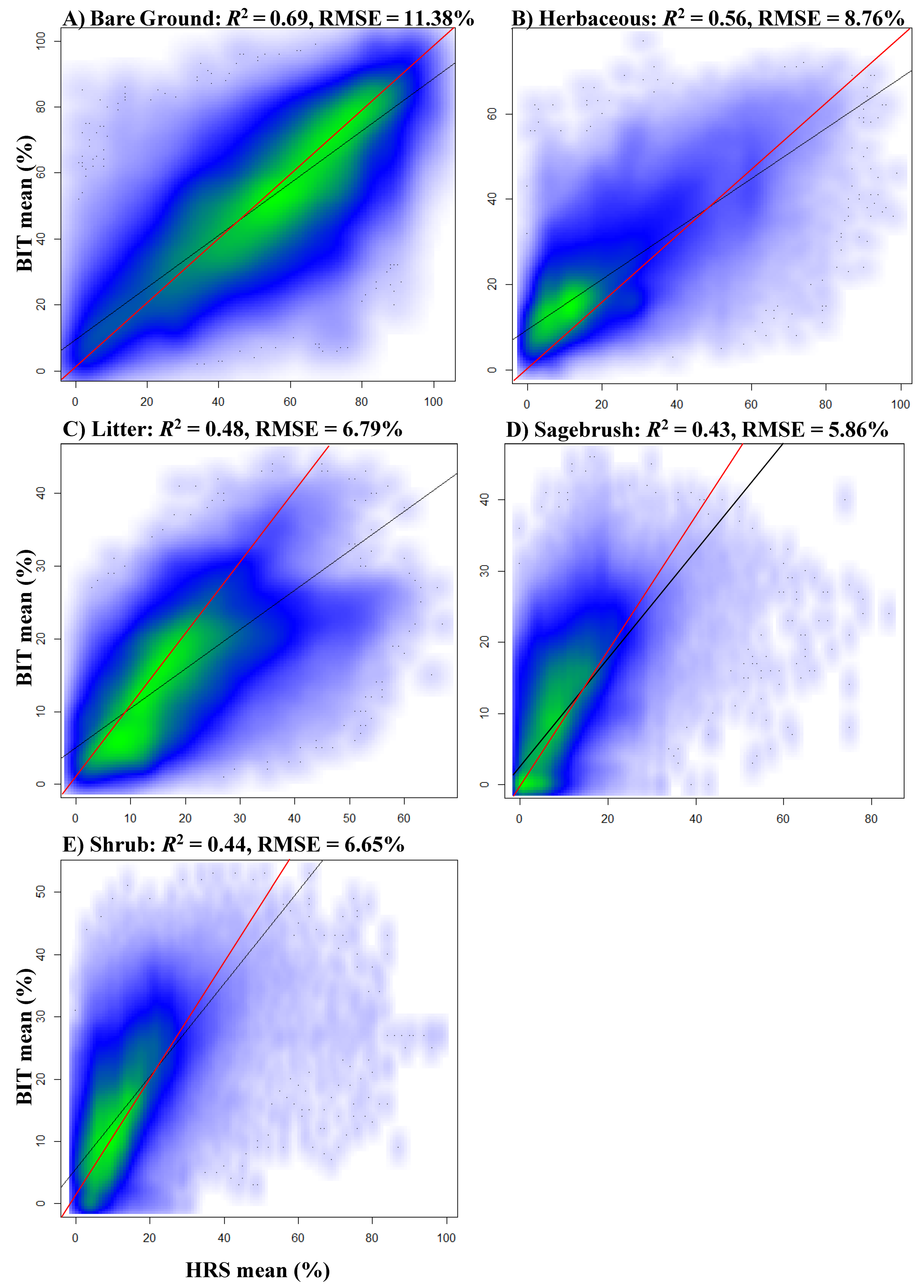
3.2. Spatio-Temporal Correlations

To be of value to users, BIT data must be accurate in both the spatial and temporal dimensions. We found strong spatio-temporal correlations between HRS and BIT data (Figure 4). Across components, the average R2 and RMSE was 0.52% and 7.89%, respectively, and all relationships were significant (p < 0.05). As with the temporal correlations, bare ground was the best performer (R2 = 0.69, RMSE = 11.38%). Bias did exist in the spatio-temporal relationships, where BIT components tended to over-predict the low end of each component range and under-predict the high-end relative to HRS data (see 1:1 line relative to line-of-best fit in Figure 4).

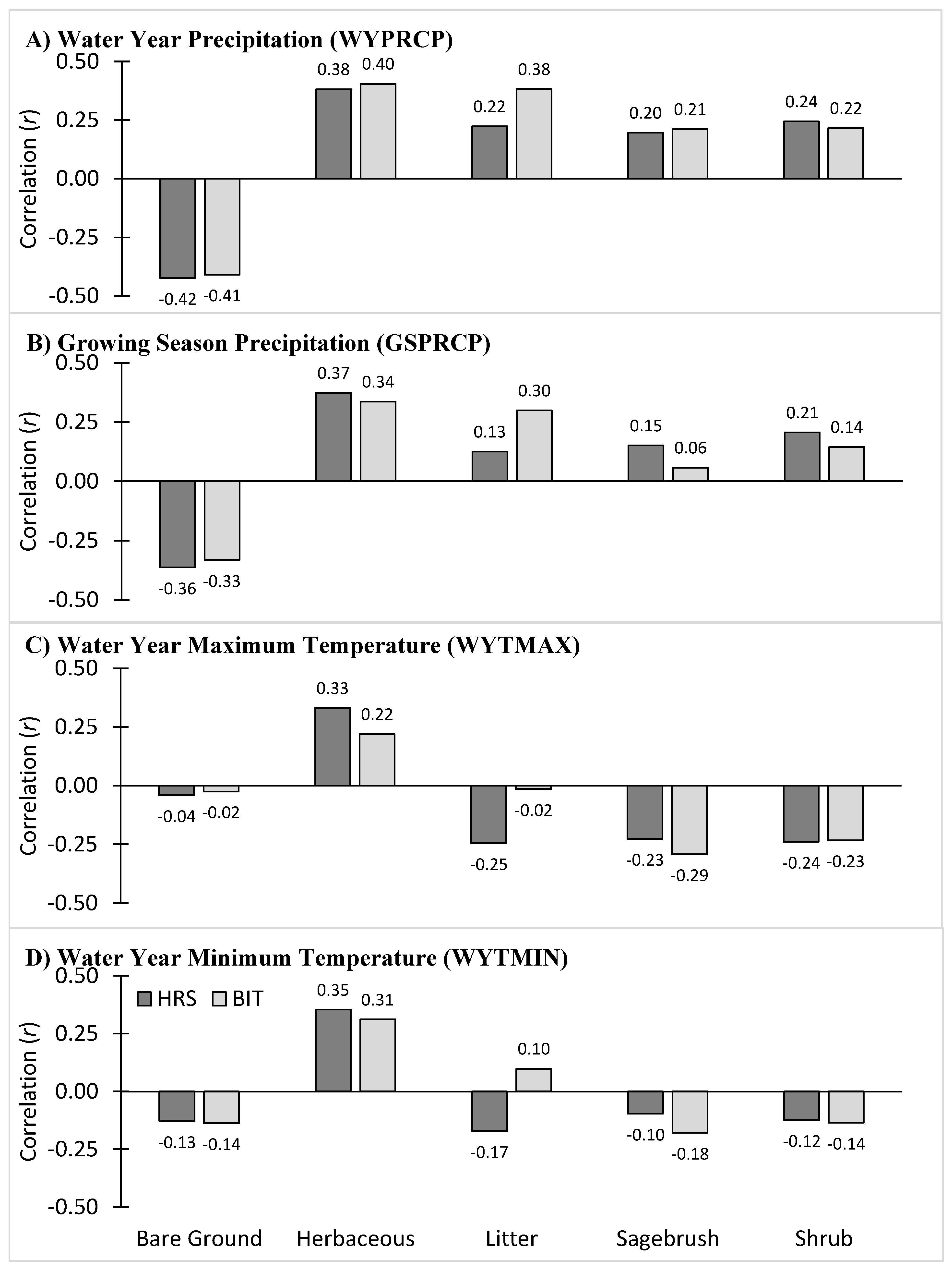
3.3. Climate Relationships

Climate relationships were similar between the HRS and BIT data and the direction of relationships was as expected (Figure 5). Bare ground was negatively related to WYPRCP in both the HRS data (r = −0.42) and BIT data (r = −0.41) (Figure 5A). The HRS data tended to have slightly higher overall mean absolute relationship with climate (r = 0.23) than BIT data (r = 0.22), but in comparison to WYPRCP alone, BIT data had stronger relationships (r = 0.32) than HRS data (r = 0.29). Litter withstanding, the directions of climate relationships in all components followed expectations in both datasets. While some climate relationships were quite weak (e.g., bare ground with WYTMAX), all were significant (p < 0.05) because of the large sample size.

4. Discussion

The temporal relationships between HRS and BIT data were strong across a broad range of vegetation types, disturbance histories, and management practices in the study area. The strength of the correlations, combined with low RMSE values, indicate that the BIT process accurately captured the vegetation characteristics of a site as both a snapshot in time and with regard to its temporal dynamics. However, some HRS site-years occurred as outliers in the correlations. These can be explained in large part by the less-than-ideal dates of high-resolution imagery acquisition. For example, the image for site WY28 in 2007 was acquired on 10 October (Table 1), far past the period of peak greenness targeted. This date of acquisition likely resulted in a low mean predicted herbaceous cover in the HRS data (6.02%) compared to the BIT data (16.98%). The BIT mean component cover values were likely closer to the true value than the HRS data in this case.
Bare ground was the overall top performer in both the temporal (Figure 3) and spatio-temporal (Figure 4) correlations, similar to that observed in previous generations of BIT mapping [5] and base mapping [1]. Bare ground is a key indicator of degradation in rangelands and critical to interpreting ecosystem response to grazing, climate change, and fire [26,27,28]. We considered bare ground to be the most important of our fractional components, and the current analysis demonstrates that practitioners could implement it with a high degree of confidence. Litter cover had the weakest correlations (Figure 3 and Figure 4), similar to previous work [1,2,5], and tended to be more erratic in the climate analysis (Figure 5). Litter cover may have been more difficult to map with only one season of HRS imagery, due to its temporally dynamic nature [24] ostensibly leading to confusion in distinguishing between herbaceous and litter cover.
Spatio-temporal climate relationships were consistent between the HRS and BIT datasets, except for litter (Figure 5). This finding underscores the ability of the BIT dataset to accurately represent site conditions as observed by high-resolution imagery and the tight coupling of vegetation growth and soil moisture in drylands [16]. We found component relationships with WYPRCP similar in direction, but weaker in strength relative to previous BIT analysis in the northwest Great Basin by Shi et al. [4]. However, component responses to WYTMIN and WYTMAX differed somewhat. For example, it was found that there were weak negative relationships between WYTMIN and shrub and sagebrush cover, while Shi et al. found strong negative relationships [4]. Shi et al. evaluated only the temporal aspect of climate relationships [4], while we evaluated the relationship spatio-temporally. Our differing results highlight the influence of the spatial dimension, through which component response to climate varies among sites.
The spatio-temporal correlations found in the current work (Figure 4) were stronger than previously independent validation results of base fractional component mapping [1,2]. Across the five components analyzed, the mean R2 was 0.52 and RMSE was 7.89%, relative to a mean R2 of 0.50 and RMSE of 11.89% observed at independent validation points (n = 1,860) across the Western U.S. [1]. Similar to independent validation of the base fractional component maps [1,2] we found bias in the BIT component predictions. Component cover tended to be over-predicted at the low end of the component range and under-predicted at the high end, resulting in a slope less than 1 (Figure 4). These biases are a known constraint of RT modeling, which by their nature lead to a regression of predicted values toward the mean [29,30].

4.1. Methodological Concerns

Some HRS data from 2015 were included in development of the base map, which itself was used to train BIT predictions. Though we found somewhat stronger correlations of BIT data to 2015 HRS data relative to other years, HRS data from 2015 composed less than 25% of our total data and are several processing steps removed from the BIT data. While the stronger correlations between HRS and BIT data in 2015 are partly due to their use in training, there were other factors contributing to this pattern. First, the 2015 HRS data were produced using WorldView 3 satellite imagery which has improved spectral performance relative to imagery used in other years (Table 2). Second, we implemented improved field data collection methods in 2015 with a greater number of field observations and more dynamic plot selection relative to previous years [2].
Impacts of potential misregistration or geometric displacement of HRS imagery [8,17,31], were shown to be limited due to our focus on orthorectification. In our study, misregistration would result in a weakening of the HRS component relationship with BIT data, particularly in the spatio-temporal analysis. While the spatio-temporal relationships (Figure 4) were somewhat weaker than the temporal relationships (Figure 3), they were still robust. Averaging of HRS and BIT data across HRS sites in the temporal analysis would be expected to remove all impacts of misregistration and suppress the spatial variance within a site, resulting in stronger correlations.

4.2. Application

Validation of time-series fractional remote sensing products has received little attention in the literature. Jones et al. used out-of-bag (i.e., withheld from training pool) samples to validate fractional rangeland cover [32]. Li and Gong validated a fractional coastline map in Florida using a series of 10 sites classified with aerial orthoimagery [31]. Our HRS dataset is uncommon, and possibly unique, in the scope of field data collected contemporaneously with imagery acquisition. The value of the HRS data as validation for BIT or other time-series data is the breadth of space and time in which field observations occurred, which were purposely designed to be scaled up to Landsat-scale data. The breadth of space included is important to obtaining valid error estimates as mapping error is often spatially auto-correlated [14].
BIT have been proven useful in management and research applications. Barker et al. for example, successfully related BIT products to BLM field vegetation observations in burned areas finding that BIT data helped to extrapolate field data [33]. Monroe et al. used BIT data to monitor and model the recovery of oil and gas wells in Wyoming following the end of their productive lives [34]. Our goal in this analysis was to instill greater confidence in the veracity of BIT data to bolster usage in both the management and research communities. Data generated during this study are available as a U.S. Geological Survey data release [35].

5. Conclusions

Robust correlations between HRS and BIT data were found through time and through space and time. Moreover, similar spatio-temporal climate relationships existed in the HRS and BIT datasets. Temporal correlations between HRS and BIT data averaged a R2 of 0.63 and RMSE of 5.47% across components. Spatio-temporal correlations were slightly weaker, averaging a R2 of 0.52 and RMSE of 7.89% across components. The high-resolution imagery-based approach dramatically increased the validation sample size relative to direct comparison to the field data, with millions of potential observations.
All correlations between HRS and BIT were robust and significant, confirming our hypotheses. There are no generally accepted thresholds for error, and tolerance for error will vary among applications. We, however, clearly demonstrated that BIT component cover generally corresponded to temporal and spatial patterns observed in the field observations, as prediction in the HRS data. Relationships between HRS and BIT data were strong across a broad range of vegetation types, disturbance histories, and management practices in the study area. Our validation results serve to increase confidence in the BIT time-series of rangeland components, fostering increased usage in land management decisions and research applications.

Author Contributions

M.R. and C.H conceptualized the research. M.R. wrote the paper, conducted data analysis, and designed the graphics. D.K.M. processed the satellite imagery and prepared data. C.H., H.S., and D.K.M. provided suggestions and modified the paper.

Funding

This research was funded by the U.S. Geological Survey (USGS) and the U.S. Bureau of Land Management, the Interagency agreement number is L15PG00136/P00012.

Acknowledgments

We thank Stephan Boyte and three anonymous reviewers for their comments, which improved the paper’s quality, and thank Spencer Schell and Lauren Cleeves for assistance in field data collection. Work by Matthew Rigge and Hua Shi was under USGS contract 140G0119C0001. Work by Debra Meyer was under USGS contract G15PC00012. Any use of trade, firm, or product names is for descriptive purposes only and does not imply endorsement by the U.S. Government.

Conflicts of Interest

The authors declare no conflict of interest. The funders had no role in the design of the study; in the collection, analyses, or interpretation of data; in the writing of the manuscript, or in the decision to publish the results.

References

  1. Xian, G.; Homer, C.; Rigge, M.; Shi, H.; Meyer, D. Characterization of shrubland ecosystem components as continuous fields in the northwest United States. Remote Sens. Environ. 2015, 168, 286–300. [Google Scholar] [CrossRef] [Green Version]
  2. Rigge, M.; Homer, C.; Cleeves, L.; Meyer, D.; Bunde, B.; Shi, H.; Xian, G.; Bobo, M. Quantifying western U.S. rangelands as fractional components with Landsat. Ecol. Indic. 2019. In review. [Google Scholar]
  3. Gómez, C.; White, J.C.; Wulder, M.A. Optical remotely sensed time series data for land cover classification: A review. ISPRS J. Phtoogramm. 2016, 116, 55–72. [Google Scholar] [CrossRef] [Green Version]
  4. Shi, H.; Rigge, M.; Homer, C.G.; Xian, G.; Meyer, D.K.; Bunde, B. Historical Cover Trends in a Sagebrush Steppe Ecosystem from 1985 to 2013: Links with Climate, Disturbance, and Management. Ecosystems 2018, 21, 913–929. [Google Scholar] [CrossRef]
  5. Rigge, M.; Shi, H.; Homer, C.; Danielson, P.; Granneman, B. Long-term trajectories of fractional component change in the Northern Great Basin, USA. Ecosphere 2019, 10. [Google Scholar] [CrossRef]
  6. Vogelmann, J.E.; Gallant, A.L.; Shi, H.; Zhu, Z. Perspectives on monitoring gradual change across the continuity of Landsat sensors using time-series data. Remote Sens. Environ. 2016, 185, 258–270. [Google Scholar] [CrossRef] [Green Version]
  7. Congalton, R. Accuracy assessment and validation of remotely sensed and other spatial information. Int. J. Wildland Fire 2001, 10, 321–328. [Google Scholar] [CrossRef] [Green Version]
  8. Foody, G.M. Status of land cover classification accuracy assessment. Remote Sens. Environ. 2002, 80, 185–201. [Google Scholar] [CrossRef]
  9. Verbesselt, J.; Hyndman, R.; Newnham, G.; Culvenor, D. Detecting trend and seasonal changes in satellite image time series. Remote Sens. Environ. 2010, 114, 106–116. [Google Scholar] [CrossRef]
  10. Potapov, P.V.; Dempewolf, J.; Talero, Y.; Hansen, M.C.; Stehman, S.V.; Vargas, C.; Rojas, E.J.; Castillo, D.; Mendoza, E.; Calderón, A.; et al. National satellite-based humid tropical forest change assessment in Peru in support of REDD+ implementation. Environ. Res. Lett. 2014, 9, 124012. [Google Scholar] [CrossRef]
  11. Jamali, S.; Eklundh, L.; Ardö, J.; Seaquist, J.; Jönsson, P. Detecting changes in vegetation trends using time series segmentation. Remote Sens. Environ. 2015, 156, 182–195. [Google Scholar] [CrossRef]
  12. Kennedy, R.E.; Cohen, W.B.; Schroeder, T.A. Trajectory-based change detection for automated characterization of forest disturbance dynamics. Remote Sens. Environ. 2007, 110, 370–386. [Google Scholar] [CrossRef]
  13. Sleeter, B.M.; Sohl, T.L.; Loveland, T.R.; Auch, R.F.; Acevedo, W.; Drummond, M.A.; Sayler, K.L.; Stehman, S.V. Land-cover change in the conterminous United States from 1973 to 2000. Glob. Environ. Chang. 2013, 23, 733–748. [Google Scholar] [CrossRef] [Green Version]
  14. Tsutsumida, N.; Comber, A.J. Measures of spatio-temporal accuracy for time series land cover data. Int. J. Appl. Earth Obs. 2015, 41, 46–55. [Google Scholar] [CrossRef]
  15. Wickham, J.; Stehman, S.V.; Gass, L.; Dewitz, J.A.; Sorenson, D.G.; Granneman, B.J.; Poss, R.V.; Baer, L.A. Thematic accuracy assessment of the 2011 National Land Cover Database (NLCD). Remote Sens. Environ. 2017, 191, 328–341. [Google Scholar] [CrossRef] [Green Version]
  16. Smith, W.K.; Dannenberg, M.P.; Yan, D.; Herrmann, S.; Barnes, M.L.; Barron-Gafford, G.A.; Biederman, J.A.; Ferrenberg, S.; Fox, A.M.; Hudson, A.; et al. Remote sensing of dryland ecosystem structure and function: Progress, challenges, and opportunities. Remote Sens. Environ. 2019, 233, 111401. [Google Scholar] [CrossRef]
  17. Ellis, E.C.; Wang, H.; Xiao, H.S.; Peng, K.; Liu, X.P.; Li, S.C.; Ouyang, H.; Cheng, X.; Yang, L.Z. Measuring long-term ecological changes in densely populated landscapes using current and historical high resolution imagery. Remote Sens. Environ. 2006, 100, 457–473. [Google Scholar] [CrossRef]
  18. Ambika, A.K.; Wardlow, B.; Mishra, V. Remotely sensed high resolution irrigated area mapping in India for 2000 to 2015. Sci. Data. 2016, 3, 160118. [Google Scholar] [CrossRef] [Green Version]
  19. Congalton, R.; Green, K. Assessing the Accuracy of Remotely Sensed Data: Principles and Practices. CRC/Lewis Press: Boca Raton, FL, USA, 1999; p. 137. [Google Scholar]
  20. Shi, H.; Homer, C.; Rigge, M.; Postma, K.; Xian, G. Assessing fractional component change in a shrubland ecosytem with both long-term field observations and a Landsat time-series in Wyoming USA. J. Veg. Sc. 2019. in review. [Google Scholar]
  21. Homer, C.G.; Dewitz, J.; Fry, J.; Coan, M.; Hossain, N.; Larson, C.; Herold, N.; McKerrow, A.; VanDriel, J.N.; Wickham, J. Completion of the 2001 National Land Cover Database for the conterminous United States. Photogramm. Eng. Rem. Sens. 2007, 73, 337–341. [Google Scholar]
  22. Homer, C.G.; Meyer, D.K.; Aldridge, C.L.; Schell, S.J. Detecting annual and seasonal changes in a sagebrush ecosystem with remote sensing-derived continuous fields. J. Appl. Remote Sens. 2013, 7, 073508. [Google Scholar] [CrossRef] [Green Version]
  23. RuleQuest Research. Cubist, version 2.05; Rule-Quest Pty, St Ives: New South Wales, Australia, 2008. [Google Scholar]
  24. Hagen, S.C.; Heilman, P.; Marsett, R.; Torbick, N.; Salas, W.; van Ravensway, J.; Qi, J. Mapping total vegetation cover across western rangelands with moderate-resolution imaging spectroradiometer data. Rangel. Ecol. Manag. 2012, 65, 456–467. [Google Scholar] [CrossRef]
  25. Thornton, P.E.; Thornton, M.M.; Mayer, B.W.; Wilhelmi, N.; Wei, Y.; Devarakonda, R.; Cook, R.B. Daymet: Daily Surface Weather Data on a 1- km Grid for North America, 2nd ed.; ORNL DAAC: Oak Ridge, TN, USA, 2014. [Google Scholar]
  26. Augustine, D.J.; Booth, D.T.; Cox, S.E.; Derner, J.D. Grazing intensity and spatial heterogeneity in bare soil in a grazing-resistant grassland. Rangel. Ecol. Manag. 2012, 65, 39–46. [Google Scholar] [CrossRef]
  27. Weber, K.T.; Glenn, N.F.; Tibbitts, J. Investigation of potential bare ground modeling techniques using multispectral satellite imagery. In Final Report: Forecasting Rangeland Condition with GIS in Southeastern Idaho; Weber, K.T., Davis, K., Eds.; Idaho State University: Pocatello, ID, USA, 2010; pp. 101–112. [Google Scholar]
  28. Pyke, D.A.; Herrick, J.E.; Shaver, P.; Pellant, M. Rangeland health attributes and indicators for qualitative assessment. J. Range Manag. 2002, 55, 584–597. [Google Scholar] [CrossRef]
  29. Henderson, E.B.; Bell, D.M.; Gregory, M.J. Vegetation mapping to support greater sage-grouse habitat monitoring and management: Multi- or univariate approach? Ecosphere 2019, 10, e02838. [Google Scholar] [CrossRef]
  30. Homer, C.G.; Aldridge, C.A.; Meyer, D.K.; Schell, S. Multi-Scale Remote Sensing Sagebrush Characterization with Regression Trees over Wyoming, USA.; Laying a Foundation for Monitoring. Int. J. Appl. Earth Obs. 2012, 14, 233–244. [Google Scholar] [CrossRef]
  31. Li, W.; Gong, P. Continuous monitoring of coastline dynamics in western Florida with a 30-year time series of Landsat imagery. Remote Sens. Environ. 2016, 179, 196–209. [Google Scholar] [CrossRef]
  32. Jones, M.O.; Allred, B.W.; Naugle, D.E.; Maestas, J.D.; Donnelly, J.D.; Metz, L.J.; Karl, J.; Smith, R.; Bestelmeyer, B.; Boyd, C.; et al. Innovation in rangeland monitoring: Annual, 30m, plant functional type percent cover maps for US rangelands, 1984–2017. Ecosphere 2018, 9, e02430. [Google Scholar] [CrossRef]
  33. Barker, B.S.; Pilliod, D.S.; Rigge, M.; Homer, C. Pre-fire vegetation drives post-fire outcomes in sagebrush ecosystems: Evidence from field and remote sensing data. Ecosphere 2019, 10, e02929. [Google Scholar] [CrossRef]
  34. Monroe, A.P.; Aldridge, C.L.; O’Donnell, M.S.; Manier, D.J.; Homer, C.G.; Anderson, P.J. Using remote sensing to quantify recovery of vegetation across space and time following energy development. Ecol. Indic. 2020, 110, 105872. [Google Scholar] [CrossRef]
  35. Rigge, M. Temporal and Spatio-Temporal High-Resolution Satellite Data for the Validation of a Landsat Time-Series of Fractional Component Cover Across Western, U.S. Rangelands. USA Geol. Surv. 2019. [Google Scholar] [CrossRef]
Figure 1. Overview of high-resolution satellite (HRS) site locations within the western United States: (A), Nevada sites (B), and Wyoming and Montana sites (C). HRS site symbology in panels B and C is reflective of the number of years of data at the site.
Remotesensing 11 03009 g001
Figure 2. (A) Transect design, after [22], of field plots on sites in 2006–2014, site WY01 in 2015–2017, and WY03. Transects (thick black lines) were typically oriented on opposing magnetic bearings (0/180 or 90/270 degrees) perpendicular to a random direction. The bounding extent of the transects were used to create a polygon defining the training area. (B) Example of field training plots on a 2-m resolution WorldView 2 image as implemented in 2015 sites, with the exception of WY01 and WY03. Plots were selected to cover the range of ground features and spectral properties. (C) Field training plots were drawn using a tablet to correspond with patches of ground cover, designed to cover the range of values of each component within a site.
Remotesensing 11 03009 g002
Figure 3. Temporal correlations between high-resolution satellite (HRS) and Back-in-Time (BIT) Landsat-based predictions for A) bare ground, B) herbaceous, C) litter, D) sagebrush, and E) shrub cover. Correlations (n = 77 each) reflect the mean HRS prediction at a given site and year versus the mean of corresponding BIT data based on a sample (n = 10,000) of random points per site per year. The ordinary-least squares line of best fit and the 1:1 line are plotted as black and red lines respectively. Note the difference in data range plotted among panels. All correlations are significant (p < 0.05).
Remotesensing 11 03009 g003
Figure 4. Spatio-temporal correlations between HRS predictions plotted on x-axes and BIT Landsat-based predictions on y-axes for A) bare ground, B) herbaceous, C) litter, D) sagebrush, and E) shrub cover.. Correlations (n = 770,000 each) reflect component predictions at individual pixels from HRS and BIT datasets plotted against each other. Point density is represented as light blue (low density) to bright green (high density). The ordinary-least squares line of best fit and the 1:1 line are plotted as black and red lines, respectively. Note the difference in data range plotted among panels. All correlations are significant (p < 0.05).
Remotesensing 11 03009 g004
Figure 5. Average spatio-temporal climate correlations (n = 770,000) of HRS and BIT Landsat-based predictions for A) bare ground, B) herbaceous, C) litter, D) sagebrush, and E) shrub cover.
Remotesensing 11 03009 g005
Table 1. List of imagery dates (month-day) used for each HRS site and year. Red text indicates a QuickBird image, purple a RapidEye image, black a WorldView 2/3 image, and blue text a Pleiades image. No HRS images from 2012 or 2014 were included in the analysis.
Site2006200720082009201020112013201520162017
WY01 8-117-147-128-216-217-127-238-22
WY027-27 7-29
WY03 8-297-196-298-146-217-07
WY046-13 9-037-01 6-18
WY057-22 8-12
WY066-21
WY077-28
WY088-09 7-31
WY096-16
WY106-06
WY116-06 6-29
WY126-06 6-29
WY136-16 6-23
WY14 9-22
WY15 10-07 6-16
WY16 6-24
WY17 9-22
WY18 6-29 7-31
WY19 9-27
WY20 7-22
WY21 8-27 8-01
WY22 7-279-216-099-27
WY23 7-22
WY24 7-12
WY25 7-22
WY26 8-04 7-31
WY27 7-02 6-26
WY28 10-10
WY29 7-25
WY30 7-169-267-279-278-24 7-19
WY33 7-10 6-15
WY51 8-1010-11
NV01 6-09
NV02 6-09
NV03 8-22
NV04 7-16
NV05 7-12
MT01 9-16 6-18
MT02 9-11 6-30
MT03 8-29
MT04 8-16
MT05 8-16
Table 2. Spectral characteristics and spatial resolutions of high-resolution satellites (HRS) used to produce fractional component maps.
SensorQuickBirdRapidEyePleiadesWorldView 2/3
Spatial Resolution (m)2.46.52.02.0
Coastal 400–450
Blue450–520440–510430–550450–510
Green520–600520–690490–610510–580
Red630–690630–690600–720630–690
Red-edge 690–730 705–745
Near-infrared 1760–900760–880750–950770–895
Near-infrared 2 860–1040
Yellow 585–625
Table 3. Summary of temporal correlations (R2) (n = 77 each) between HRS and BIT Landsat-based predictions. Correlations are from 2015 data only (n = 17) and all other years (n = 60).
Time PeriodBare GroundHerbaceousLitterSagebrushShrub
All other years0.820.740.420.570.63
20150.950.900.970.810.88

