Article

Single Remote Sensing Image Dehazing Using a Prior-Based Dense Attentive Network

1
School of Geodesy and Geomatics, Wuhan University, Wuhan 430079, China
2
Collaborative Innovation Center of Geospatial Technology, Wuhan 430079, China
3
Key Laboratory of Geospace Environment and Geodesy, Ministry of Education, Wuhan University, Wuhan 430079, China
*
Author to whom correspondence should be addressed.
Remote Sens. 2019, 11(24), 3008; https://doi.org/10.3390/rs11243008
Submission received: 9 November 2019 / Revised: 29 November 2019 / Accepted: 11 December 2019 / Published: 13 December 2019
(This article belongs to the Special Issue Remote Sensing Image Restoration and Reconstruction)

Abstract

:
Remote sensing image dehazing is an extremely complex issue due to the irregular and non-uniform distribution of haze. In this paper, a prior-based dense attentive dehazing network (DADN) is proposed for single remote sensing image haze removal. The proposed network, which is constructed based on dense blocks and attention blocks, contains an encoder-decoder architecture, which enables it to directly learn the mapping between the input images and the corresponding haze-free image, without being dependent on the traditional atmospheric scattering model (ASM). To better handle non-uniform hazy remote sensing images, we propose to combine a haze density prior with deep learning, where an initial haze density map (HDM) is firstly extracted from the original hazy image, and is subsequently utilized as the input of the network, together with the original hazy image. Meanwhile, a large-scale hazy remote sensing dataset is created for training and testing of the proposed method, which contains both uniform and non-uniform, synthetic and real hazy remote sensing images. Experimental results on the created dataset illustrate that the developed dehazing method obtains significant progresses over the state-of-the-art methods.

Graphical Abstract

1. Introduction

Remote sensing imageries are being increasingly utilized in the fields of numerous applications with the advances of remote sensing technology, such as agriculture and weather studies [1], land cover monitoring [2,3,4], and so on. However, remote sensing images are always impacted by various atmospheric conditions like cloud, fog, and haze, which leads to a low image quality and thus inefficient downstream analysis for many applications. Therefore, remote sensing image haze removal is a crucial and indispensable pre-processing task.
For the image dehazing problem, earlier works utilized multiple images of the same scenery [5,6,7,8]. Despite some success, these methods are not practical in real life since the acquisition of several images from the same scenery under different conditions is rather difficult. Subsequently, numerous single-image dehazing methods have been developed. Some of the earlier methods make use of image enhancement techniques, including histogram-based and contrast-based methods. In [9], Xu et al. presented a solution based on contrast limited adaptive histogram equalization to remove haze from single-color images. Narasimhan et al. [10] proposed a physical-based model to describe the appearances of scenery under uniform bad weather conditions and utilizes a quick algorithm to recover the scene contrast. However, these enhancement methods do not take the reasons for the image degradation into account, leading to common over-estimation, under-estimation, and color shift problems.
With the physics-grounded atmospheric scattering model (ASM) developed in [11], many methods have followed this physical model and attempted to recover clear scenes. To tackle the ill-posed essence of single image haze removal problem, different priors and assumptions have been made. He et al. [12] presented an empirical statistics-based dark channel prior (DCP) that for haze-free non-sky image patches, at least one color-channel has some pixels with a quite low intensity. With the DCP, transition matrix can be estimated from the original hazy image, and thus a clear image is restored. However, this method leads to halos and color distortion when it comes to sky regions, since the dark channel of sky regions has bright values, leading to underestimation of the transmission and thus unsatisfactory dehazing results. In addition to the DCP, many other prior-based methods have been developed. Meng et al. [13] proposed a boundary constraint and contextual regularization (BCCR) based dehazing method to obtain a shaper restoration. In [14], Zhu et al. developed a color attenuation prior to recovering the depth information of original hazy images through a linear model and estimate the transmission maps. According to the prior that in a haze-free image every color cluster becomes a line in the RGB space, Berman et al. [15] developed a non-local single-image haze removal solution to recover the distance map and a clear image.
In consideration of the success of convolutional neural networks (CNNs) in computer vision tasks, various haze removal techniques leverage CNNs to learn a transmission map just from the data. Cai et al. [16] developed a CNN-based system to learn the mapping from the original hazy image to the medium transmission matrix based on the training data, and leveraged empirical methods to estimate the global atmospheric light. The clear image was subsequently recovered with the ASM. In [17], a multi-scale deep CNN is presented by Ren et al. for single-image haze removal, which contains a coarse net to predict an initial transmission matrix and a fine net to refine the results locally. Since these data-based methods leverage CNNs only for the transmission estimation, they cannot perform directly end-to-end haze removal. To handle this issue, Li et al. [18] developed a light network through deforming the traditional ASM and minimizing the reconstruction error between the input hazy image and corresponding clear image. More recently, Zhang et al. [19] developed a densely connected pyramid dehazing network (DCPDN) to estimate the transmission matrices, atmospheric light, and dehazed results at the same time through implanting the traditional ASM into the proposed network.
Although much success has been achieved, these prevailing dehazing methods easily fail when it comes to remote sensing images since hazy remote sensing images are largely different from regular natural hazy images, in many aspects. For instance, natural images often contain sky regions, which can be used for the estimation of atmospheric light, while remote sensing images contain no sky regions. At the same time, for natural close-range images, the haze distribution changes with the depth of field, and thus estimation of the depth of field is the focus of dehazing. However, as to remote sensing images, the depth of field can be regarded as a constant since the distance between the sensor and the scene is always very large. As a result, the haze intensity distribution is mostly affected by the atmospheric conditions and is thus rather changeable and irregular. From this perspective, haze removal for single remote sensing image is much more complicated since there is no rule in the distribution of haze. To handle the issue of single remote sensing image dehazing, Fu et al. [20] presented an enhancement solution which combines the regularized-histogram equalization with discrete cosine transform. Makarau et al. [21] constructed a haze thickness map (HTM) through locally search of the dark objects, and subtracted the HTM to restore the haze-free image. Some haze removal methods pay attention to the visible bands, since haze tends to pollute more visible bands. According to the DCP, Long et al. [22] leveraged the DCP and a low-pass Gaussian filter for the estimation of the transmission matrix and subsequently removed the haze from a single remote sensing image. Shen et al. [23] utilized the classic homomorphic filter, removed the thin cloud (also regarded as haze) and restored the ground information in the frequency domain. Haze optimized transformation (HOT) was presented in [24] for the dehazing of Landsat scenes. Jiang et al. [25] further developed HOT to make it more robust and suitable for visible remote sensing images. Based on the HTM, Liu et al. [26] presented a ground radiance suppressed HTM to get a more accurate haze distribution estimation, and thus removed the haze component existing in every band. Xie et al. [27] modified the DCP for remote sensing images and developed a novel dark channel-saturation prior. Despite being physically grounded, these methods are mostly sensitive to a non-uniform haze distribution, which however, is the most common state of haze in remote sensing images.
To handle these issues, we propose a prior-based dense attentive dehazing network (DADN) for single remote sensing image dehazing. Firstly, taking the non-uniform haze distribution of hazy remote sensing images into account, we propose to extract a haze density map (HDM) from the original hazy image at the first step, which can be regarded as a haze density prior, and we subsequently use the HDM together with the original hazy image as input of the network. The proposed network contains an encoder-decoder structure and directly learns the mapping from the original input images to the corresponding haze-free images, without any intermediate parameter estimation steps, enabling the network to measure the distortion of the clear image directly, rather than that of intermediate parameters. Dense blocks are carefully constructed to effectively mine the haze-relevant information, considering the advantages of dense networks. Meanwhile, both spatial and channel attention blocks are leveraged to recalibrate the extracted feature maps, thus allowing for more adaptive and efficient training.
Our main contributions are listed as follows:
(1)
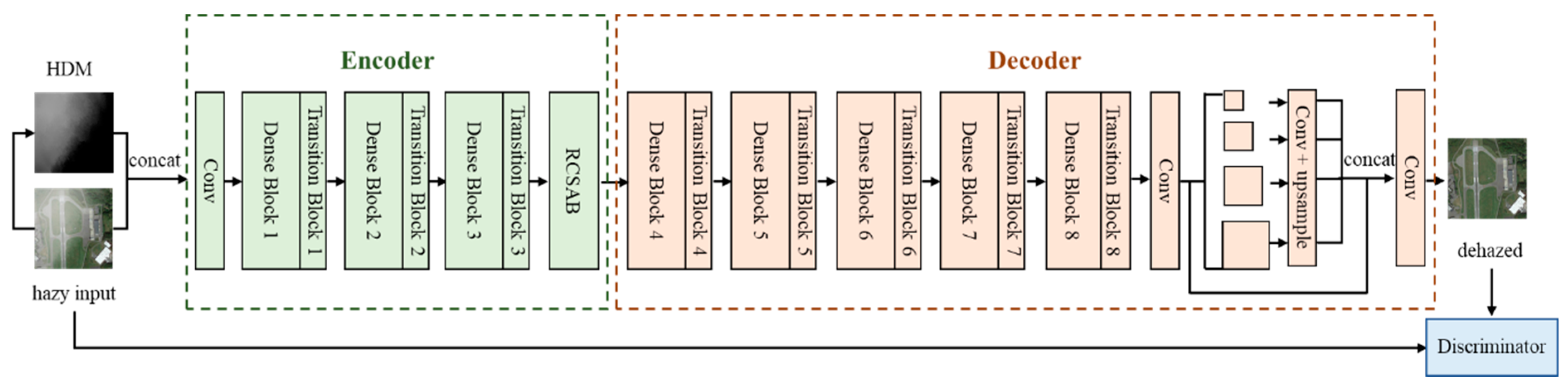
A single hazy remote sensing image dehazing solution, which combines both physical prior and deep learning technology, is presented to better describe the haze distribution in remote sensing images, and thus deal with non-uniform haze removal. In this solution, we first extract an HDM from the original hazy image, and subsequently leverage the HDM prior as input of the network together with the original hazy image.
(2)
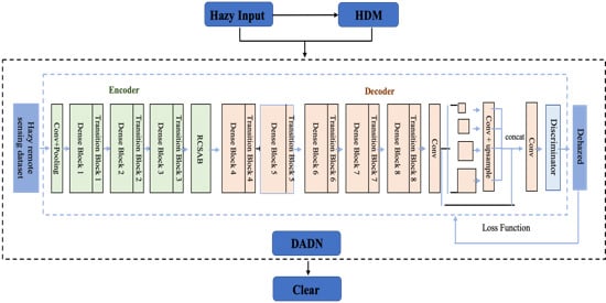
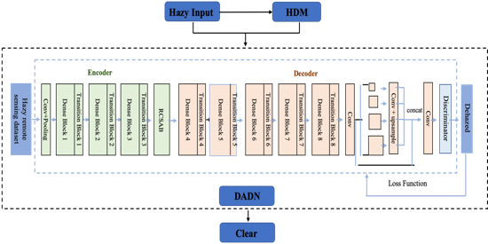
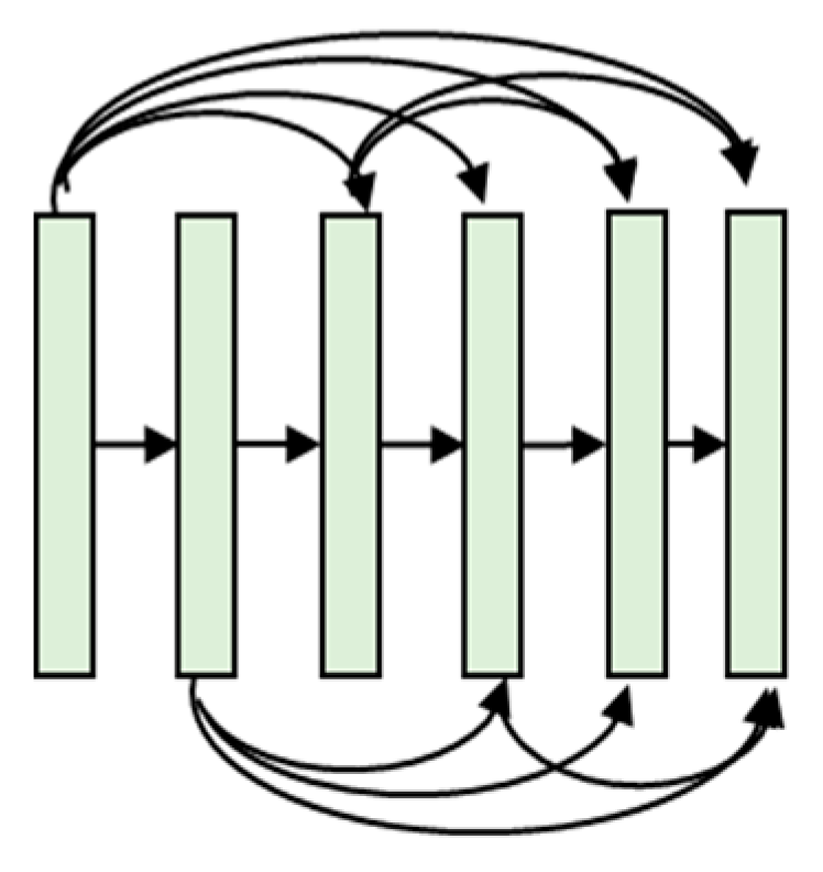
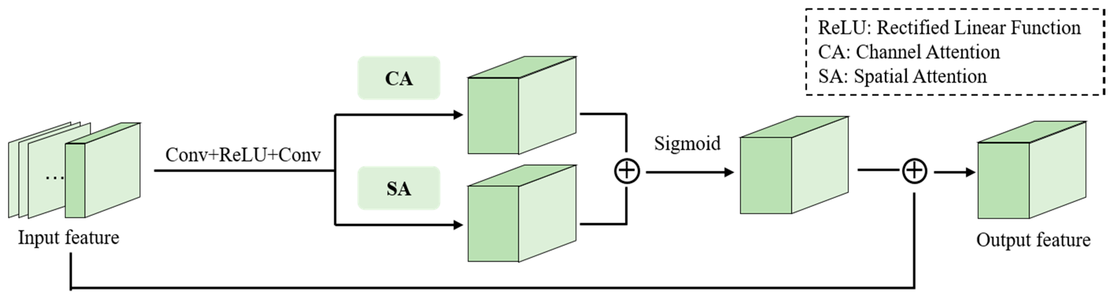
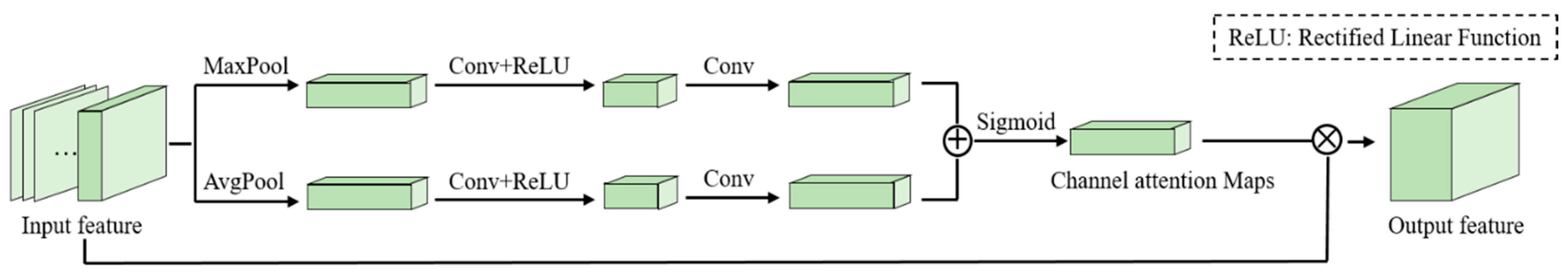
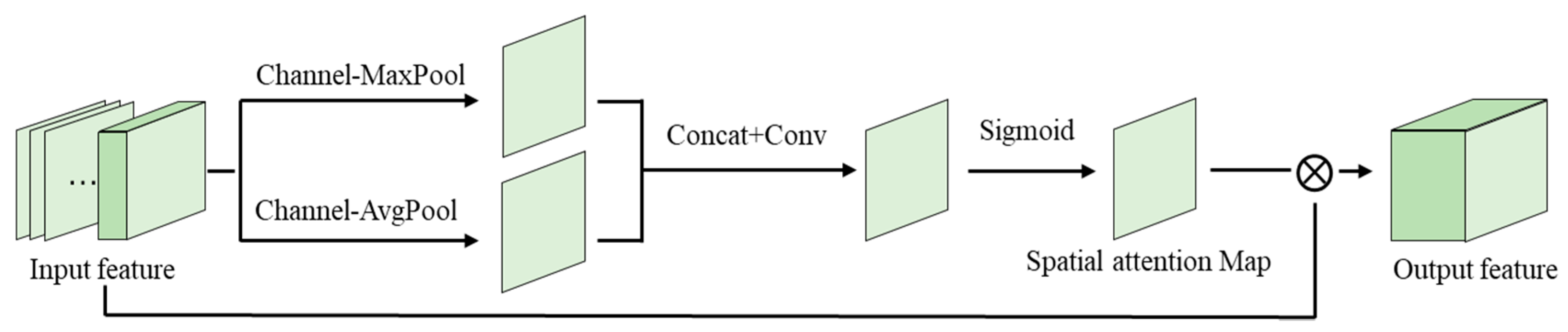
An encoder-decoder structured dehazing framework is proposed to directly learn clear images from input images, without estimation of any intermediate parameters. The proposed network is constructed based on dense blocks and attention blocks for accurate clear image estimation. Furthermore, we leverage a discriminator at the end of net to fine-tune the output and ensure that the estimated dehazed result is undifferentiated from the corresponding clear image.
(3)
A large-scale hazy remote sensing dataset is created as a benchmark which contains both uniform and non-uniform, high-resolution and low-resolution, synthetic and real hazy remote sensing images. Experimental results on the proposed dataset demonstrate the outstanding performance of the proposed method.
The remainder of the paper is organized as follows. Section 2 describes the degradation procedure caused by haze, as well as the details of the proposed dense attentive dehazing network (DADN). The experimental settings, results, and analysis are presented in Section 3 and a further discussion is presented in Section 4. Finally, our conclusions are given in Section 5.

2. Methodology

2.1. Atmospheric Scattering Model (ASM)

The image degradation caused by the presence of fog and haze is formulated mathematically by the ASM [11,28,29] as:
I ( x ) = J ( x ) t ( x ) + A ( 1 t ( x ) )
In this equation, J ( x ) and I ( x ) respectively denote the true scene radiance and the observed hazy image; A denotes the global atmospheric light, indicating the ambient light intensity; t ( x ) is the transmission matrix, which indicates the proportion of light which successfully arrives the sensor; and x is the pixel location. When A is uniform, the transmission matrix t ( x ) can be expressed as:
t ( x ) = e β d ( x )
where d ( x ) and β denote the depth of field and the extinction coefficient of the atmosphere, respectively. To obtain a clear image J ( x ) as output, we rewrite the model in Equation (1) as:
J ( x ) = 1 t ( x ) I ( x ) A 1 t ( x ) + A
According to the classical ASM, a similar three-step methodology is adopted in most of the existing single-image dehazing solutions as follows: (1) estimate the transmission map t ( x ) from the original hazy image I ( x ) ; (2) estimate the atmospheric light A using some other method (often empirical); (3) compute the clean image J ( x ) via Equation (3). Despite being intuitive and physically grounded, this three-step methodology transforms the problem of clear image lossy reconstruction directly into an estimation problem for parameters t ( x ) and A , giving rise to a suboptimal image restoration quality. To deal with this problem, we develop an encoder-decoder dehazing framework which directly learns the clear haze-free image from the original hazy image, enabling the network to measure the distortion of the clear image directly.

2.2. Network Architecture

Figure 1 presents the overall structure of the proposed DADN. Inspired by the successes of numerous computer vision tasks using dense networks [30,31] and attention mechanisms [32,33], we carefully designed the network in an encoder-decoder structure with dense blocks and attention blocks.
Specialized designed for single remote sensing image dehazing, where non-uniform haze is the most common state of haze, we came up with a solution to combine a haze density prior with deep learning to better describe haze distribution. In this solution, we first extract an initial HDM from the original hazy image, which can be regarded as a haze density prior, and subsequently use it as the input of the network, as well as the original hazy image. Furthermore, our network contains a discriminator at the end to fine-tune the dehazed output and ensure the estimated dehazed result is undifferentiated from the corresponding clear haze-free image.

2.2.1. Haze Density Map (HDM)

For remote sensing images, the depth of field d ( x ) in Equation (2) can be regarded as a constant since the distance between sensor and scene is always very large, and thus the haze intensity is mostly affected by the extinction coefficient β , which depends on the atmospheric conditions, and is rather unpredictable. Meanwhile, for a single regular close-range image, the extinction coefficient β can be regarded as a constant since the distance is limited, and thus the haze intensity is mostly affected by the depth of field, which is much easier to represent. We can see the comparison on close-range hazy images and remote sensing hazy images in the first two rows of Figure 2 where haze on the remote sensing images are much more irregularly distributed. Therefore, the haze intensity in remote sensing images is much more difficult to describe. To deal with this issue, we came up with a solution, i.e., combine a haze density prior with deep learning. Firstly, we extract a raw HDM from the original input hazy image. According to the assumption developed by Pan et al. in [34] that for hazy regions in a given image, the minimal intensity value is higher than the intensity value in haze-free regions, we extract the minimal intensity among the R, G, B channels to roughly describe the distribution of haze in the original hazy image. Thus, the raw HDM is defined as:
H r a w ( x ) = min c ( r , g , b ) I n c ( x )
where we normalize the hazy image I to [ 0 , 1 ] , represented as I n . The saturation S ( x ) , which indicates the purity of the color, is further utilized to make the HDM more precise since in a haze-free region the saturation will be higher than the saturation in a hazy region. Therefore, the modified HDM is expressed as:
H m o d i ( x ) = m a x ( H r a w ( x ) α S ( x ) , 0 )
S ( x ) = 1 3 m i n ( R ( x ) , G ( x ) , B ( x ) ) R ( x ) + G ( x ) + B ( x )
where α acts as an adjusted factor which controls how dark the haze-free regions will be and is empirically set as 2 in this paper to ensure that the haze-free region is gloomy enough; R, G, B, respectively represent the three color channels. Meanwhile, morphological opening [35] and a guided filter [36] are applied to lighten the impact of the scene texture, since the extracted HDM might remain some scene texture which needs to be reduced. Finally, the HDMs are extracted as shown in the third row of Figure 2.
The extracted HDM, which is regarded as the haze density prior, is then fed into the developed network, together with the original hazy image, to help the network better extract the haze-relevant features that describe the haze distribution.

2.2.2. Encoder

The encoder which maps the original inputs to an intermediate feature map, is carefully constructed with dense blocks and attention blocks.
(1) Dense Block
To tackle the issue of vanishing gradients, Huang et al. [37] developed a densely connected network, according to the observation that if CNNs contain shorter connections between the front layers and back layers, they can be satisfactorily deeper and achieve much more effective training. The structure of a 6-layer dense block is presented in Figure 3. Every layer is connected with the other layers in the forward way in a dense block, to solve the issue of vanishing gradient and at the same time strengthen the feature propagation. Taking the advantages of dense blocks into account, we utilize dense blocks with different layers to construct our network.
(2) Attention Block
Enlightened by the success of the attention mechanism in various computer vision problems [32,33,38], our network contains a residual channel-spatial attention block (RCSAB) to recalibrate the extracted feature maps, making the whole network focus more on important features, and thus better describing the non-uniform haze distribution. The proposed RCSAB takes advantage of both channel attention bocks and spatial attention blocks, and carefully operates them in a parallel way. A residual block is further combined for better feature mining. The architecture of the RCSAB is presented in Figure 4.
The channel attention block leveraged in this network can be found in Figure 5. Channel attention focuses on finding out the most meaningful features among the input feature maps, since every channel of the feature maps can be regarded as a feature detector. For effective computation of the channel attention map, the input feature maps are squeezed on the spatial dimension utilizing average-pooling as well as max-pooling. Convolutions with a kernel size of 1 × 1 are performed after the pooling, and an element-wise addition is applied to combine the feature maps from the different pooling operations. Finally, we obtain the output feature maps by multiplying the channel attention maps with original input feature maps.
Differing from channel attention, spatial attention is utilized to find out which part of the given input is an informative part. The most informative part, which usually contains lots of vital information about the haze distribution, is then the focus in the further learning. For computing, max-pooling and average-pooling are performed along the channel axis. Features after the pooling operations are then concatenated to create a spatial attention map (see in Figure 6). Similarly, multiplication is implemented between the computed spatial attention map and the original input feature maps, to obtain the final output.
To better exploit the benefits of both blocks, we combine these output features by performing element-wise addition. Meanwhile, we further integrate the spatial attention and channel attention blocks with a residual block, only focusing on the residual part between the input and output for more effective feature extraction.
As presented in Figure 1, the encoder contains three dense blocks, the corresponding transition blocks for down-sampling, and the RCSAB. The three dense blocks have respectively 6, 12, and 24 layers. Details of each layer are provided in Table 1. The feature size after the transition blocks is 1/32 of the input size, and the RCSAB does not change the feature size.

2.2.3. Decoder

Similarly, the decoder is made up of five dense blocks and the corresponding transition blocks for up-sampling (Figure 1). To better integrate features at different sizes, a pyramid pooling block [39] is added at the end of decoder, where four pooling operations with different kernel sizes (1/32, 1/16, 1/8, 1/4) are utilized. The features after the pooling operation are unsampled to the original size and then combined with the input feature to generate the result. Details of these layers are provided in Table 2.

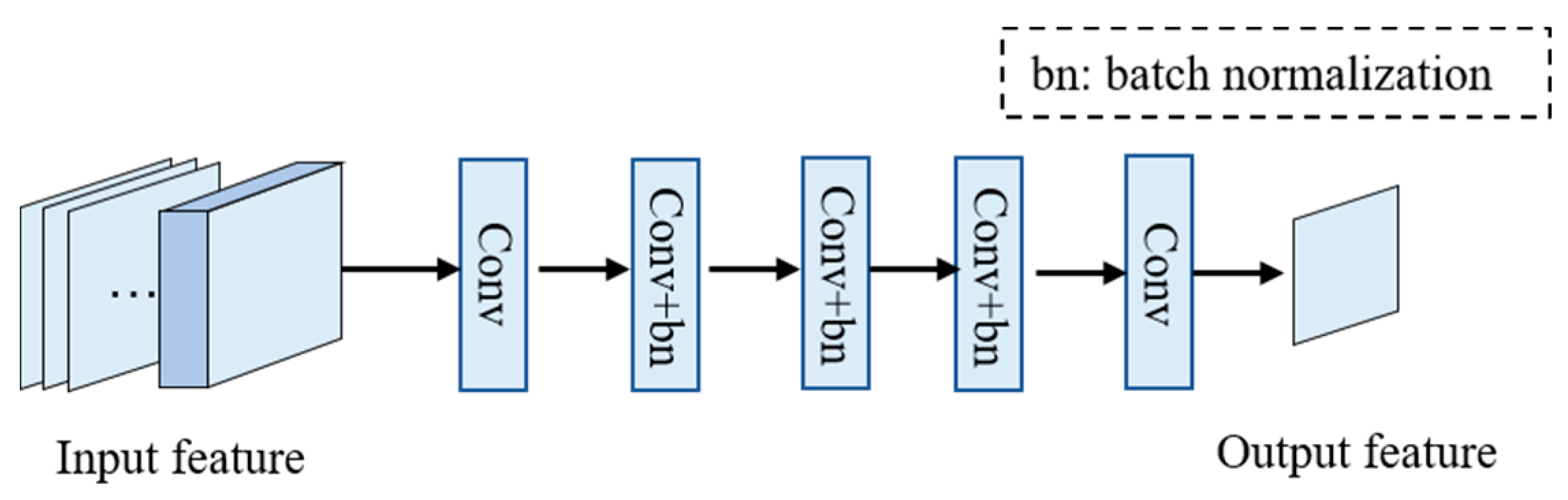
2.2.4. Discriminator

To make sure that the estimated dehazed result is almost undifferentiated from the corresponding clear image, a discriminator block is applied at the end of the net, where the above-mentioned encoder-decoder architecture can be regarded as a generator network. In our discriminator, several convolutions with kernel size 4 × 4 are performed. Given a 512 × 512 size input image, the output image size is 62 × 62. The discriminator structure is shown in Figure 7 and details are provided in Table 3.

2.3. Loss Function

For the discriminator, we train it to maximize the probability to assign the correct label (0 or 1) for the training dataset. The loss function for the proposed discriminator can be defined as [40]:
L D = E x _ r e a l ( l o g ( D ( x _ r e a l ) ) ) + E x _ f a k e ( l o g ( 1 D ( G ( x _ f a k e ) ) ) )
where D ( x ) denotes the discriminator’s estimation of the probability that real data instance x _ r e a l is real, E x _ r e a l is the expected value over all real data instances, G ( x _ f a k e ) is the generator’s output when given noise x _ f a k e , D ( G ( x _ f a k e ) ) denotes the discriminator’s estimation of the probability that a fake instance is real, and E x _ f a k e is the expected value over all generated fake instances G ( x _ f a k e ) . For the front encoder-decoder generator architecture, the loss function is composed of the edge-preserving loss function and generator loss:
L = L E + λ G L G
where the generator loss is expressed as:
L G = l o g ( 1 D ( G ( I ) )
The edge-preserving loss function was developed by Zhang et al. [19] to tackle the common problem of halo artifacts existing in the L 2 loss function, and contains three components: L 2 loss, gradient loss (both horizontal and vertical), and feature edge loss, which can be defined as:
L E = λ 1 L 2 + λ 2 L g r a + λ 3 L f e a
where L E is the edge-preserving loss, L g r a denotes the gradient loss, and L f e a indicates the feature edge loss. The two-directional gradient loss L g r a is defined as:
L g r a = G x ( F ( I ) ) G x ( J ) 2 + G y ( F ( I ) ) G y ( J ) 2
where G is the encoder-decoder network structure, I denotes the input hazy image, and J indicates the target clear image. G x and G y represent the gradient computing horizontally and vertically, respectively. The L f e a is expressed as:
L f e a = N 1 ( F ( I ) ) N 1 ( J ) 2 + N 2 ( F ( I ) ) N 2 ( J ) 2
where N i represents a CNN architecture. In this paper, the layers before relu1-1 and relu2-2 of VGG-16 [41] are utilized as N 1 and N 2 , respectively.
In summary, the proposed network adopts an encoder-decoder structure and is comprised of dense blocks and attention blocks. Considering the non-uniform haze distribution in remote sensing imagery, we came up with a solution to first extract an initial HDM from the original hazy image, which can be regard as the haze density prior, and use it as the input of the network, as well as the original hazy image. Furthermore, our network contains a discriminator at the end to fine-tune the dehazed result and guarantee that the final estimated result is undifferentiated from the corresponding clear image. For the loss function, we combine edge-preserving loss and generator loss. The network parameters are then achieved through minimizing the utilized loss function.

3. Experiments and Discussion

3.1. Experimental Settings

3.1.1. Datasets

A large-scale hazy remote sensing image dataset is created for this experiment. Since it is impractical to obtain paired haze-free and hazy remote sensing images of the same view and the same scene at the same time, synthetic hazy images were used for the network training. We synthesized both uniform and non-uniform hazy remote sensing image pairs as the training dataset, which contained a total of 13,980 images (12,000 for training and 1980 for validation) derived from the Aerial Image Dataset (AID) developed by Xia et al. [42], which was originally developed for aerial scene classification.
For generation of uniform hazy images, we set the atmospheric light A for a single image uniformly between [ 0.5 , 1 ] , and selected t { 0.4 , 0.6 } . The uniform hazy image was then generated through Equation (1), using clear images from the AID dataset. In this experiment, 720 uniform hazy remote sensing images were developed with a size of 512 × 512. For the non-uniform hazy images, we extracted 19 different transmission maps from real non-uniform remote sensing images using the method proposed by Pan et al. [34] and added them to the clear images from the AID dataset, thus generating, in total, 8940 non-uniform hazy images with a size of 512 × 512. Moreover, we added the generated uniform transmission maps and non-uniform transmission maps together to imitate more complex environments, so that another 4320 hazy images with size of 512 × 512 were developed. Therefore, a hazy remote sensing image dataset with a total of 13,980 image pairs (hazy image and corresponding clear image) was developed, containing both uniform and non-uniform hazy remote sensing images.
As for the test datasets, we constructed four kinds of dataset, containing both uniform and non-uniform, high-resolution and low-resolution, synthetic and real hazy remote sensing images, as listed below:
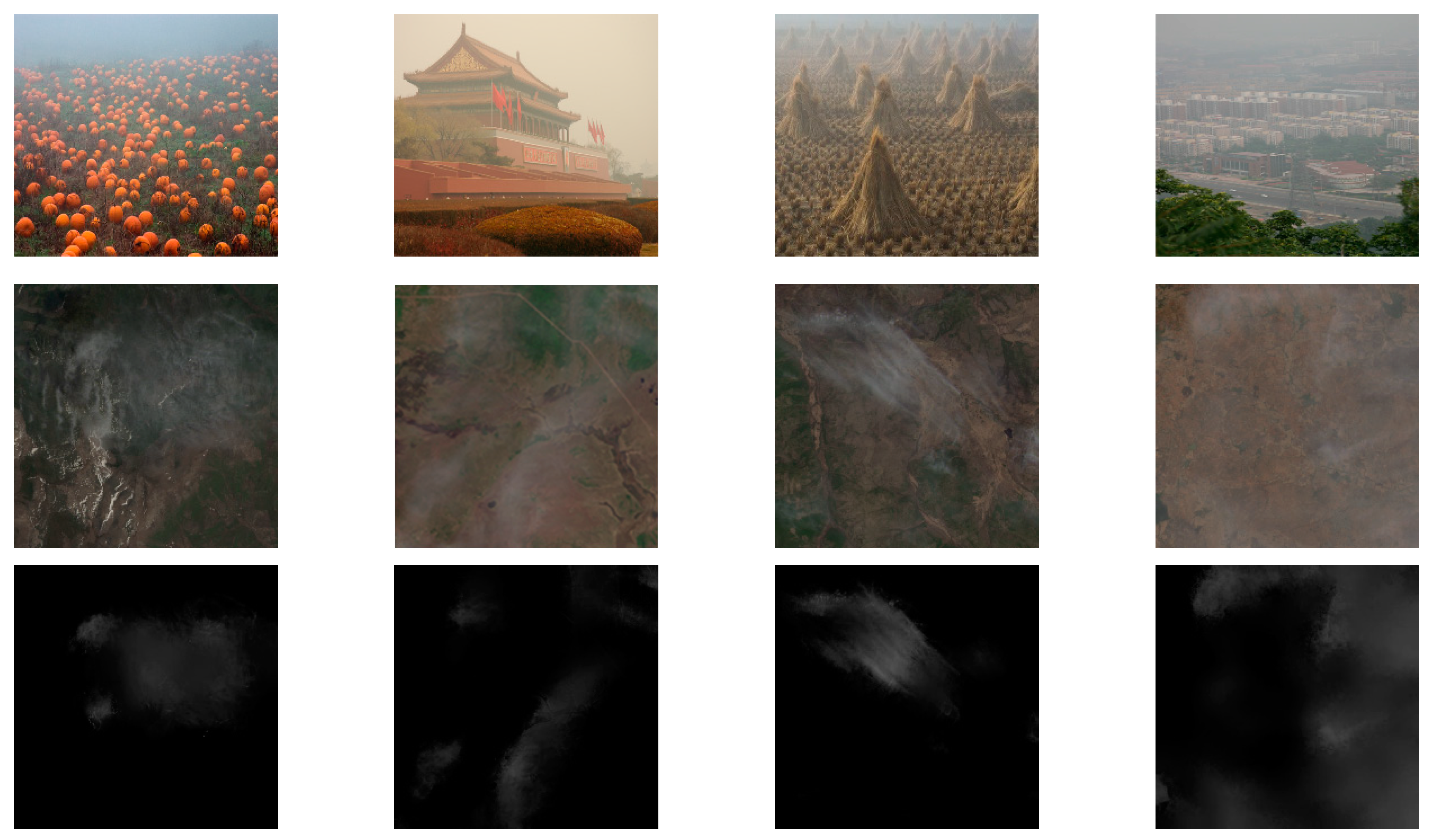
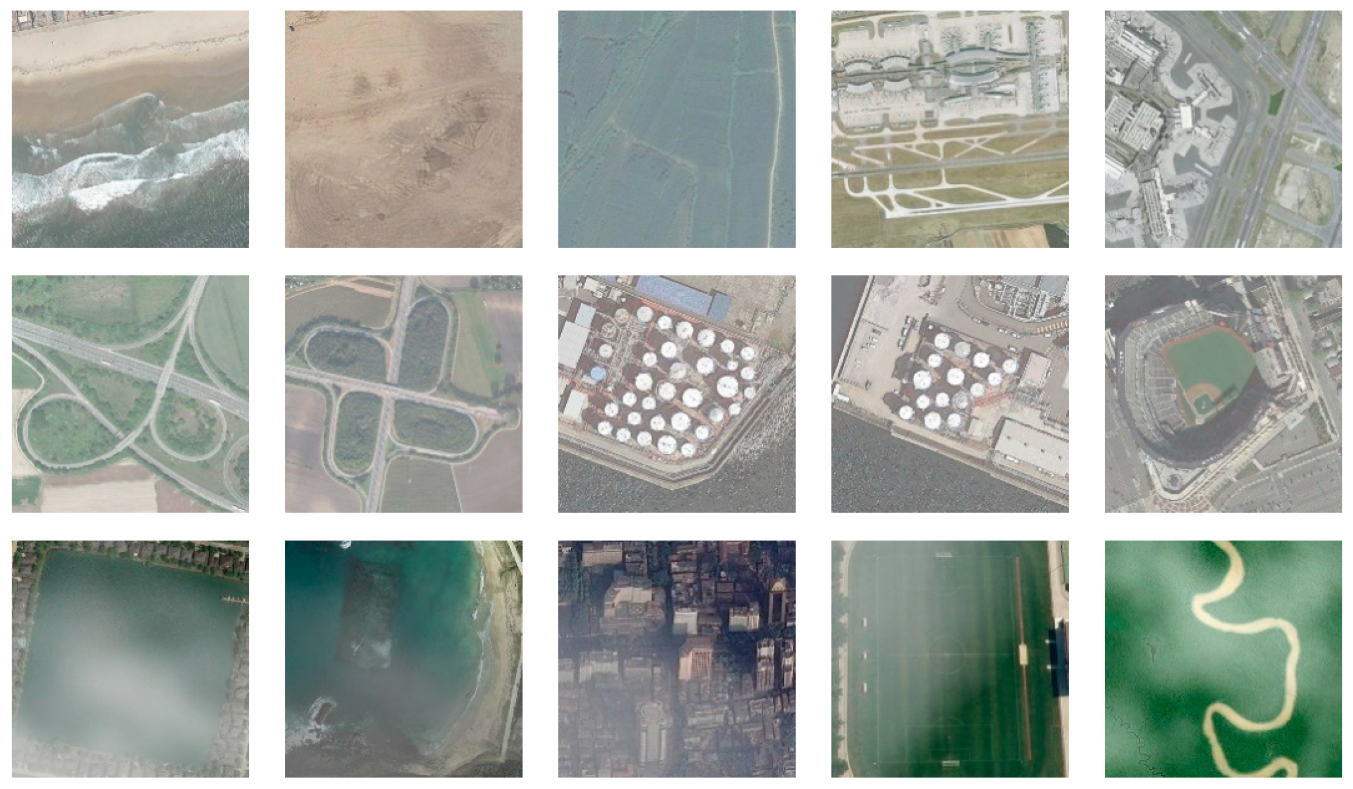
  • Test Dataset 1: Test dataset 1 consisted of 1650 synthetic uniform hazy remote sensing images. We simulated the images through the classical ASM Equation (1), with the rest of the AID dataset (1650 in total) as the clear images and t { 0.4 , 0.5 , 0.6 , 0.7 } (see examples in the first two rows of Figure 8).
  • Test Dataset 2: Test dataset 2 contained 1650 synthetic non-uniform hazy remote sensing images. With the non-uniform transition maps extracted from the real hazy images, we added these non-uniform transition maps to the clear images and created 1650 non-uniform hazy remote sensing images (see examples in the second two rows of Figure 8).
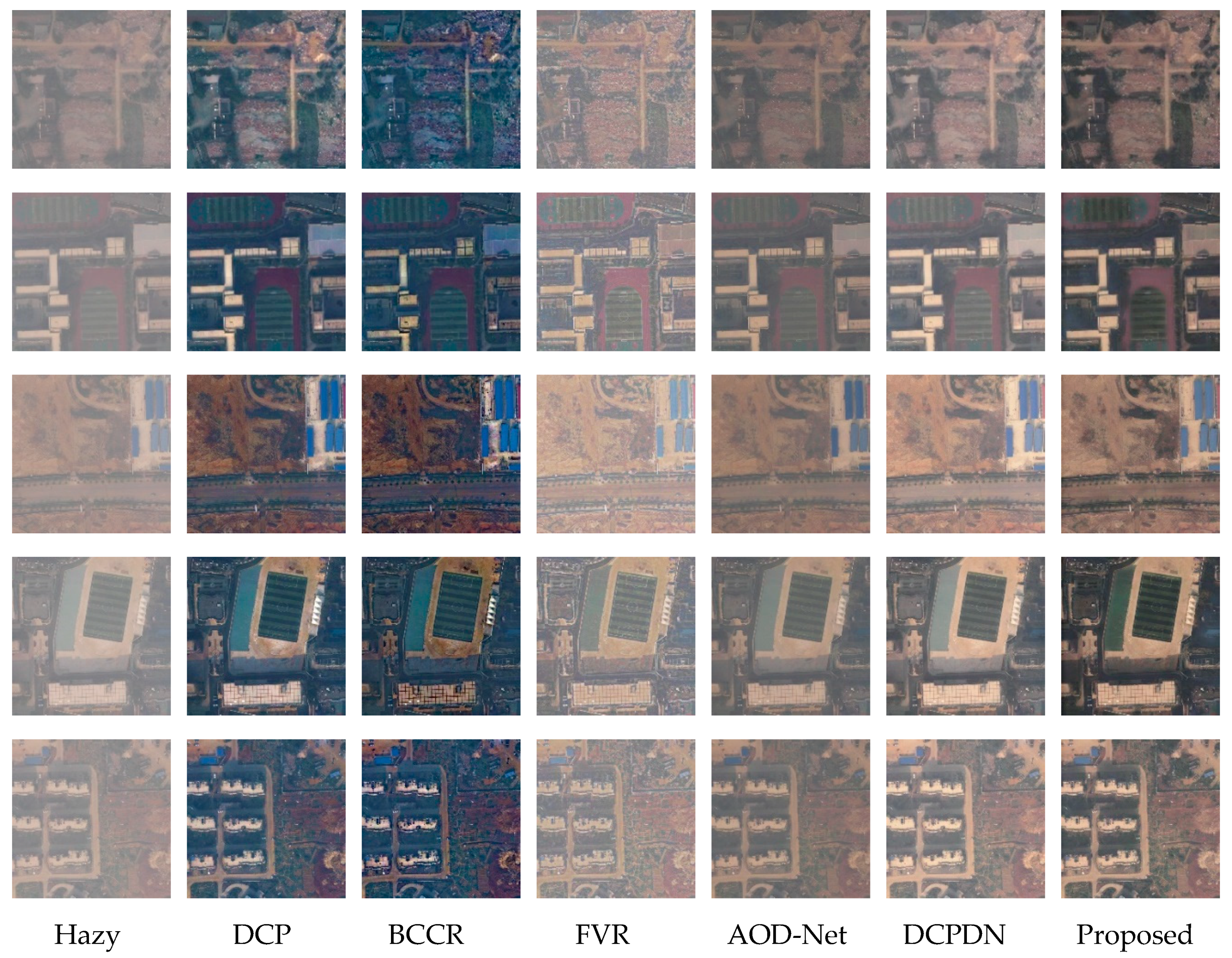
  • Test Dataset 3: Test dataset 3 was made up of real unmanned aerial vehicle (UAV) images obtained in August 2017 in Daye, China, under hazy weather conditions (see examples in the third two rows of Figure 8).
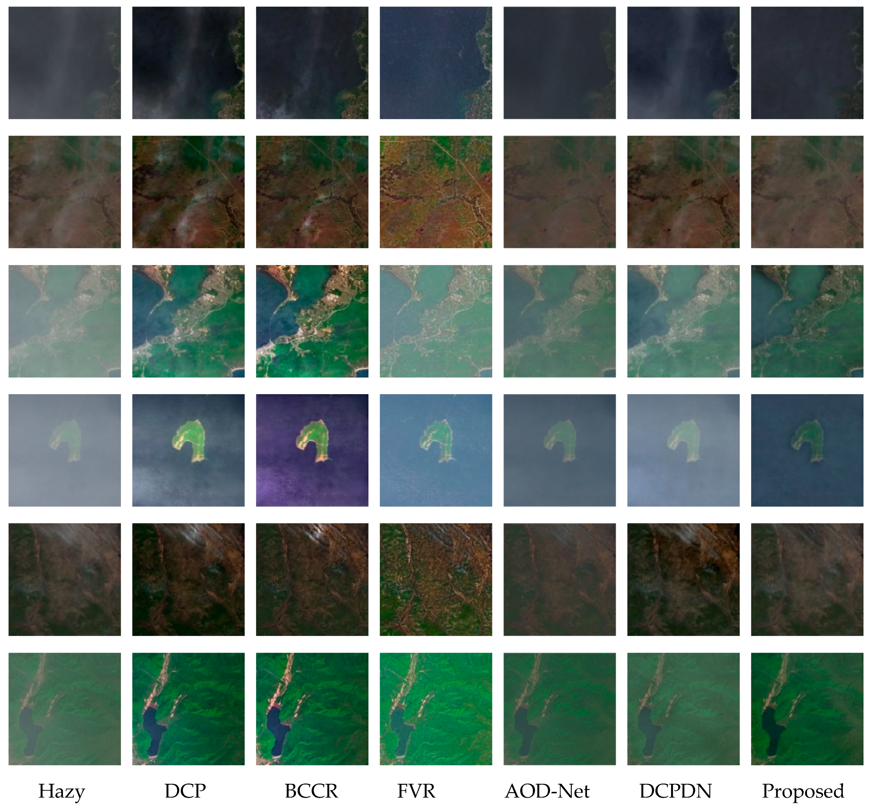
  • Test Dataset 4: Test dataset 4 consisted of real hazy remote sensing images from the Landsat 8 Operational Land Imager making use of the bands (2), (3), and (4) as BGR true color, (see examples in the last two rows of Figure 8).

3.1.2. Training Details

We used the PyTorch [43] framework for the training and testing. The model was trained with an NVIDIA RTX 2080 Ti GPU. ADAM [44] was leveraged as the optimization algorithm, with a batch size of 1. Meanwhile, we chose λ 1 = 1 , λ 2 = 0.5 , λ 3 = 0.8 , for the edge-preserving loss and λ G = 0.25 for the generator loss.

3.1.3. Evaluation Criteria

We utilize the full-reference criteria of the peak signal-to-noise ratio (PSNR) and structural similarity index (SSIM) to evaluate the dehazing results. For a single dehazed image, a higher PSNR value denotes higher similarity in pixel-wise values between the reference image and the result, and a higher SSIM value denotes that in terms of structural properties the dehazed result is much closer to the reference image.

3.2. Experimental Results

In this section, the experimental results obtained with both synthetic hazy remote sensing images and real-world hazy remote sensing images are presented. We compare the proposed solution with five prevailing methods of DCP [12], BCCR [13], Fast visibility restoration (FVR) [45], All-in-one Dehazing Network (AOD-Net) [18], and DCPDN [19].

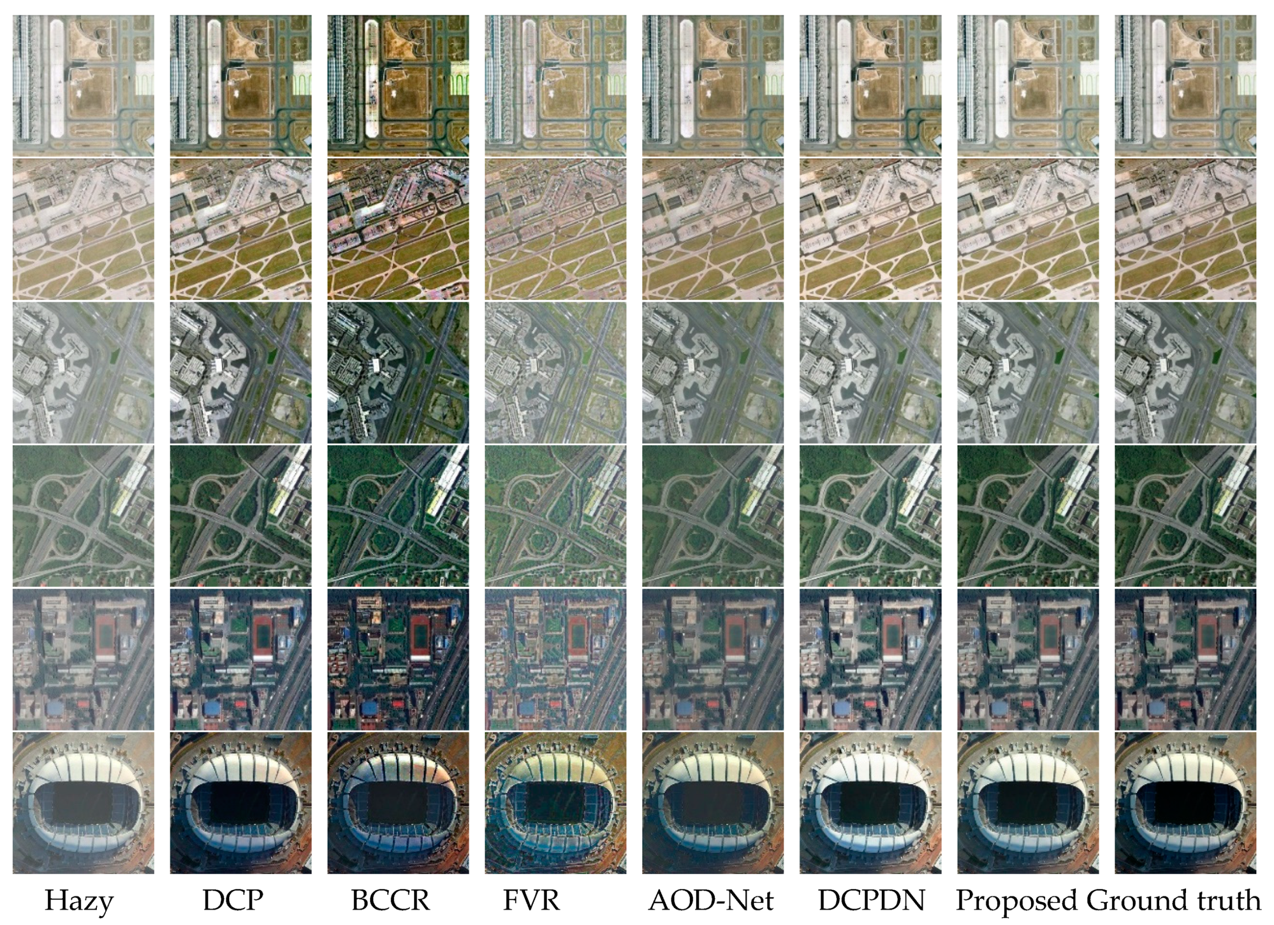
3.2.1. Results on Test Dataset 1

The results obtained with the synthetic uniform dataset are shown in Figure 9. The first column presents the synthetic hazy remote sensing images, the last column presents the ground truth images, and the other columns are the dehazed results of the different methods. DCP successfully removes most of the haze but tends to over-enhance the images, especially for the large white areas, since the DCP prior fails when color of the object is close to the atmospheric light. BCCR reveals the same problem of over-enhancement and leads to some color distortion (see the first two images), which is mainly due to the underestimation of the transmission matrices. The results of DCP and BCCR indicate the disadvantages of the prior-based methods, in that they can only obtain an accurate estimation when their assumptions fit perfectly. Since these priors are statistically achieved based on natural images, when it comes to remote sensing images, they may not fit and can lead to unsatisfactory dehazing results. FVR retains much of the haze and leads to obvious color distortions and artifacts, at the cost of saving time. The results of AOD-Net are not clear enough and tend to become dimmer than the ground truth. DCPDN achieves much more pleasing results for this uniform hazy dataset. However, unlike AOD-Net, DCPDN tends to lighten the dehazed results (see the last image), mainly caused by the inaccurate estimation of the atmospheric light. In contrast, the developed method, which avoids the estimation of intermediate parameters (transmission and atmospheric light) and directly measures the distortion of the clear image rather than that of the intermediate parameters, obtains the most pleasing results, with color and structural details that are the closest to the true haze-free images, verifying the advantage of the proposed network structure.
The PSNR and SSIM results are listed in Table 4. In accordance with the visual results, the developed method exceeds the other five methods, which demonstrates the outstanding performance of the proposed solution on uniform hazy remote sensing images.

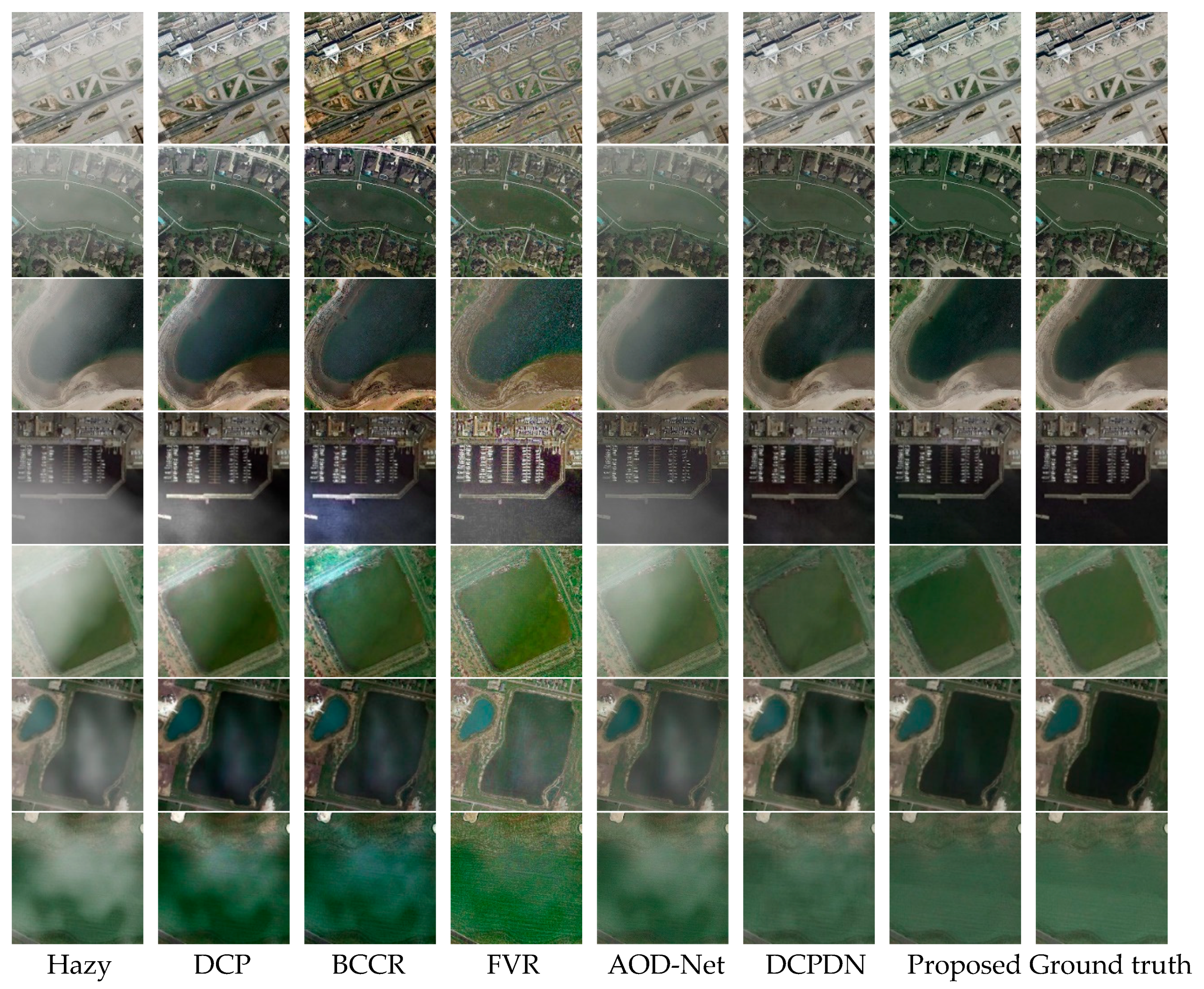
3.2.2. Results on Test Dataset 2

The results obtained with the synthetic non-uniform hazy remote sensing images using the developed method and the other prevailing methods are presented in Figure 10. Similarly, BBCR and DCP tend to over-enhance the results. Meanwhile, when dealing with large-scale non-uniform haze (see the last four hazy images), both DCP and BCCR fail to detect and handle the haze of different intensities, achieving rather unsatisfactory results, which indicates that these prior-based methods are limited when faced with non-uniform remote sensing images. FVR introduces serious color distortions and artifacts and cannot remove all the haze, but it appears to be not that sensitive to non-uniform haze, and thus achieves a better performance when dealing with this non-uniform dataset. The deep learning based AOD-Net and DCPDN are clearly sensitive to the non-uniform haze distribution, and retain obvious vestiges of non-uniform haze in their dehazed results (see the last five images), indicating that detecting and removing non-uniform haze from a single remote sensing image may be a rather difficult task for these deep learning-based methods, if there is not any additional prior information. By contrast, the developed method, benefiting from the HDM prior, successfully removes all the non-uniform haze and achieves results that are the closest to the truth clear images.
Similarly, we utilize PSNR and SSIM to evaluate the dehazing results (see Table 5). The table illustrates that the developed method obtains the highest PSNR and SSIM values, outperforming the other five methods and achieving the best dehazing results, which is in accordance with the quantitative analysis.
Overall, the proposed method deals with both uniform and non-uniform hazy images successfully and achieves the most visually pleasing dehazed results, without color distortions or artifacts.

3.2.3. Results on Test Dataset 3

The dehazing results obtained with the real hazy UAV images are shown in Figure 11. DCP and BCCR successfully remove most of the haze, but tend to over-enhance the image and lead to some color shift. FVR retains much of the haze in the result images, and introduces obvious color distortions and artifacts. AOD-Net and DCPDN again fail to remove all the haze, while the developed solution, with high contrast, vivid color, clear structure, and plausible results, obtains the most pleasing visual results, which demonstrate the effectiveness of the proposed method.

3.2.4. Results on Test Dataset 4
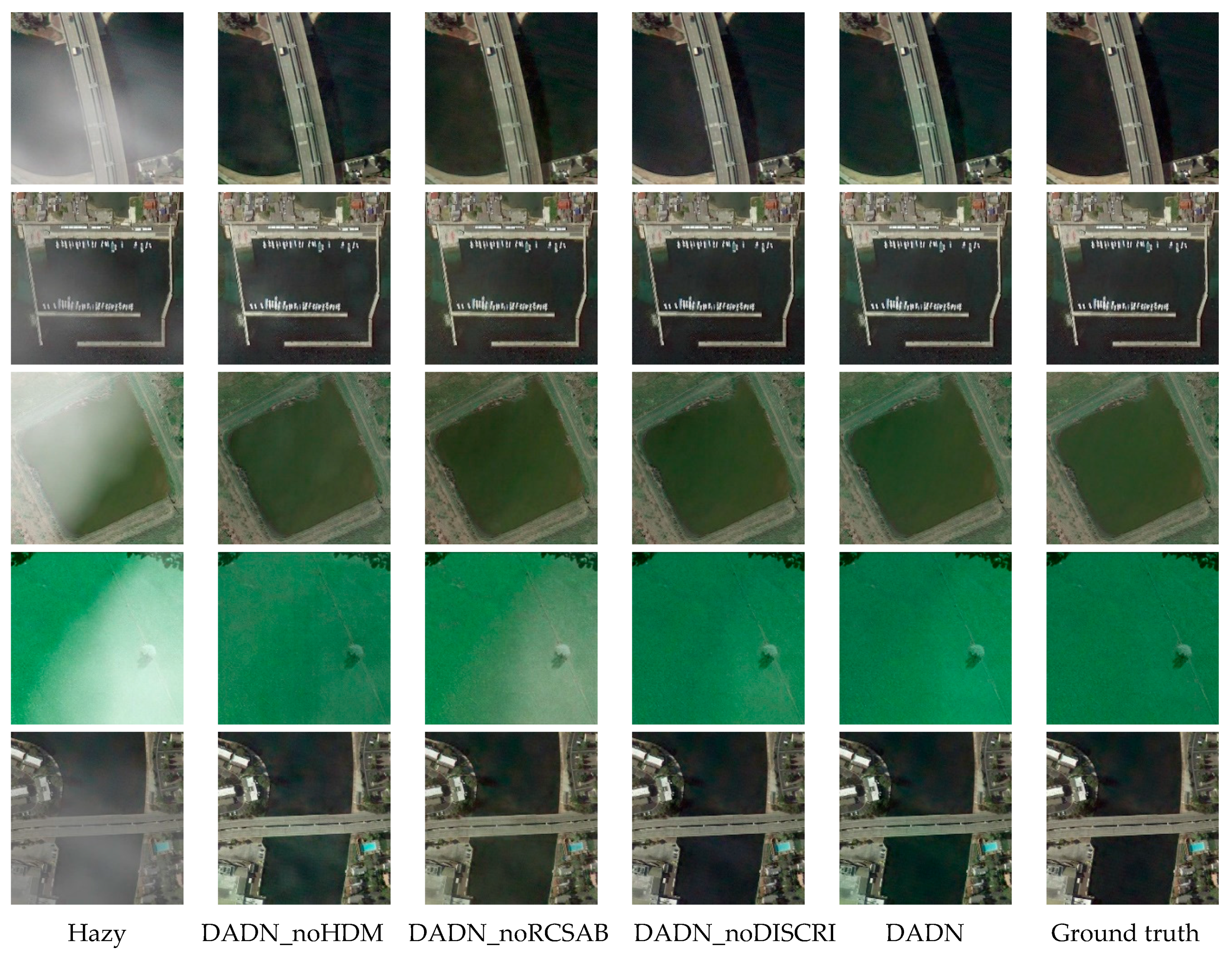
The results obtained with the second real hazy dataset of Landsat 8 OLI images are shown in Figure 12. As can be found, DCP and BCCR are sensitive to the non-uniform haze, and obvious traces of the non-uniform haze can still be seen. BCCR leads to obvious color distortion (especially the fourth image) and tends to over-enhance the image. The results of FVR do not retain many traces of non-uniform haze, indicating that FVR is not that sensitive to non-uniform haze, but it cannot remove all the haze, and introduces serious artifacts and color distortions. AOD-Net and DCPDN fail to remove all the haze, with much non-uniform haze remaining. In contrast, the proposed method removes most of the haze successfully, and there are very few traces of haze remaining in the results. Overall, the proposed method, which avoids estimating the transmission matrices and atmospheric light, with the help of the HDM prior, performs better than the other five methods when handling non-uniform haze in remote sensing images.

4. Discussion

In this study, we proposed a dense attentive dehazing network (DADN) which combines physical prior and deep learning technology to learn the mapping between the original input images and the corresponding haze-free image directly. Specialized designed for single remote sensing image dehazing, we propose to first extract an HDM from the original hazy image, which can be regarded as a haze density prior, and subsequently combine the HDM with the original hazy image as input of the network for a better description of the non-uniform haze distribution in hazy remote sensing images. Meanwhile, both spatial and channel attention blocks are carefully constructed in the network to recalibrate the extracted feature maps, thus allowing more adaptive and efficient training. To make sure that the estimated dehazed result is undifferentiated from the corresponding clear image, we further utilize a discriminator at the end of net, to refine the output.
To further validate the effectiveness of each module of the network, we conducted experiments on a network without the HDM (DADN_noHDM), a network without the discriminator (DADN_noDISCRI), and a network without the attention blocks (DADN_noRCSAB). The results are presented in Figure 13 and Table 6. DADN_noHDM and DADN_noRCSAB fail to detect the non-uniform haze, and obvious vestiges of haze remain, especially in the last two images, indicating that models without the HDM prior and RCSAB lack the ability to mine high-level haze-relevant features, and thus fail to remove all the non-uniform haze. Meanwhile, for the PSNR and SSIM criterion in Table 6, the proposed DADN method considerably outperforms DADN_noHDM and DADN_noRCSAB, which demonstrates that the haze density prior of the HDM and the attention module (RCSAB) are important and effective in the detection and removal of the non-uniform haze existing in remote sensing images. For the visual effects, DADN_noDISCRI and DADN are the most competitive methods, with vivid color, clear structure, and most of the non-uniform haze removed, while for the qualitative results, DADN outperforms DADN_noDISCRI, with the PSNR improved by 0.5. The qualitative results on the large-scale test data further validate the effectiveness of the proposed discriminator. Furthermore, a comparison on average consuming time (per image) is conducted. As we can see, our module makes obvious improvement in dehazing performance only with the cost of less than 0.06 s increase in time (per image), which is acceptable.
Overall, all the modules, i.e., the HDM prior, RCSAB, and the discriminator, are effective and necessary for single remote sensing image haze removal.

5. Conclusions

In this paper, we proposed a specialized solution for single remote sensing image dehazing which combines the haze density prior with deep learning technology. In the solution, the haze density prior HDM is extracted from the original hazy image at the first step and subsequently used as input of the network together with the original hazy image. The effectiveness of the HDM input has been further demonstrated through comparative experiments. A dense attentive dehazing network (DADN) is also presented in the solution, which composed of dense blocks and attention blocks (both spatial attention and channel attention) and directly learns the mapping from the input images to the corresponding haze-free image. The whole network contains an encoder-decoder architecture and has a discriminator at the end of the network, to further refine the dehazed results.
A large-scale hazy remote sensing dataset was created as a benchmark, which contains both uniform and non-uniform, synthetic and real hazy remote sensing images. The experimental results on the created dataset demonstrated that DADN achieves better performances than the other prevailing dehazing algorithms, especially when it comes to a non-uniform haze distribution. However, when handling large-scale dense haze, the proposed method may be challenged. In our further work, we will attempt to improve the performance of DADN by incorporating more background prior knowledge, and further mine haze-relevant features to better handle the large-scale dense haze existing in single remote sensing images.

Author Contributions

Conceptualization, Z.G. and Q.Y.; methodology, Z.G. and Q.Y.; formal analysis, Z.G.; investigation, Z.G. and Q.Y.; writing—original draft preparation, Z.G.; writing—review and editing, Q.Y., Z.Z., and L.Y; supervision, Q.Y., Z.Z., and L.Y. All authors read and approved the final manuscript.

Funding

This research is financially supported by the National Natural Science Foundation of China 41922008, 61971319 and 61871295.

Acknowledgments

This work was supported by the National Natural Science Foundation of China (No. 41922008, No. 61971319).

Conflicts of Interest

The authors declare no conflict of interest.

References

  1. Govender, M.; Chetty, K.; Bulcock, H. A review of hyperspectral remote sensing and its application in vegetation and water resource studies. Water SA 2007, 33, 145–151. [Google Scholar] [CrossRef] [Green Version]
  2. Casson, B.; Delacourt, C.; Allemand, P. Contribution of multi-temporal remote sensing images to characterize landslide slip surface‒Application to the La Clapière landslide (France). Nat. Hazards Earth Syst. Sci. 2005, 5, 425–437. [Google Scholar] [CrossRef]
  3. Sobrino, J.A.; Raissouni, N. Toward remote sensing methods for land cover dynamic monitoring: Application to Morocco. Int. J. Remote Sens. 2000, 21, 353–366. [Google Scholar] [CrossRef]
  4. Valero, S.; Chanussot, J.; Benediktsson, J.A.; Talbot, H.; Waske, B. Advanced directional mathematical morphology for the detection of the road network in very high resolution remote sensing images. Pattern Recognit. Lett. 2010, 31, 1120–1127. [Google Scholar] [CrossRef] [Green Version]
  5. Kopf, J.; Neubert, B.; Chen, B.; Cohen, M.; Cohen-Or, D.; Deussen, O.; Uyttendaele, M.; Lischinski, D. Deep Photo: Model-Based Photograph Enhancement and Viewing; ACM: New York, NY, USA, 2008. [Google Scholar]
  6. Narasimhan, S.G.; Nayar, S.K. Removing weather effects from monochrome images. In Proceedings of the IEEE computer society conference on computer vision and pattern recognition, Kauai, HI, USA, 8–14 December 2001; p. II. [Google Scholar]
  7. Schechner, Y.Y.; Narasimhan, S.G.; Nayar, S.K. Instant dehazing of images using polarization. In Proceedings of the 2001 IEEE Computer Society Conference on Computer Vision and Pattern Recognition. CVPR 2001, Kauai, HI, USA, 8–14 December 2001. [Google Scholar]
  8. Treibitz, T.; Schechner, Y.Y. Polarization: Beneficial for visibility enhancement. In Proceedings of the 2009 IEEE Conference on Computer Vision and Pattern Recognition, Miami, FL, USA, 20–25 June 2009; pp. 525–532. [Google Scholar]
  9. Xu, Z.; Liu, X.; Ji, N. Fog removal from color images using contrast limited adaptive histogram equalization. In Proceedings of the 2009 2nd International Congress on Image and Signal Processing, Tianjin, China, 17–19 October 2009; pp. 1–5. [Google Scholar]
  10. Narasimhan, S.G.; Nayar, S.K. Contrast restoration of weather degraded images. IEEE Trans. Pattern Anal. Mach. Intell. 2003, 25, 713–724. [Google Scholar] [CrossRef] [Green Version]
  11. McCartney, E.J. Optics of the Atmosphere: Scattering by Molecules and Particles; John Wiley and Sons, Inc.: New York, NY, USA, 1976; 421p. [Google Scholar]
  12. He, K.; Sun, J.; Tang, X. Single image haze removal using dark channel prior. IEEE Trans. Pattern Anal. Mach. Intell. 2011, 33, 2341–2353. [Google Scholar]
  13. Meng, G.; Wang, Y.; Duan, J.; Xiang, S.; Pan, C. Efficient image dehazing with boundary constraint and contextual regularization. In Proceedings of the 2013 IEEE International Conference on Computer Vision, Sydney, NSW, Australia, 1–8 December 2013; pp. 617–624. [Google Scholar]
  14. Zhu, Q.; Mai, J.; Shao, L. A fast single image haze removal algorithm using color attenuation prior. IEEE Trans. Image Process. 2015, 24, 3522–3533. [Google Scholar]
  15. Berman, D.; Avidan, S. Non-local image dehazing. In Proceedings of the IEEE Conference on Computer Vision and Pattern Recognition, Las Vegas, NV, USA, 27–30 June 2016; pp. 1674–1682. [Google Scholar]
  16. Cai, B.; Xu, X.; Jia, K.; Qing, C.; Tao, D. Dehazenet: An end-to-end system for single image haze removal. IEEE Trans. Image Process. 2016, 25, 5187–5198. [Google Scholar] [CrossRef] [Green Version]
  17. Ren, W.; Liu, S.; Zhang, H.; Pan, J.; Cao, X.; Ynag, M.-H. Single image dehazing via multi-scale convolutional neural networks. In Proceedings of the European Conference on Computer Vision, Amsterdam, The Netherlands, 8–16 October 2016; pp. 154–169. [Google Scholar]
  18. Li, B.; Peng, X.; Wang, Z.; Xu, J.; Feng, D. Aod-net: All-in-one dehazing network. In Proceedings of the IEEE International Conference on Computer Vision, Venice, Italy, 22–29 October 2017; pp. 4770–4778. [Google Scholar]
  19. Zhang, H.; Patel, V.M. Densely connected pyramid dehazing network. In Proceedings of the IEEE Conference on Computer Vision and Pattern Recognition, Salt Lake City, UT, USA, 18–22 June 2018; pp. 3194–3203. [Google Scholar]
  20. Fu, X.; Wang, J.; Zeng, D.; Huang, Y.; Ding, X. Remote sensing image enhancement using regularized-histogram equalization and DCT. IEEE Geosci. Remote Sens. Lett. 2015, 12, 2301–2305. [Google Scholar] [CrossRef]
  21. Makarau, A.; Richter, R.; Müller, R.; Reinartz, P. Haze detection and removal in remotely sensed multispectral imagery. IEEE Trans. Geosci. Remote Sens. 2014, 52, 5895–5905. [Google Scholar] [CrossRef] [Green Version]
  22. Long, J.; Shi, Z.; Tang, W.; Zhang, C. Single remote sensing image dehazing. IEEE Geosci. Remote Sens. Lett. 2014, 11, 59–63. [Google Scholar] [CrossRef]
  23. Shen, H.; Li, H.; Qian, Y.; Zhang, L.; Yuan, Q. An effective thin cloud removal procedure for visible remote sensing images. ISPRS J. Photogramm. Remote Sens. 2014, 96, 224–235. [Google Scholar] [CrossRef]
  24. Zhang, Y.; Guindon, B.; Cihlar, J. An image transform to characterize and compensate for spatial variations in thin cloud contamination of Landsat images. Remote Sens. Environ. 2002, 82, 173–187. [Google Scholar] [CrossRef]
  25. Jiang, H.; Lu, N.; Yao, L. A high-fidelity haze removal method based on hot for visible remote sensing images. Remote Sens. 2016, 8, 844. [Google Scholar] [CrossRef] [Green Version]
  26. Liu, Q.; Gao, X.; He, L.; Lu, W. Haze removal for a single visible remote sensing image. Signal Process. 2017, 137, 33–43. [Google Scholar] [CrossRef]
  27. Xie, F.; Chen, J.; Pan, X.; Jiang, Z. Adaptive Haze Removal for Single Remote Sensing Image. IEEE Access 2018, 6, 67982–67991. [Google Scholar] [CrossRef]
  28. Narasimhan, S.G.; Nayar, S.K. Chromatic framework for vision in bad weather. In Proceedings of the IEEE Conference on Computer Vision and Pattern Recognition, Hilton Head Island, SC, USA, 15 June 2000; Volume 1, pp. 598–605. [Google Scholar]
  29. Narasimhan, S.G.; Nayar, S.K. Vision and the atmosphere. Int. J. Comput. Vis. 2002, 48, 233–254. [Google Scholar] [CrossRef]
  30. Zhang, H.; Patel, V.M. Density-aware single image de-raining using a multi-stream dense network. In Proceedings of the IEEE Conference on Computer Vision and Pattern Recognition, Salt Lake City, UT, USA, 18–22 June 2018; pp. 695–704. [Google Scholar]
  31. Pelt, D.M.; Sethian, J.A. A mixed-scale dense convolutional neural network for image analysis. Proc. Natl. Acad. Sci. USA 2018, 115, 254–259. [Google Scholar] [CrossRef] [Green Version]
  32. Zhang, Y.; Li, K.; Li, K.; Wang, L.; Zhong, B.; Fu, Y. Image super-resolution using very deep residual channel attention networks. In Proceedings of the European Conference on Computer Vision (ECCV), Munich, Germany, 8–14 September 2018; pp. 286–301. [Google Scholar]
  33. Kim, J.H.; Choi, J.H.; Cheon, M.; Lee, J.-S. RAM: Residual Attention Module for Single Image Super-Resolution. arXiv 2018, arXiv:1811.12043. [Google Scholar]
  34. Pan, X.; Xie, F.; Jiang, Z.; Shi, Z.; Luo, X. No-reference assessment on haze for remote-sensing images. IEEE Geosci. Remote Sens. Lett. 2016, 13, 1855–1859. [Google Scholar] [CrossRef]
  35. Dougherty, E.R.; Lotufo, R.A. Hands-on Morphological Image Processing; SPIE Press: Bellingham, WA, USA, 2003. [Google Scholar]
  36. He, K.; Sun, J.; Tang, X. Guided image filtering. IEEE Trans. Pattern Anal. Mach. Intell. 2013, 35, 1397–1409. [Google Scholar] [CrossRef] [PubMed]
  37. Huang, G.; Liu, Z.; Van Der Maaten, L.; Weinberger, K.Q. Densely connected convolutional networks. In Proceedings of the IEEE Conference on Computer Vision and Pattern Recognition, Honolulu, HI, USA, 21–26 July 2017; pp. 4700–4708. [Google Scholar]
  38. Woo, S.; Park, J.; Lee, J.Y.; Kweon, I.S. Cbam: Convolutional block attention module. In Proceedings of the European Conference on Computer Vision, Munich, Germany, 8–14 September 2018; pp. 3–19. [Google Scholar]
  39. Lazebnik, S.; Schmid, C.; Ponce, J. Beyond bags of features: Spatial pyramid matching for recognizing natural scene categories. In Proceedings of the IEEE Computer Society Conference on Computer Vision and Pattern Recognition, New York, NY, USA, 17–22 June 2006; Volume 2, pp. 2169–2178. [Google Scholar]
  40. Goodfellow, I.; Pouget-Abadie, J.; Mirza, M.; Xu, B.; Warde-Farley, D.; Ozair, S.; Courville, A.; Bengio, Y. Generative adversarial nets. Adv. Neural Inf. Process. Syst. 2014, 2672–2680. [Google Scholar]
  41. Simonyan, K.; Zisserman, A. Very deep convolutional networks for large-scale image recognition. arXiv 2014, arXiv:1409.1556. [Google Scholar]
  42. Xia, G.-S.; Hu, J.; Hu, F.; Shi, B.; Bai, X.; Zhong, Y.; Zhang, L.; Lu, X. AID: A benchmark data set for performance evaluation of aerial scene classification. IEEE Trans. Geosci. Remote Sens. 2017, 55, 3965–3981. [Google Scholar] [CrossRef] [Green Version]
  43. Ketkar, N. Introduction to PyTorch. In Deep Learning with Python; Apress: Berkeley, CA, USA, 2017; pp. 195–208. [Google Scholar]
  44. Kingma, D.P.; Ba, J. Adam: A method for stochastic optimization. In Proceedings of the 3rd International Conference for Learning Representations, San Diego, CA, USA, 7–9 May 2015. [Google Scholar]
  45. Tarel, J.P.; Hautiere, N. Fast visibility restoration from a single color or gray level image. In Proceedings of the IEEE 12th International Conference on Computer Vision, Kyoto, Japan, 29 September–2 October 2009; pp. 2201–2208. [Google Scholar]
Figure 1. Overall architecture of the proposed dehazing network.
Remotesensing 11 03008 g001
Figure 2. Close-range hazy images (first row), remote sensing hazy images (second row), and their corresponding haze density maps (HDMs) (third row).
Remotesensing 11 03008 g002
Figure 3. Architecture of a 6-layer dense block.
Remotesensing 11 03008 g003
Figure 4. Architecture of the proposed residual channel-spatial attention block (RCSAB).
Remotesensing 11 03008 g004
Figure 5. Architecture of the channel attention block.
Remotesensing 11 03008 g005
Figure 6. Architecture of the spatial attention block.
Remotesensing 11 03008 g006
Figure 7. Architecture of the discriminator.
Remotesensing 11 03008 g007
Figure 8. Examples of the created hazy remote sensing dataset. (First two rows): synthetic uniform hazy images; (second two rows): synthetic non-uniform hazy images; (third two rows): real hazy unmanned aerial vehicle (UAV) images; (last two rows): real hazy Landsat images.
Remotesensing 11 03008 g008aRemotesensing 11 03008 g008b
Figure 9. Dehazed results on test dataset 1.
Remotesensing 11 03008 g009
Figure 10. Dehazed results on test dataset 2.
Remotesensing 11 03008 g010
Figure 11. Dehazed results on test dataset 3.
Remotesensing 11 03008 g011
Figure 12. Dehazed results on test dataset 4.
Remotesensing 11 03008 g012
Figure 13. Dehazed results for the test modules.
Remotesensing 11 03008 g013
Table 1. Details of the encoder.
LayerOperationOutput SizeOutput Channels
Input 512 × 5126
Convolution7 × 7 convolution, stride = 2256 × 25664
Pooling3 × 3 max pooling, stride = 2128 × 12864
Dense block 1 ( 1 × 1   convolution ,   3 × 3   convolution ) × 6 128 × 128256
Transition block 11 × 1 convolution, stride = 1128 × 128128
2 × 2 average pooling, stride = 264 × 64
Dense block 2   ( 1 × 1   convolution ,   3 × 3   convolution ) × 12 64 × 64512
Transition block 21 × 1 convolution, stride = 264 × 64256
2 × 2 average pooling, stride = 232 × 32
Dense block 3   ( 1 × 1   convolution ,   3 × 3   convolution ) × 24 32 × 321024
Transition block 31 × 1 convolution, stride = 232 × 32512
2 × 2 average pooling, stride = 216 × 16
RCSABConvolution   ( 3 × 3   convolution ) × 2 16 × 16512
Channel attention16 × 16 average pooling, 16 × 16 max pooling
Spatial attentionchannel average pooling, channel max pooling
Table 2. Details of the decoder.
LayerOperationOutput SizeOutput Channels
Dense block 41 × 1 convolution, 3 × 3 convolution16 × 16768
Transition block 41 × 1 convolution16 × 16384
nearest upsample, scale = 232 × 32
Dense block 51 × 1 convolution, 3 × 3 convolution32 × 32640
Transition block 51 × 1 convolution32 × 32256
nearest upsample, scale = 264 × 64
Dense block 61 × 1 convolution, 3 × 3 convolution64 × 64384
Transition block 61 × 1 convolution64 × 6464
nearest upsample, scale = 2128 × 128
Dense block 71 × 1 convolution, 3 × 3 convolution128 × 128128
Transition block 71 × 1 convolution128 × 12832
nearest upsample, scale = 2256 × 256
Dense block 81 × 1 convolution, 3 × 3 convolution256 × 25664
Transition block 81 × 1 convolution256 × 25616
nearest upsample, scale = 2512 × 512
Convolution3 × 3 convolution512 × 51220
Pyramid pooling block32 × 32 average pooling, 1 × 1 convolution, nearest upsample512 × 5121
16 × 16 average pooling, 1 × 1 convolution, nearest upsample512 × 5121
8 × 8 average pooling, 1 × 1 convolution, nearest upsample512 × 5121
4 × 4 average pooling, 1 × 1 convolution, nearest upsample512 × 5121
Convolution3 × 3 convolution512 × 5123
Dehazed output 512 × 5123
Table 3. Details of the discriminator.
LayerOperationOutput SizeOutput Channels
input 512 × 5123
Convolution4 × 4 convolution, stride = 2256 × 25664
Convolution4 × 4 convolution, stride = 2128 × 128128
Batch normalizationbatch normalization128 × 128128
Convolution4 × 4 convolution, stride = 264 × 64256
Batch normalizationbatch normalization64 × 64256
Convolution4 × 4 convolution, stride = 163 × 63512
Batch normalizationbatch normalization63 × 63512
Convolution4 × 4 convolution, stride = 162 × 621
Table 4. Quantitative results obtained with the synthetic uniform hazy remote sensing images (average of 1650 images).
DCPBCCRFVRAOD-NetDCPDNProposed
PSNR22.427020.157816.083322.726723.800231.5095
SSIM0.88530.784600.81090.91370.93970.9888
Table 5. Quantitative results obtained with the synthetic non-uniform hazy remote sensing images (average of 1650 images).
DCPBCCRFVRAOD-NetDCPDNProposed
PSNR19.934417.757616.135619.527528.073734.9841
SSIM0.81320.73990.47730.821330.88860.8990
Table 6. Quantitative results for the test modules.
DADN_noHDMDADN_noRCSABDADN_noDISCRIProposed
PSNR30.466829.369534.657535.1895
SSIM0.89190.88940.89640.8965
Time0.18410.22620.18910.2368

