Article

Multi-Temporal and Multi-Frequency SAR Analysis for Forest Land Cover Mapping of the Mai-Ndombe District (Democratic Republic of Congo)

by
Jörg Haarpaintner
1,* and
Heidi Hindberg
2
1
NORCE—Norwegian Research Centre AS, NORCE Climate, P.O. Box 6434, N-9294 Tromsø, Norway
2
NORCE—Norwegian Research Centre AS, NORCE Technology, P.O. Box 6434, N-9294 Tromsø, Norway
*
Author to whom correspondence should be addressed.
Remote Sens. 2019, 11(24), 2999; https://doi.org/10.3390/rs11242999
Submission received: 27 September 2019 / Revised: 5 December 2019 / Accepted: 10 December 2019 / Published: 13 December 2019
(This article belongs to the Special Issue Advances in Active Remote Sensing of Forests)

Abstract

:
The European Space Agency’s (ESA) “SAR for REDD” project aims to support complementing optical remote sensing capacities in Africa with synthetic aperture radar (SAR) for Reducing Emissions from Deforestation and Forest Degradation (REDD). The aim of this study is to assess and compare Sentinel-1 C-band, ALOS-2 PALSAR-2 L-band and combined C/L-band SAR-based land cover mapping over a large tropical area in the Democratic Republic of Congo (DRC). The overall approach is to benefit from multi-temporal observations acquired from 2015 to 2017 to extract statistical parameters and seasonality of backscatters to improve forest land cover (FLC) classification. We investigate whether and to what extent the denser time series of C- band SAR can compensate for the L-band’s deeper vegetation penetration depth and known better FLC mapping performance. The supervised classification differentiates into forest, inundated forest, woody savannah, dry and wet grassland, and river swamps. Several feature combinations of statistical parameters from both, single and multi-frequency observations in a multivariate maximum-likelihood classification are compared. The FLC maps are reclassified into forest, savannah, and grassland (FSG) and validated with a systematic sampling grid of manual interpretations of very-high-resolution optical satellite data. Using the temporal variability of the dual-polarized backscatters, in the form of either wet/dry seasonal averages or using the statistical variance, in addition to the average backscatter, increased the classification accuracies by 4–5 percent points and 1–2 percent points for C- and L-band, respectively. For the FSG validation overall accuracies of 84.4%, 89.1%, and 90.0% were achieved for single frequency C- and L-band, and C/L-band combined, respectively. The resulting forest/non-forest (FNF) maps with accuracies of 90.3%, 92.2%, and 93.3%, respectively, are then compared to the Landsat-based Global Forest Change program’s and JAXA’s ALOS-1/2 based global FNF maps.

Graphical Abstract

1. Introduction

Tropical forest represents the most important above-ground carbon pool and plays a crucial role in biodiversity, hydrological and biochemical cycles, and socio-economics for local communities. Deforestation and forest degradation are estimated to account for up to 17% of the global anthropogenic greenhouse gas emissions [1]. The forest sector is therefore an important part in climate policies [2] and the negotiations of the United Nations Framework Convention on Climate Change (UNFCCC) as stated in Article 5 of the Paris Agreement [3]. The UN initiative, Reducing Emissions from Deforestation and Forest Degradation, including conservation, sustainable management of forests, and enhancement of forest carbon stocks (REDD+), is an effort to create a financial value for the carbon stored in forests and encourages developing countries to reduce emissions from forested lands and invest in low-carbon paths to sustainable development [4]. A necessity for the implementation of REDD+ is the development of consistent and accurate national forest monitoring systems (NFMS) for monitoring, reporting, and verification (MRV) based on both remote sensing for activity data and in situ measurements for emission factors [5]. Freely available U.S. Geological Service (USGS) Landsat data and particularly the Global Forest Change (GFC) data [6] are the baseline of global forest maps and often the main satellite source in NFMSs because of their 30-year-long acquisition record. Landsat has been used operationally by the Brazilian Space Agency (INPE) since 1988 in their PRODES and DETER programs to monitor the Amazon on a yearly and alert system basis [7,8,9]. Moreover, the World Bank generally encourages countries to base their forest emission reporting on GFC data.
However, as persistent cloud cover in the tropics prevents reliable observations at most times with optical satellite sensors, the development of forest monitoring methods with cloud-penetrating synthetic aperture radar (SAR) is a major research and development topic, specifically in the Group on Earth Observations Global Forest Observation Initiative (GFOI) [10], to complement and improve NFMSs [11,12,13]. Both, C- and L-band SAR have proven to be useful tools to monitor forests in humid tropics due to their ability to penetrate the cloud cover [14,15,16,17,18,19,20,21,22,23]. L-band (1.27 GHz, ~23.6 cm wavelength) SAR is generally better suited than C-band (5.3 GHz, ~5.6 cm wavelength) since its signal penetrates deeper into the forest canopy and, thus, also provides more information on biomass [24]. L-band SAR is still unable to distinguish very high biomass values and its signal saturates at 150–200 t/ha [25]. The spatial and spatial–temporal variability of forests and the forest structure, due to the seasonality of e.g. foliage, ground humidity and flooding, have a strong impact on the SAR backscatter [26], forest mapping [27], and biomass estimation accuracy [28]. Hence, [28] suggested that a 1 ha pixel resolution would be an ideal scale for mapping biomass. However, [25] showed the potential of multi-frequency approaches even for highly spatially fragmented and heterogeneous forest. This is the reason why the European Space Agency (ESA) is planning the BIOMASS mission, to be launched in 2022, carrying an even-lower-frequency P-band SAR to better map the high-biomass forests [29].
With the launch of Sentinel-1 [30] of the European Union’s Copernicus Program however, the European Space Agency’s (ESA) C-band SAR has evolved from research satellites into a fully operational monitoring purpose setup with higher satellite data availability to establish consistent and denser time series, increased radiometric accuracy, and with a free data policy. L-band SAR data from the Japanese Space Agency’s (JAXA) Advanced Land Observing Satellites (ALOS and ALOS-2) Phased Array-Type L-band Synthetic Aperture Radar (PALSAR and PALSAR-2, respectively) is to date only available on a commercial basis or in limited amounts through research grants. Processed global yearly mosaics and derived forest/non-forest maps are, however, freely available [31,32].
This study is an outcome of the ESA Data User Element (DUE) Innovator III project “SAR for REDD”, which has the overall objective to provide synthetic aperture radar pre-processing and analysis capabilities and tools to users in tropical countries and primarily in Africa that are involved in REDD initiatives and to demonstrate its usefulness for operational tropical forest monitoring. The demonstration region of interest (ROI) is the Mai-Ndombe district in the Democratic Republic of Congo (DRC) and the end user is the Observatoire Satellital des Forêts d’Afrique Centrale (OSFAC, https://osfac.net/), a Congolese non-governmental organization (NGO). OSFAC’s primary task is to support the management of natural resources and promote sustainable development by producing reliable land cover products, distributing satellite data, building capacity, and providing technical assistance to implementing partners. Among those partners are the environmental ministries of several Congo Basin countries which are responsible for the REDD implementation and development of tropical forest monitoring systems in these countries. DRC is involved in the UN REDD program since 2013 [33].
This paper’s main objective is to compare Sentinel-1, ALOS-2 PALSAR-2, and combined C/L-band SAR-based land cover mapping performances over a large tropical area in DRC and assess whether and to what extent the denser time series of C- band SAR can compensate for the L-band’s deeper vegetation penetration depth. The sub-objectives are to test different combinations of statistical parameters, the seasonality and different time periods in the supervised multi-variate classification, and to compare the overall performance with global FNF maps.

2. Materials and Methods

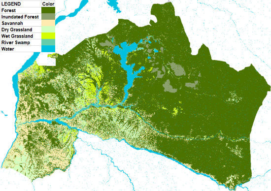
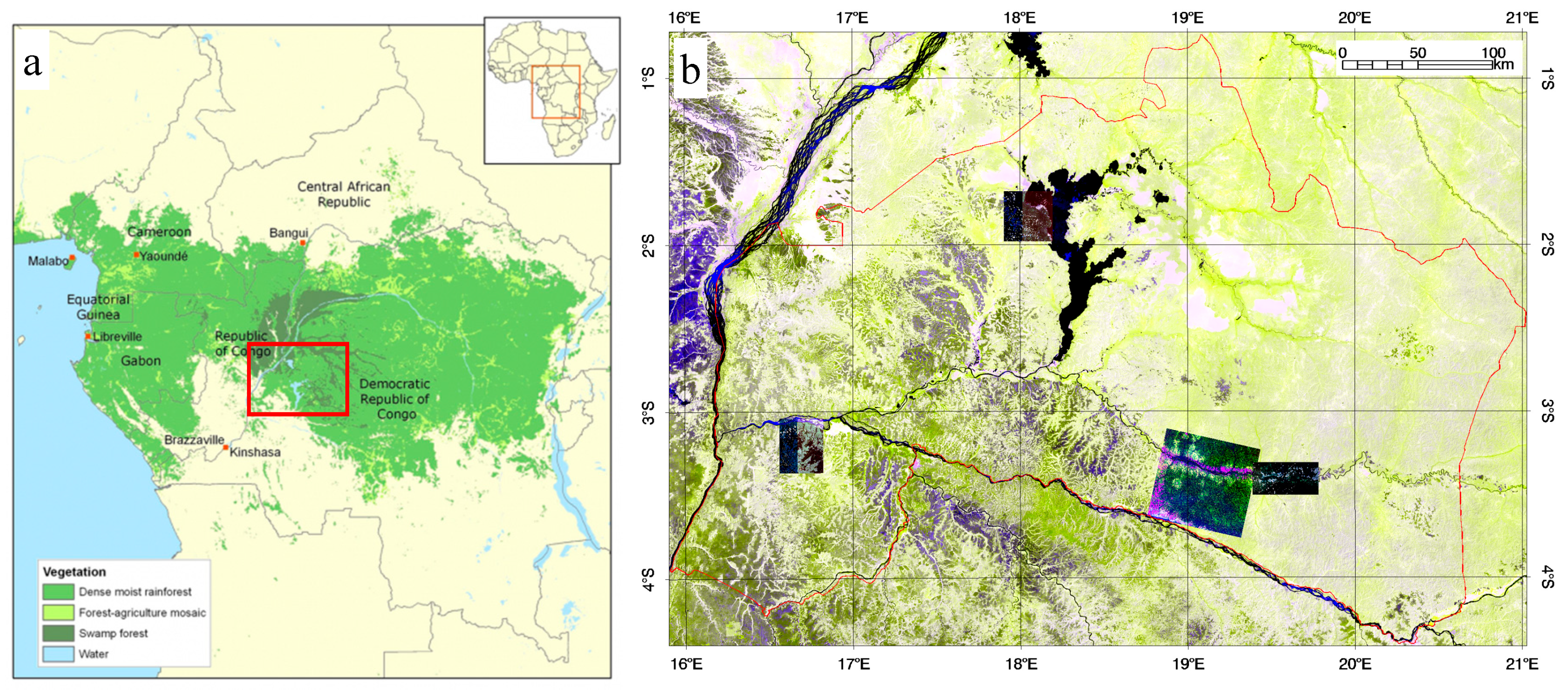
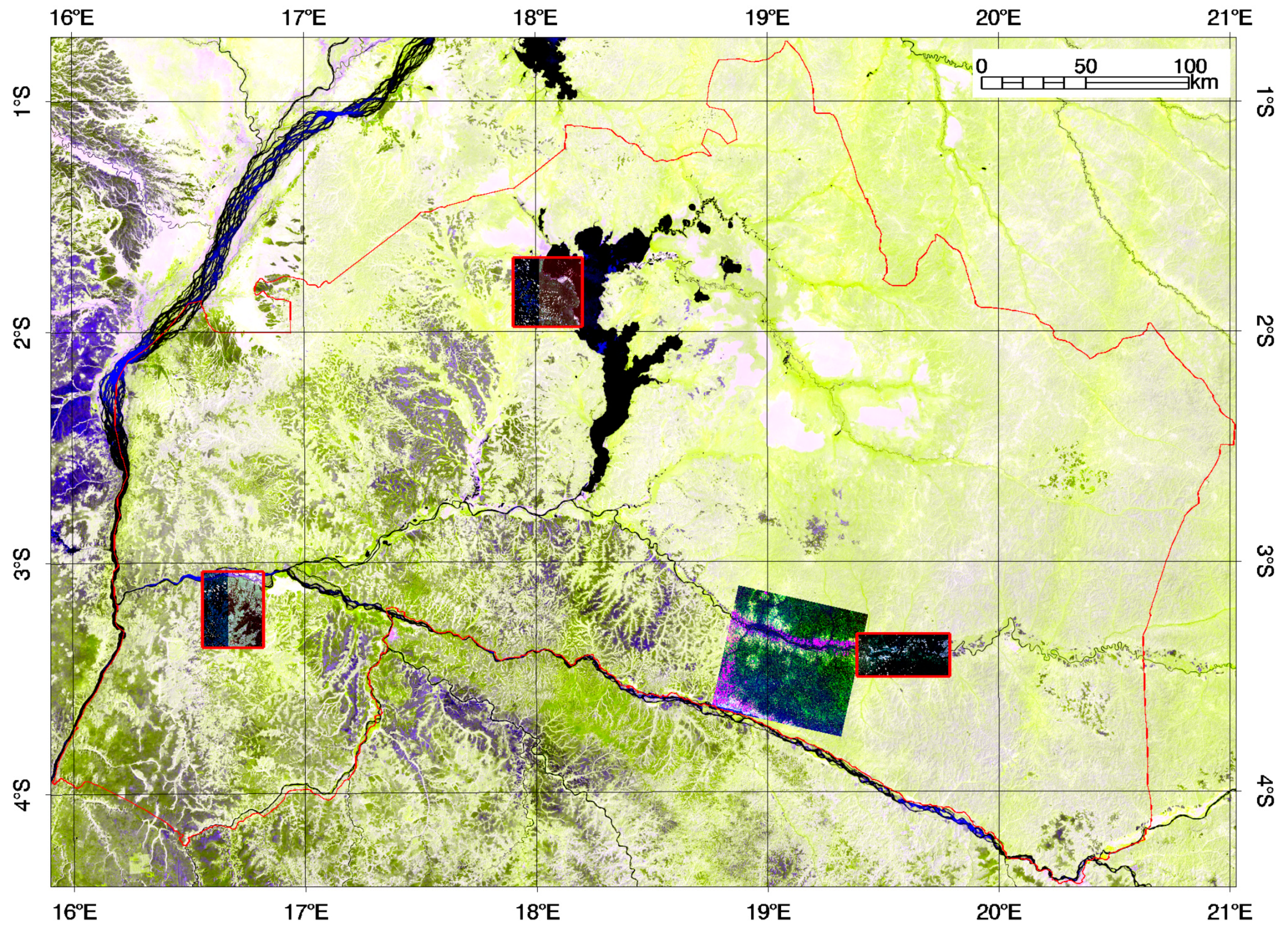
2.1. Region of Interest (ROI): Mai-Ndombe District in DRC
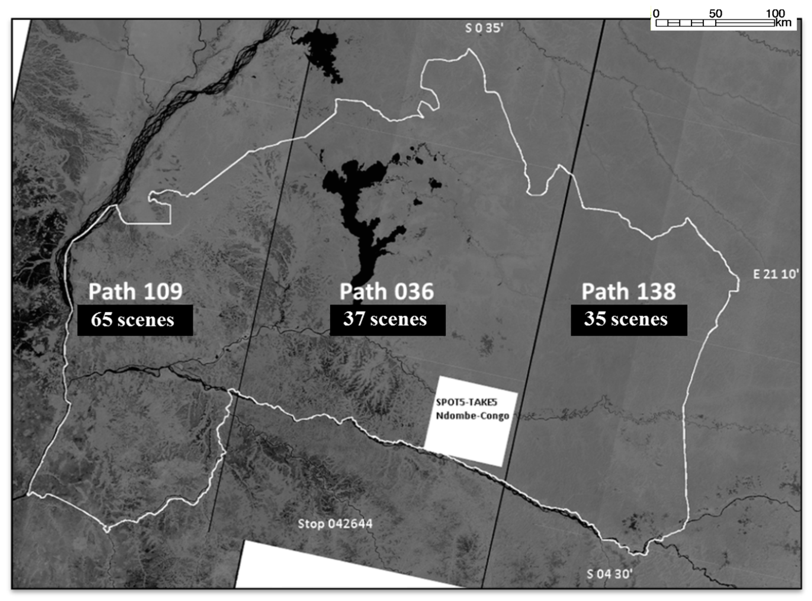
The Mai-Ndombe district is located in the Bandundu Province in the west of DRC, bordering the Congo River and the Republic of Congo. The area is very rich in biodiversity and endemic species (Bonobo). However, for many years this area has been facing high rates of deforestation and forest degradation caused by charcoal production for cities, especially due to the proximity of the capital Kinshasa, slash and burn agriculture, and industrial logging. The district covers an area of 128,789 km2 with its center geographical coordinates around [18°31′E; 2°42″S].
It is part of the humid tropics with primary and secondary forests, interspersed by swamp forest in humid lowlands and wet meadows, inundated forests in proximity of waterbodies, especially in the north, and savannahs predominantly in upland areas. There is a distinctive dry season from June to September, followed by the rainy season until December. The region has a north–south humidity gradient with the south being drier. Figure 1 shows the location of the Mai-Ndombe district and an overview of the very-high-resolution (VHR) data for validation.

2.2. Satellite Data

The study is based on C- and L-band space-borne SAR data. C-band SAR data is from the CSAR sensor on the operational satellites Sentinel-1A and 1B (S1A and S1B) [34] from the European Copernicus program. L-band SAR is from the Phased Array type L-band SAR (PALSAR-1 and -2) [35,36] on the Advanced Land Observing Satellites (ALOS-1 and -2) from the Japan Aerospace Exploration Agency (JAXA).

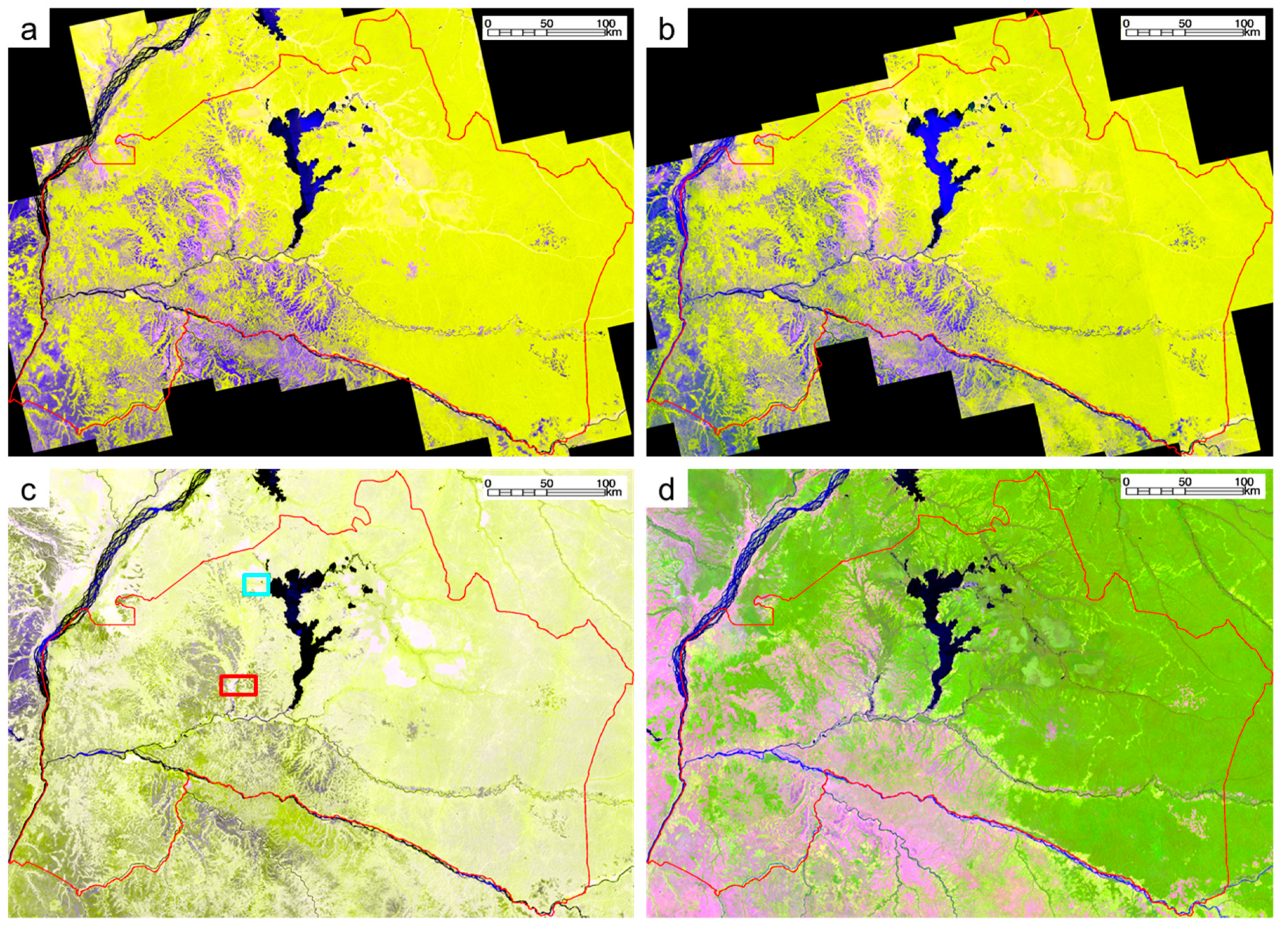
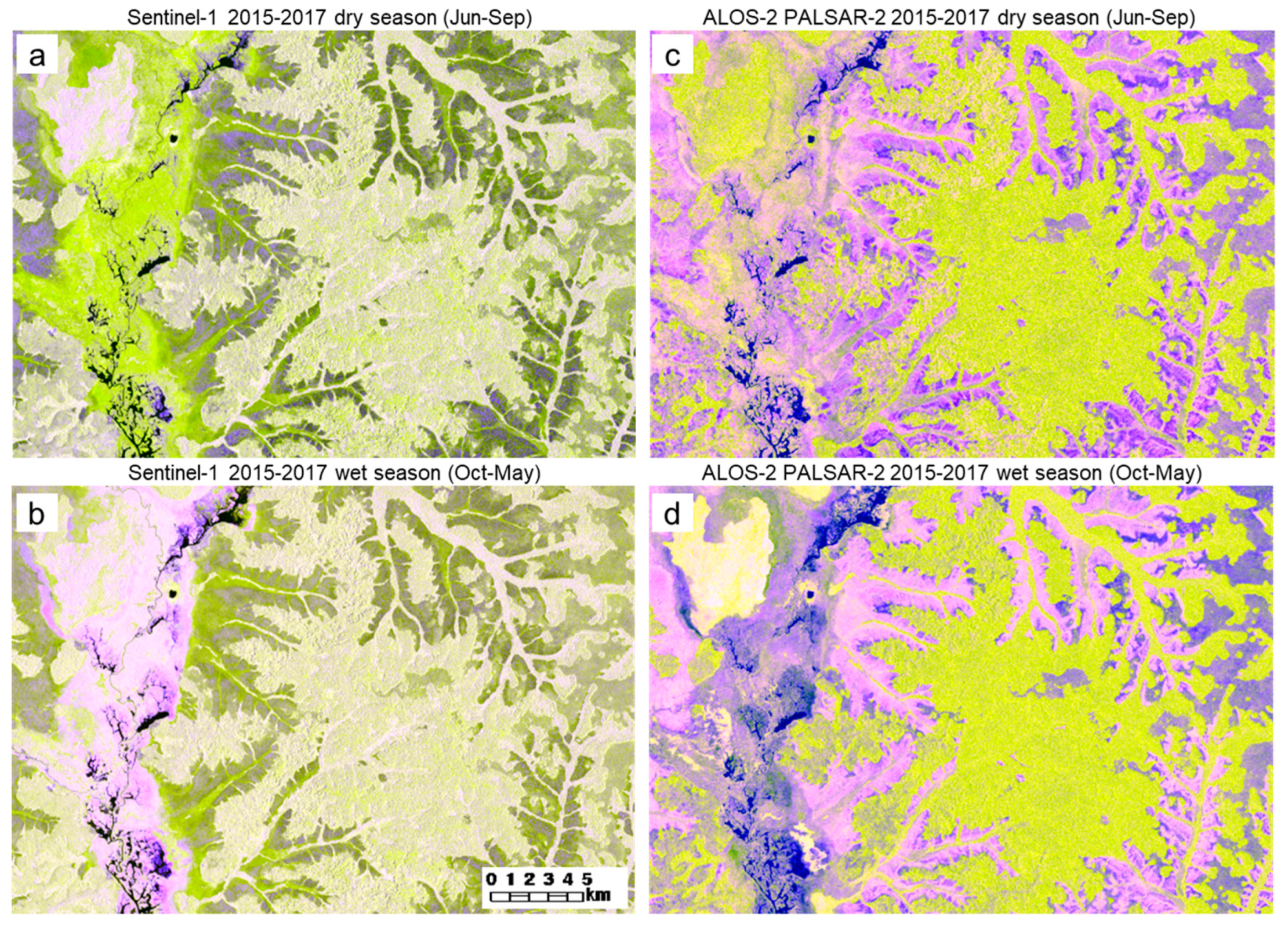
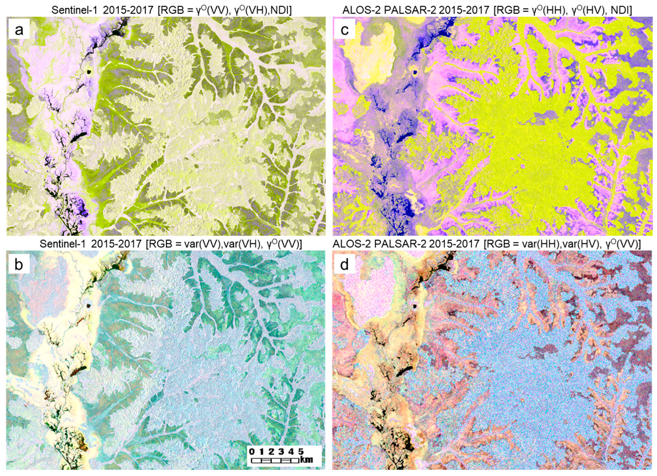
2.2.1. Sentinel-1 A and B CSAR (2015–2017)

The two identical S1A and S1B have been launched on 3 April 2014 and 25 April 2016, respectively, circumnavigating the whole earth on a 12 day repeat cycle. Data over the ROI are covered only by descending paths 109, 036, and 138 and acquired only by S1A on a 12 day revisiting cycle (Figure 2). Prior to October 2016, paths 036 and 138 were only acquired sporadically. The Sentinel-1 data set processed in this study covers the period April 2015–December 2017 with acquisitions in dual polarized interferometric wide swath mode (IW) processed at Ground Range Detected (GRD) level-1 freely available from the Copernicus Open Access Hub (https://scihub.copernicus.eu/). The dual polarization is in VV and VH, i.e. emitted in vertical (first V) and received (second V/H) in vertical and horizontal (H) polarization.

2.2.2. ALOS PALSAR (2007–2010) and ALOS-2 PALSAR-2 (2015–2017)

ALOS-2 PALSAR-2 [36] was launched on 24 May 2014 as a follow up mission of ALOS PALSAR [35] that was operational from 2006 to 2011.
The processed mode in this study acquired over the ROI is the fine beam dual (FBD) strip map mode in HH and HV polarization. PALSAR-2 data is used for direct comparison and combined used with Sentinel-1 data, whereas PALSAR is used in comparison as a historical reference as it turned out to be better calibrated than PALSAR-2. PALSAR-2 calibration has been updated on 28 March 2017 [37]. However, 2015 and 2016 data from ALOS-2 have been acquired prior to the update. JAXA’s correction values have been applied during the pre-processing stage but did not fully correct for the calibration error.
In all, 347 PALSAR and 196 PALSAR-2 FBD scenes have been acquired, covering each pixel 5–7 times and 3–6 times, respectively (Figure 3), not considering overlap between neighboring scenes. PALSAR data have been provided in level 1.1 by both ESA and JAXA, whereas PALSAR-2 level-1.1 data has been provided only by JAXA. Both PALSAR (/-2) acquisition plans gave priority to the dry season, but for each sensor at least one measurement per pixel has been acquired over the wet season. Although ALOS and ALOS-2 are commercial satellite programs, this project benefited from several research data grants (see Acknowledgements) and nearly all PALSAR (/-2) FBD acquisitions from ascending orbits were available in this study.

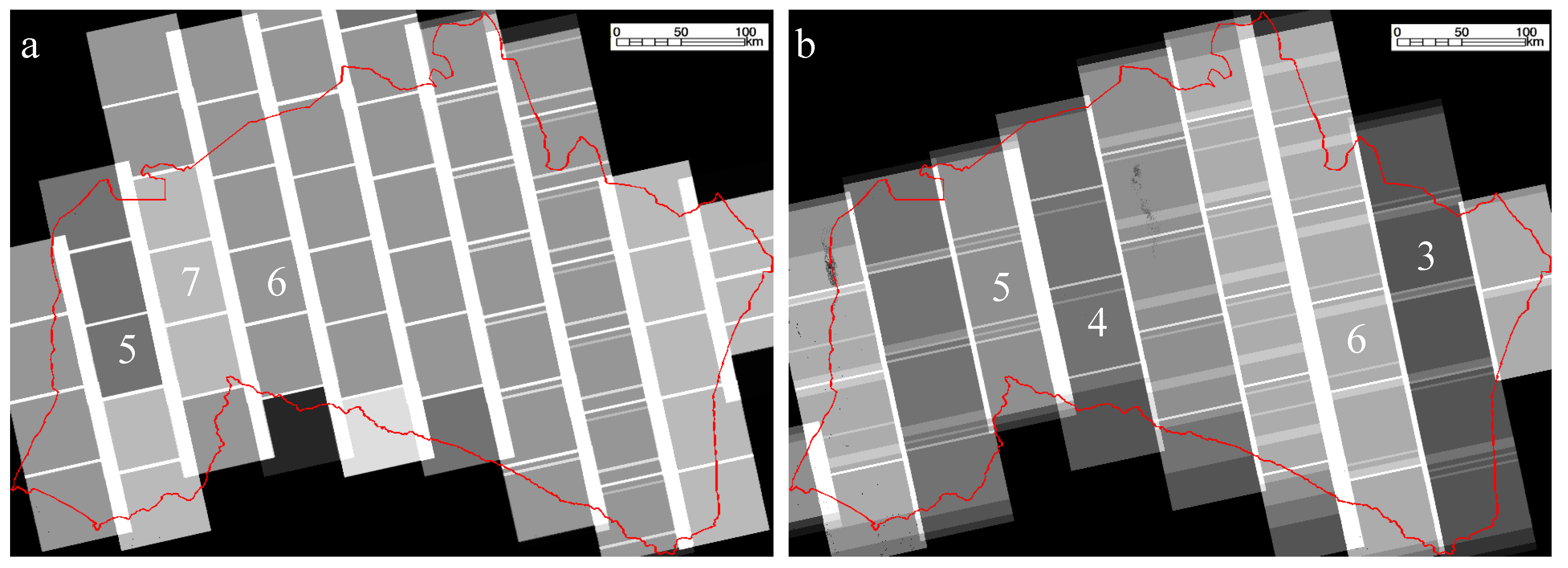
2.3. Pre-Processing and Mosaicking

Since the 1990s, Norut (now NORCE) has developed its in-house Generic SAR processing system, called GSAR [38], that has been used for pre-processing as well as to extract the statistical parameters for each pixel over a given data stack/time period.
All SAR data were first geocoded, radiometrically calibrated, terrain and slope corrected [39] on the same 30 m Universal Transverse Mercator (UTM) grid of zone 34S into gamma naught (γ°) backscatter for both, co- and cross-polarized bands (γ°[copol] and γ°[xpol]), i.e., VV and VH for Sentinel-1 and HH and HV for PALSAR and PALSAR-2. The 1 arc-second (~30 m resolution) digital surface model (DSM) from the Shuttle Radar Topography Mission (SRTM) [40,41] from the year 2000 was used for the pre-processing. Since the topography of the Mai-Ndombe district does not include high mountains and only a few steep slopes, the pixels affected by topographic-induced SAR shadow or overlay are negligible. Furthermore, ALOS-2 data from 2015 and 2016 have been corrected for JAXA’s initial error in radiometric calibration factors given in the data according to [37].
Following the pre-processing, all SAR data were statistically analyzed with the GSAR software suite establishing mean and variance images of γ° for each polarization band and each single-year and multi-year period in 2007–2010 for PALSAR and 2015–2017 for Sentinel-1 and PALSAR-2. Mean γ° images were also established for the wet and dry seasons using all October–May and June–September scenes, respectively. The normalized difference index (NDI) bands were calculated with the mean images by
N D I = γ ° [ copol ]     γ ° [ xpol ] γ ° [ copol ]   +   γ ° [ xpol ] .
Figure 4 illustrates the five image bands that are available as features in a multi-variate classification for each sensor and time period.
Mean dual-polarized mosaics are represented in red–green–blue channels as RGB = [γ°[copol]; γ°[xpol]; NDI]. Figure 5 shows the multi-year averaged mosaics for PALSAR (2007–2010), PALSAR-2 (2015–2017), and Sentinel-1 (2015–2017) along with an optical Landsat-8 mosaic as reference. Averages based on data from the wet season show significantly different backscatter signatures compared to averages based on the dry season in some areas, especially those with less vegetation. This has been shown to be the case even on a global scale on a 0.05 decimal degree grid by [27]. The cause of this is due to the differences in ground humidity, flooding, and vegetation foliage. Examples of such different signatures for both C- and L-band SAR are shown in Figure 6, which is a detailed view of the red rectangle in Figure 5. Although the dry season is in general very distinctive, the wetness and soil humidity of the rest of year is hard to quantify because of different acquisition times and specifically few acquisitions during the wet season from PALSAR and PALSAR-2. Furthermore, climate change makes the historically established seasonal periods less reliably defined. A different approach to use the seasonal variability is therefore to use the variance of each pixel of the whole time series instead of specific seasons. Figure 7 shows the yearly averaged mosaics and RGB composites representing the variance of co- and x-pol backscatters and γ°[co-pol]. These variables are used in different multi-variate combinations in a maximum-likelihood classification (MLC) [39] for forest land cover.

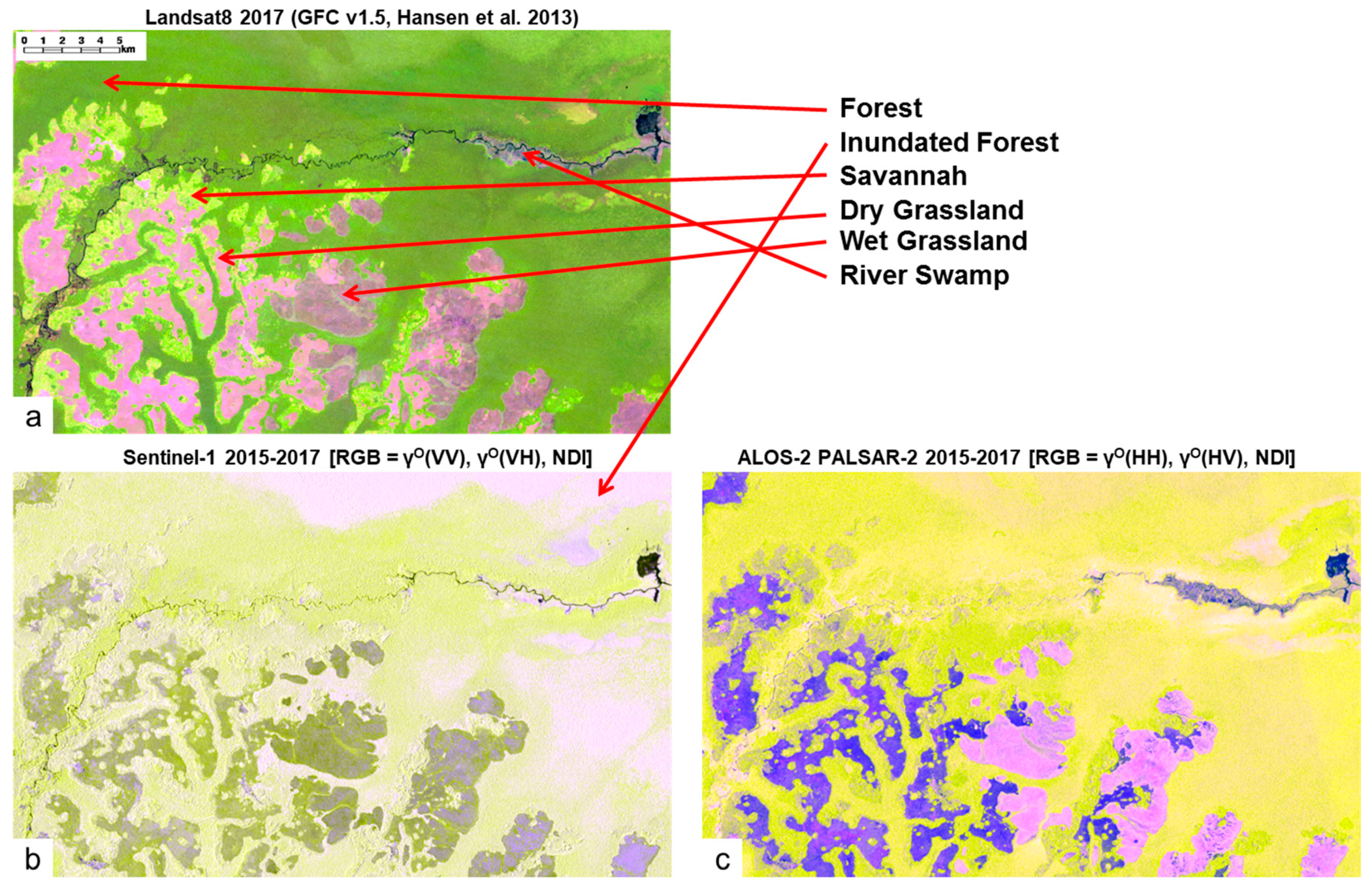
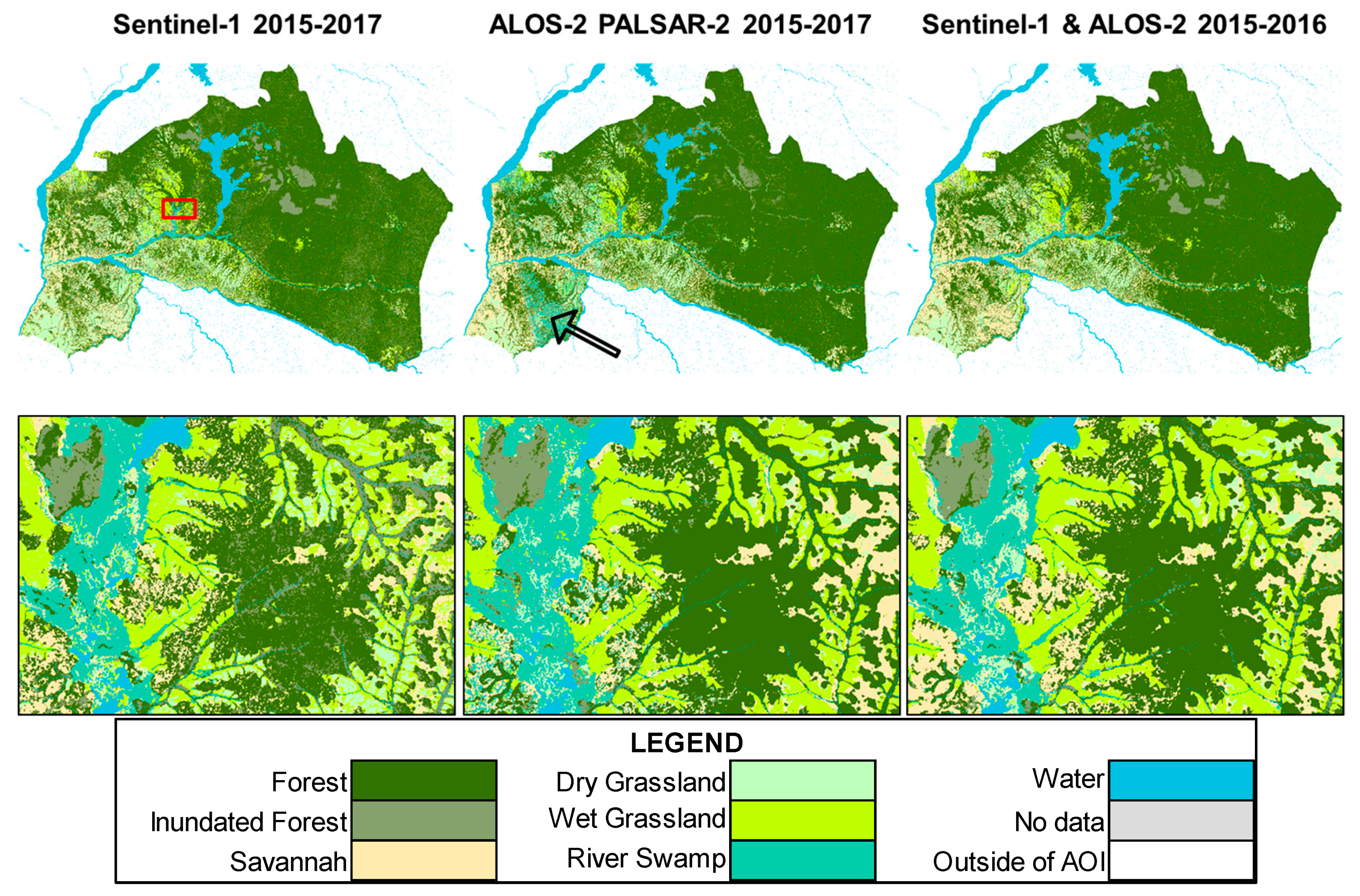
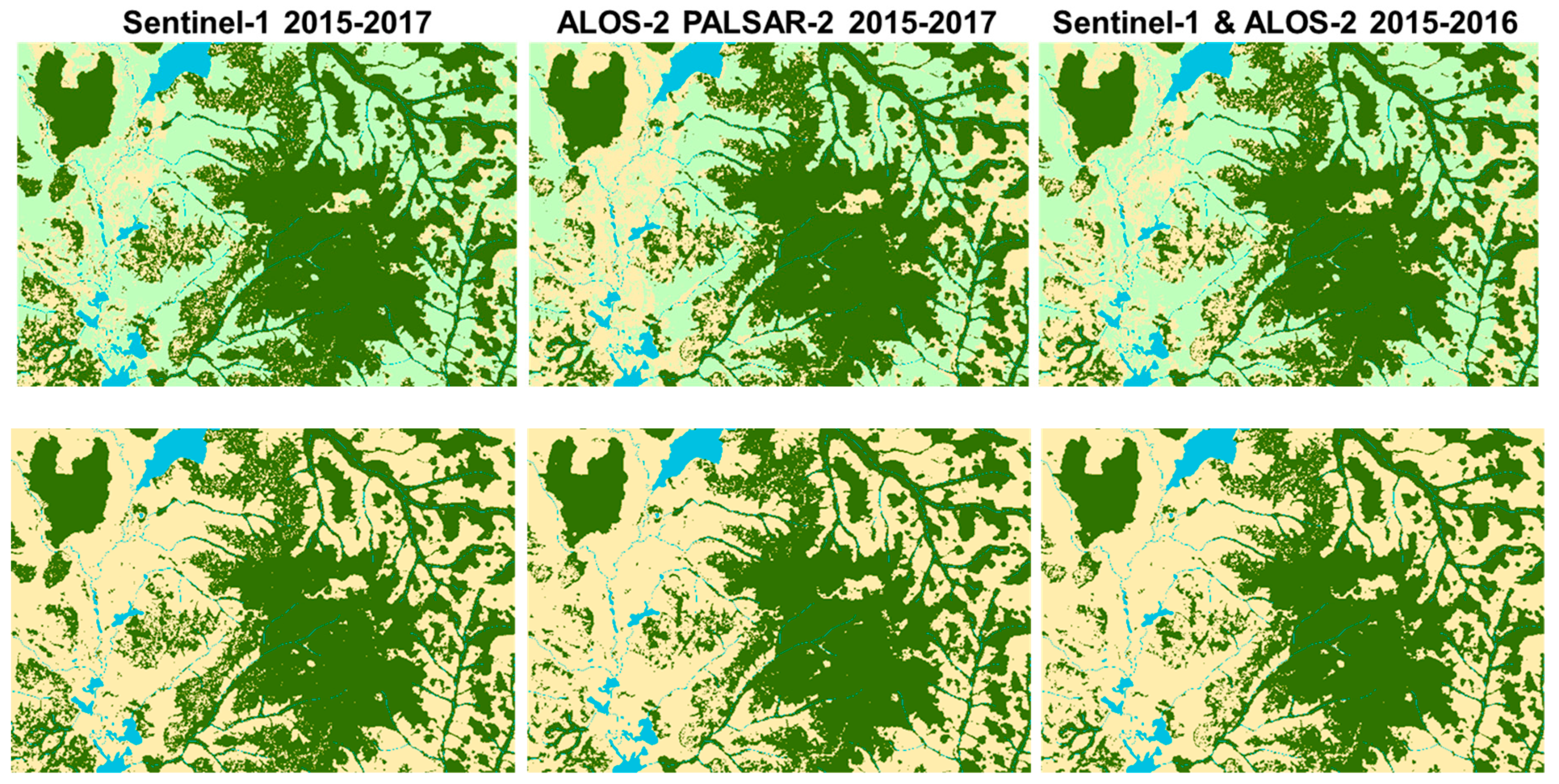
2.4. Maximum-Likelihood Classification into Forest and Land Covers (FLC)

During fieldwork in March 2013 northwest of Lake Mai-Ndombe [42], several areas that could be directly compared to SAR signatures were identified. Based on these observations and VHR optical data from GoogleEarth and RapidEye satellites, shapefile polygons of homogeneous training areas for six different land cover classes were assigned and used for a supervised MLC [43]. The six forest land cover (FLC) classes identified are forest, inundated forest, savannahs, predominantly dry grassland, predominantly wet grassland, and river swamps. Figure 8 shows examples of such areas that were recognized. A new water mask was constructed by using existing water mask shapefiles of lakes and rivers, the water mask extracted from the Facet Atlas [44], and by thresholding the cross-polarized SAR data.
The MLC has been chosen for classification because of several reasons; among those are: MLC is based on probability calculations assuming a Gaussian distribution of the signature for each class, which simplifies future operational implementation and allows for automatic use once the signatures are known for each class and variable; MLC is a general and widely distributed tool in most geographic information system (GIS) and image processing software and the results should therefore be easily reproducible; MLC [45] performed clearly better compared to all, but neural network classifier (NNC), supervised classification methods from the ENVI software (https://www.harrisgeospatial.com/Software-Technology/ENVI) suit that have been test run for this study. The NNC results were very similar to MLC results in accuracy. The calculated probabilities easily allow assigning super classes when the reference validation data does not include all six classes. All classification results have then been filtered with a 3 × 3 pixel majority window, so that less than five adjacent forest pixels, a minimum of 0.45 ha, would not be considered as forest according to the 0.5 ha forest area definition
The aim of the study is to investigate different combination of variables in a multi-variate MLC classification from single C-/L-band and multi-frequency, C-, and L-band combined. The different combinations of variables are based on:
  • The yearly averaged SAR backscatters, i.e., the three variables per sensor; mean(γ°[copol2017]), mean(γ°[xpol2017]), and NDI2017 for the year 2017.
  • The multi-year averaged SAR backscatters, i.e., the three variables per sensor mean(γ°[copol2015–2017]), mean(γ°[xpol2015–2017]), and NDI2015–2017 for the years 2015–2017.
  • The seasonally averaged backscatter for the dry and wet seasons, i.e., four variables per sensor; mean(γ°[copoldry]), mean(γ°[xpoldry]), mean(γ°[copolwet]), and mean(γ°[xpolwet]).
  • The statistical parameters mean and variance from the three-year period 2015–2017, four variables per sensor; mean(γ°[copol2015–2017]), mean(γ°[xpol2015–2017]), var(γ°[copol2015–2017]), and var(γ°[xpol2015–2017]).

2.5. Validation and Inter-Comparison Approach

The general approach to estimate the accuracy and quantifying uncertainty of land cover maps is done by comparing the produced maps with a reference sample data set via a confusion matrix [46]. The main purpose in our case is however to inter-compare the different combinations of variables in the MLC. As reference data set, three Pléiades images, two from 19 and one from 21 November 2016 (© Centre National D’Etudes Spatiales (CNES)/AirbusDS) in 50 cm resolution and a SPOT-5 scene (©CNES) dated 25 June 2015 in 5 m resolution from the SPOT5-Take5 program were made available through ESA and the Centre National D’Etudes Spatiales (CNES) (Figure 9). We follow the approach of [47] based on a systematic sampling grid. As we have trained the MLC with in situ knowledge, RapidEye imagery from 2013, and GoogleEarth, the SPOT5 and Pléiades VHR data are independent and solely used for validation. The Pléiades images cover an area of about 1000 km2 each and have been sampled on a regular 2.1 km grid for visual interpretation. The SPOT-5 scene covers an area of about 3600 km2 and has been sampled on a 4.2 km grid. The FLC maps include six land cover/vegetation classes. A reliable manual interpretation from optical satellite images did in general not allow a better differentiation than into forest, savannah, and grassland (FSG) as the other classes were not abundant in the VHR images and difficult to interpret visually. The samples where therefore interpreted manually into FSG samples considering the majority of each land cover in a square area of 0.5 ha, i.e., a 70 m × 70 m square, following the forest definition. In total, 924 samples were interpreted: 709 forest, 144 savannah, and 71 grassland samples.
Hence, we first reclassified the FLC land cover maps of the MLC into three-classes FSG maps; forest therefore includes the original “forest” and “inundated forest” class, grassland includes the dry and wet grassland classes and to reclassify “river swamp”, we choose the forest, savannah, or grassland class with the highest probability from the MLC. For the final forest/non-forest (FNF) validation, savannah and grassland are considered as non-forest. As a final step, all classification in 30 m resolution are filtered with a 3 × 3-pixel majority window.

3. Results

The MLC was applied on each SAR sensor dataset alone, PALSAR (2007–2010) as a historic reference, PALSAR-2, Sentinel-1, and on a combined PALSAR-2/Sentinel-1 data set (2015–2017) with the four combinations of variables described in Section 2.4. Figure 10 shows a comparison of the results from Sentinel-1, ALOS-2, and Sentinel-1/ALOS-2 combined using the multi-year statistical parameters, mean and variance, of the co- and cross-polarization backscatters γ°. As Table 1 shows, this feature combination gave in general the highest accuracies.
The left panel of Figure 10 shows that Sentinel-1 results can be quite noisy in the forested areas. The reason for this could be that C-band SAR penetrates only a little in the canopy and its signature therefore reflects also height differences in the upper canopy surface in inhomogeneous mixed forest that L-band will not see as it penetrated deeper in the canopy and will smooth out the canopy surface effects. C-band however seems to better distinguish lower biomass land covers, such as savannah, wet, and dry grassland up to a certain biomass level, above which C-band will saturate and classify as forest. Somewhat surprisingly, it seems that C-band also distinguishes inundated forest from forest better than L-band does. This could be due to this specific type of inundated forest, which might be a much lower biomass forest than the surrounding tropical forest. This still needs further investigation. The black arrow in the PALSAR-2 result indicates a vast misclassification area into river swamp in a particular satellite path which we anticipate is mainly due to the calibration factor error in 2015 and 2016 ALOS-2 data or do to the low ALOS-2 coverage during the wet seasons. The use of both sensors, ALOS-2 and Sentinel-1 (right panel in Figure 10), clearly seems to better distinguish the land cover areas, smoothing out the noise in forest areas of Sentinel-1 and still keeping a better distinction between savannah, wet, and dry grassland. Figure 11 shows the derived FSG and FNF results from the same MLC variable combination and enlarged area as in Figure 10.
The FSG and FNF results shown in Figure 11 and the corresponding results from all different applied variable combinations have been validated according to the approach described in Section 2.5. and are presented in Table 1. The different feature combinations using Sentinel-1 data have accuracies of 82% ± 3% with a kappa of 0.48% ± 0.07% and 87% ± 4% (kappa of 0.61 ± 0.1) for FSG and FNF, respectively. For the L-band SAR data, both from ALOS and ALOS-2, FSG accuracies are around 90% ± 1% (kappa 0.68 ± 0.03) and FNF accuracies are around 92% ± 1% (kappa 0.75 ± 0.02). For Sentinel-1 data, where we have continuous time series on a 12-day cycle, the use of temporal variability, either by dividing into a wet and dry data set or by using the variance over the whole data set improves the FSG and FNF classification results significantly by about 5–6 percent points and increasing kappa from 0.42 to 0.55 and from 0.52 to 0.70, respectively. For L-band SAR, which is in general clearly better suited for forest and land cover classification, using the variability improves the results only by 1–2 percent points for ALOS. For ALOS-2, there is no improvement, i.e., an insignificant decrease and increase in accuracy and kappa, respectively. We assume that the main reason that there has been no improvement by using multi-year data including differentiating wet and dry seasons and statistics compared to only 2017 data is due to (1) the radiometric correction issue for 2015 and 2016 data and (2) that, also valid for ALOS, ALOS-2 acquisitions have a strong acquisition focus on the dry season, and much less acquisitions per pixel in general which could be the main reason for the quite stable results. This will be further discussed in Section 4.
Table 2 and Table 3 show the confusion matrixes for the FSG and FNF classification using the Sentinel-1 and ALOS-2 co- and cross polarized 2015–2017 average backscatters and their variances (last line in Table 1). They indicate that there is a tendency to classify into higher biomasses, i.e., grassland toward savannah and savannah toward forest) and the producer accuracy increases with higher biomass classes. However, there seems to be no strong bias in the user accuracies. Note that majority filtering took place after classifying FNF from FSG, and Table 3 is therefore not directly derived from Table 2.

4. Discussion

4.1. Inter-Comparison between Single and Multi-Frequency SAR Results

In agreement with earlier studies, it is no surprise that the results reflect that L-band SAR is in general better suited for forest mapping than C-band SAR as C-band SAR saturates at much lower biomass vegetation than L-band. The results however show that the use of statistics of the better temporal resolution of C-band Sentinel-1 time series acquisition compared to less frequent L-band PALSAR can make up for about half of the difference in accuracies.
The general impression for all SAR sensors is that temporal filtering to reduce speckle and single acquisition conditions improves classification results. As long as we can also neglect inter-annual forest change compared to the mapping errors for example when building a baseline forest map, integration over a multi-year time period for data sets with very few yearly acquisitions, like PALSAR-1 and -2, also improves the results. This is especially the case if the temporal resolution of the data series does not even resolve the seasonality between dry and wet periods. Dividing a data stack into specific seasonal averaged products or extracting the statistics, even if that requires a multi-year period, clearly increases the accuracy and kappa value. This shows clearly in the PALSAR-1 and Sentinel-1 results, with improved accuracies of 1–2 percent points and 4–5 percent point, and improved kappa values by about 0.05 and 0.1, respectively. We assume that the reason why this does not show in the PALSAR-2 results is partly because of the calibration issue of 2015 and 2016 PALSAR-2 level 1.1 products, as well as the fact that PALSAR-2 acquisitions are too few (3–6 acquisitions per pixel) to define significant statistical values. Unfortunately, our available PALSAR-2 acquisitions in 2017 did not allow for a division into wet and dry mosaics over the whole area. All four PALSAR-2 feature combinations show therefore very similar results.
The temporal resolution of Sentinel-1 acquisitions of 12 days, i.e., 30 acquisitions per year, would probably allow integrating the data set also over a single year instead of a multi-year period to clearly detect seasonal differences and extract significant statistical values. For comparability with the L-band data set however, this has not been studied in detail, but the slightly better results of the 2017 averaged mosaics versus the 2015–2017 averaged mosaics clearly support this assumption.
In general, our approach to either use seasonal averages or statistics (mean and variance) is very similar as we assume that the main variance of SAR signatures is due to differences in humidity and foliage, especially in low vegetated areas, and results therefore should be and are very similar. Although, it seems that using the yearly statistical values, mean backscatter and variance, gives slightly better results. As the locals of the region reported to us during the field campaign that the rainy and dry season patterns have changed in their occurrence during the year, probably due to climate change, our definition of wet and dry seasons, based on historic weather observations might not correctly apply and even less in the future. The variability between wet and dry conditions might therefore be better reflected with statistical parameters instead, or each observation would need to be confirmed individually by meteorological observation.
In this study, we have only taken temporal statistics into account and not textural statistics in space which would have reduced our spatial resolution. The temporal resolution of Sentinel-1 could even allow to consider other statistical parameters, for example different percentiles and the temporal distribution of SAR signatures. Such dense time series are of course also better suited to clearly detect and confirm changes with time series analysis tools such as the Bfast algorithm [19,48]. A more specific study of the backscatter time series and seasonality could also be of particular interest in regard to forest ecology or physiology but is beyond the scope of this paper.
The highest accuracies are obtained when combining C- and L-band in a multi-frequency approach. Nevertheless, the results show that C-band does not seem to improve the L-band results when only using yearly or multi-year mosaics without using the seasonality or statistics. When C-and L-band are combined, it is clear that the Sentinel-1’s strength lies in the dense time series, and that their temporal statistics and the multi-seasonal division are the main reasons of the improvements in accuracies compared to L-band ALOS-2 alone. Both the FSG and the FNF maps improve by about one percent point combining C- and L-band SAR compared to L-band alone.

4.2. Comparision with Global Forest Maps

A main reference data set for forest and forest change maps is the GFC program [6] based on the Landsat archive. It is also the data set that is widely used to establish baseline forest reference maps for the carbon emission reporting in REDD+ programs. JAXA provides yearly forest maps based on ALOS and ALOS-2 [31,32]. Both data sets have been validated with the same VHR data set and compared to our SAR results (Table 4). According to the final DRC Emission Reductions Program Document from 2016 [49], the forest definition has been set to a minimum crown cover of 30%, minimum land area 0.5 ha, and minimum tree height of 3 m. However, in the Emission Reductions Program Idea Note (ERPIN) [50] and based on [6], forest (primary and secondary) is defined with a crown cover higher than 50% and woodland, defined as crown cover of 26%–50%, is defined as non-forest. Our validation shows clearly that a crown cover higher than 50% corresponds better to a forest definition than a minimum crown cover of 30% in GFC data. Table 4 summarizes the accuracy assessment of these two global forest maps compared to our SAR-based results. Shimada [51] reported global accuracies for ALOS-2 forest maps of 88.21% and 87.77% for the years 2015 and 2016, respectively, which are in good agreement with our validation results.

5. Conclusions

This study compared forest land cover maps from single (C- and L-band) and multi-frequency satellite SAR data applying different feature combination in a supervised MLC. The SAR results and global forest maps from GFC and JAXA were then validated with the same sampled and visually interpreted VHR optical satellite data and compared. The accuracy assessment shows that C-, L-, and C/L-band combined all achieved FNF map accuracies above 90% and higher accuracies than global forest maps from both Landsat [6] and ALOS-2 [32]. A few yearly observations with L-band SAR still give higher accuracies than dense time series of C-band Sentinel-1, but it is clear that the dense time series and the operational acquisition plan of Sentinel-1 provides an enormous improvement, showing that Sentinel-1 can be used complementarily and interoperable to optical data for forest mapping. Forest–savannah–grassland and FNF classification with L-band SAR are about 6 percent points and 2 percent point more accurate than with C-band, respectively. However, the combination of C- and L-band combined shows that C-band can improve L-band results to obtain accuracies of 90.04% (kappa of 0.72) and 93.29% (kappa of 0.80) for FSG and FNF classifications, respectively. The results also indicate that using temporal statistics, at least mean and variance, considerably improves the accuracies. They can be used instead of a seasonal separation of data stacks, especially if the seasons are either not clearly defined, have strong inter-annual variations, are not known, or might have shifted because of climate change. Without any doubt, dense data stacks of L-band, representing all seasons with clear statistics will further increase the potential of SAR classification of forest land cover and even for sub-classes dividing into different vegetation types. The ESA L-band SAR candidate mission ROSE-L [52] should therefore be of high interest for the land cover science community, especially in the tropics and high latitudes with persistent cloud cover.

Author Contributions

J.H. conceived, designed, and led the project, as well as processed and analyzed the data; H.H. contributed with software tools development and scripting the software tools into processing lines, as well as proofreading the paper.

Funding

This research was funded by the European Space Agency DUE Innovator III project “SAR for REDD”, contract no. 4000116151/15/I-NB.

Acknowledgments

Satellite data have been provided through a GSC-DA grant from ESA and JAXA during EU FP7 Project ReCover, ESA cat-1 proposal no. 27689, JAXA ALOS-2 RA4 proposal 1205, and the Copernicus Open Access Hub. This paper and figures contain modified Copernicus Sentinel-1 data 2015–2017, ALOS PALSAR [original data © Japan Aerospace Exploration Agency (JAXA) 2007–2010], ALOS-2 PALSAR-2 [original data © Japan Aerospace Exploration Agency (JAXA) 20015–2017], and Landsat-8 data [original data © NASA/U.S. Geological Service (USGS), processed by GFC v1.5]. SPOT-5 data were provided by CNES and ESA under the Spot5-Take5 project and the SPOT Pleiades satellite data by CNES (2015,2016) and distributed by Airbus DS (2015/2016). We wish to thank OSFAC staff, especially the Director L. Mane, A. Mazinga and C. Singa, all participants during fieldwork in the Mai-Ndombe district 2013 and 2016, and our NORCE colleagues, Y. Larsen and T. Grydeland for continuously maintaining and improving the SAR processing software.

Conflicts of Interest

The authors declare no conflict of interest.

References

  1. Van der Werf, G.R.; Morton, D.C.; DeFries, R.S.; Olivier, J.G.J.; Kasibhatla, P.S.; Jackson, R.B.; Collatz, G.J.; Randerson, J.T. CO2 emissions from forest loss. Nat. Geosci. 2009, 2, 737–738. [Google Scholar] [CrossRef]
  2. Gullison, R.E.; Frumhoff, P.C.; Canadell, J.G.; Field, C.B.; Nepstad, D.C.; Hayhoe, K.; Avissar, R.; Curran, L.M.; Friedlingstein, P.; Jones, C.D.; et al. Tropical Forests and Climate Policy. Science 2007, 316, 985–986. [Google Scholar] [CrossRef] [PubMed]
  3. The United Nations Framework Convention on Climate Change (UNFCCC). 2015 Paris Agreement English. Available online: https://unfccc.int/files/meetings/paris_nov_2015/application/pdf/paris_agreement_english_.pdf (accessed on 27 September 2019).
  4. Sukhdevb, P.; Prabhua, R.; Kumara, P.; Bassic, A.; Patwa-Shaha, W.; Entersa, T.; Labbatea, G.; Greenwalta, J. REDD+ and a Green Economy: Opportunities for a Mutually Supportive Relationship, UN-REDD Programme Policy Brief 2012, Issue #01. Available online: https://theredddesk.org/sites/default/files/resources/pdf/2012/unep_policy_brief.pdf (accessed on 27 September 2019).
  5. Herold, M.; Skutsch, M. Measurement, Reporting and Verification for REDD+: Objectives, Capacities and Institutions. In Realising REDD+: National Strategy and Policy Options; Angelsen, A., Brockhaus, M., Kanninen, M., Sills, E., Sunderlin, W.D., Wertz-Kanounnikoff, S., Eds.; Center for International Forestry Research (CIFOR): Bogor, Indonesia, 2009; pp. 85–100. ISBN 978-6-02-869303-5. [Google Scholar]
  6. Hansen, M.C.; Potapov, P.V.; Moore, R.; Hancher, M.; Turubanova, S.A.; Tyukavina, A.; Thau, D.; Stehman, S.V.; Goetz, S.J.; Loveland, T.R.; et al. High-Resolution Global Maps of 21st-Century Forest Cover Change. Science 2013, 342, 850–853. [Google Scholar] [CrossRef] [PubMed] [Green Version]
  7. Shimabukuro, Y.E.; Santos, J.R.; Formaggion, A.R.; Duarte, V.; Rudorff, B.F.T. The Brazilian Amazon monitoring program: PRODES and DETER projects. Glob. For. Monit. Earth Obs. 2012. [Google Scholar] [CrossRef]
  8. Instituto Nacional de Pesquisas Espaciais (INPE). Degrad. Available online: http://www.obt.inpe.br/OBT/assuntos/programas/amazonia/degrad (accessed on 27 September 2019).
  9. Instituto Nacional de Pesquisas Espaciais (INPE). Deter. Available online: http://www.obt.inpe.br/OBT/assuntos/programas/amazonia/deter (accessed on 27 September 2019).
  10. Global Forest Observations Initiative (GFOI). Available online: http://www.fao.org/gfoi (accessed on 27 September 2019).
  11. Carter, S.; Herold, M. Activities and Research Priorities of the GFOI R&D Coordination Component 2019; Global Forest Observations Initiative (GFOI): Rome, Italy, 11 February 2019; Available online: http://www.gofcgold.wur.nl/documents/GFOI/GFOI_RD_Priorities_2019.pdf (accessed on 11 December 2019).
  12. Global Forest Observations Initiative (GFOI). Integration of Remote-Sensing and Ground-Based Observations for Estimation of Emissions and Removals of Greenhouse Gases in Forests: Methods and Guidance from the Global Forest Observations Initiative, Edition 2.0; Food and Agriculture Organization: Rome, Italy, 2016; Available online: https://www.fs.fed.us/nrs/pubs/jrnl/2016/nrs_2016_penman_001.pdf (accessed on 11 December 2019).
  13. Reiche, J.; Lucas, R.; Mitchell, A.L.; Verbesselt, J.; Hoekman, D.H.; Haarpaintner, J.; Kellndorfer, J.M.; Rosenqvist, A.; Lehmann, E.A.; Woodcock, C.E.; et al. Combining satellite data for better tropical forest monitoring. Nat. Clim. Chang. 2016, 6, 120–122. [Google Scholar] [CrossRef]
  14. Hoekman, D.H.; Vissers, M.A.M.; Wielaard, N. PALSAR Wide-Area Mapping of Borneo: Methodology and Map Validation. IEEE J. Sel. Top. Appl. Earth Obs. Remote Sens. 2010, 3, 605–617. [Google Scholar] [CrossRef]
  15. Almeida-Filho, R.; Shimabukuro, Y.E.; Rosenqvist, A.; Sánchez, G.A. Using dual-polarized ALOS PALSAR data for detecting new fronts of deforestation in the Brazilian Amazônia. Int. J. Remote Sens. 2009, 30, 3735–3743. [Google Scholar] [CrossRef]
  16. Haarpaintner, J.; Almeida-Filho, R.; Shimabukuro, Y.E.; Malnes, E.; Lauknes, I. Comparison of ENVISAT ASAR deforestation monitoring in Amazônia with Landsat-TM and ALOS PALSAR images. In Proceedings of the Anais XIV Simpósio Brasileiro de Sensoriamento Remoto, Natal, Brasil, 25–30 April 2009; INPE: Brasilia, Brasil, 2009; pp. 5857–5864. [Google Scholar]
  17. Mermoz, S.; Le Toan, T. Forest Disturbances and Regrowth Assessment Using ALOS PALSAR Data from 2007 to 2010 in Vietnam, Cambodia and Lao PDR. Remote Sens. 2016, 8, 217. [Google Scholar] [CrossRef] [Green Version]
  18. Mermoz, S.; Réjou-Méchain, M.; Villard, L.; Le Toan, T.; Rossi, V.; Gourlet-Fleury, S. Decrease of L-band SAR backscatter with biomass of dense forests. Remote Sens. Environ. 2015, 159, 307–317. [Google Scholar] [CrossRef]
  19. Reiche, J.; Verhoeven, R.; Verbesselt, J.; Hamunyela, E.; Wielaard, N.; Herold, M. Characterizing Tropical Forest Cover Loss Using Dense Sentinel-1 Data and Active Fire Alerts. Remote Sens. 2018, 10, 777. [Google Scholar] [CrossRef] [Green Version]
  20. Reiche, J.; Hamunyela, E.; Verbesselt, J.; Hoekman, D.; Herold, M. Improving near-real time deforestation monitoring in tropical dry forests by combining dense Sentinel-1 time series with Landsat and ALOS-2 PALSAR-2. Remote Sens. Environ. 2018, 204, 147–161. [Google Scholar] [CrossRef]
  21. Bouvet, A.; Mermoz, S.; Le Toan, T.; Villard, L.; Mathieu, R.; Naidoo, L.; Asner, G.P. An above-ground biomass map of African savannahs and woodlands at 25 m resolution derived from ALOS PALSAR. Remote Sens. Environ. 2018, 206, 156–173. [Google Scholar] [CrossRef]
  22. Abdikan, S.; Sanli, F.B.; Ustuner, M.; Calò, F. Land Cover Mapping Using Sentinel-1 SAR Data. Int. Arch. Photogramm. Remote Sens. Spat. Inf. Sci. 2016, 61, 757–761. [Google Scholar] [CrossRef]
  23. Joshi, N.; Baumann, M.; Ehammer, A.; Fensholt, R.; Grogan, K.; Hostert, P.; Jepsen, M.R.; Kuemmerle, T.; Meyfroidt, P.; Mitchard, E.T.A.; et al. A Review of the Application of Optical and Radar Remote Sensing Data Fusion to Land Use Mapping and Monitoring. Remote Sens. 2016, 8, 70. [Google Scholar] [CrossRef] [Green Version]
  24. Mitchard, E.T.A.; Saatchi, S.S.; Woodhouse, I.H.; Nangendo, G.; Ribeiro, N.S.; Williams, M.; Ryan, C.M.; Lewis, S.L.; Feldpausch, T.R.; Meir, P. Using satellite radar backscatter to predict above-ground woody biomass: A consistent relationship across four different African landscapes. Geophys. Res. Lett. 2009, 36, L23401. [Google Scholar] [CrossRef]
  25. Santi, E.; Paloscia, S.; Pettinato, S.; Fontanelli, G.; Mura, M.; Zolli, C.; Maselli, F.; Chiesi, M.; Bottai, L.; Chirici, G. The potential of multifrequency SAR images for estimating forest biomass in Mediterranean areas. Remote Sens. Environ. 2017, 200, 63–73. [Google Scholar] [CrossRef]
  26. Wang, Y.; Hess, L.H.; Filoso, S.; Melack, J.M. Understanding the radar backscattering from flooded and nonflooded Amazonian forests: Results from canopy backscatter modeling. Remote Sens. Environ. 1995, 54, 324–332. [Google Scholar] [CrossRef]
  27. Koyama, C.N.; Watanabe, M.; Hayashi, M.; Ogawa, T.; Shimada, M. Mapping the spatial-temporal variability of tropical forests by ALOS-2 L-band SAR big data analysis. Remote Sens. Environ. 2019, 233, 111372. [Google Scholar] [CrossRef]
  28. Saatchi, S.; Marlier, M.; Chazdon, R.L.; Clark, D.B.; Russell, A.E. Impact of spatial variability of tropical forest structure on radar estimation of aboveground biomass. Remote Sens. Environ. 2011, 115, 2836–2849. [Google Scholar] [CrossRef]
  29. Le Toan, T.; Quegan, S.; Davidson, M.; Balzter, H.; Paillou, P.; Papathanassiou, K.; Plummer, S.; Saatchi, S.; Shugart, H.; Ulander, L. The BIOMASS mission: Mapping global forest biomass to better understand the terrestrial carbon cycle. Remote Sens. Environ. 2011, 115, 2850–2860. [Google Scholar] [CrossRef] [Green Version]
  30. Torres, R.; Snoeij, P.; Geudtner, D.; Bibby, D.; Davidson, M.; Attema, E.; Potin, P.; Rommen, B.; Floury, N.; Brown, M.; et al. GMES Sentinel-1 mission. Remote Sens. Environ. 2012, 120, 9–24. [Google Scholar] [CrossRef]
  31. The Japan Aerospace Exploration Agency (JAXA). Global PALSAR-2/PALSAR/JERS-1 Mosaic and Forest/Non-Forest Map. Available online: https://www.eorc.jaxa.jp/ALOS/en/palsar_fnf/fnf_index.htm (accessed on 27 September 2019).
  32. Shimada, M.; Itoh, T.; Motooka, T.; Watanabe, M.; Tomohiro, S.; Thapa, R.; Lucas, R. New Global Forest/Non-forest Maps from ALOS PALSAR Data (2007–2010). Remote Sens. Environ. 2014, 155, 13–31. [Google Scholar] [CrossRef]
  33. Ninth Consolidated Annual Progress Report of the UN-REDD Programme Fund. Available online: https://www.unredd.net/documents/programme-progress-reports-785/2017-programme-progress-reports/16758-ninth-consolidated-annual-progress-report-of-the-un-redd-programme-fund.html (accessed on 27 September 2019).
  34. European Space Agency (ESA). Sentinel-1: ESA’s Radar Observatory Mission for GMES Operational Services. ESA Communications, 2012. ESA SP-1322/1, ESTEC. Available online: https://sentinel.esa.int/web/sentinel/missions/sentinel-1 (accessed on 27 September 2019).
  35. The Japan Aerospace Exploration Agency (JAXA). About ALOS–PALSAR. Available online: http://www.eorc.jaxa.jp/ALOS/en/about/palsar.htm (accessed on 27 September 2019).
  36. The Japan Aerospace Exploration Agency (JAXA). ALOS-2 Project/PALSAR-2. Available online: https://www.eorc.jaxa.jp/ALOS-2/en/about/palsar2.htm (accessed on 27 September 2019).
  37. JAXA EORC/ALOS-2 Project Team. Update of the Radiometric and Polarimetric Calibration for the PALSAR-2 Standard Product. Available online: https://www.eorc.jaxa.jp/ALOS-2/en/calval/PALSAR2_CalVal_Result_JAXA_20170323_En.pdf (accessed on 27 September 2019).
  38. Larsen, Y.; Engen, G.; Lauknes, T.R.; Malnes, E.; Høgda, K.A. A generic differential InSAR processing system, with applications to land subsidence and SWE retrieval. In Proceedings of the ESA FRINGE Workshop 2005, ESA ESRIN, Frascati, Italy, 28 November–2 December 2005. [Google Scholar]
  39. Ulander, L. Radiometric slope correction of synthetic aperture radar images. IEEE Trans. Geosci. Remote Sens. 1996, 34, 1115–1122. [Google Scholar] [CrossRef]
  40. US Geological Service. USGS EarthExplorer. Available online: https://earthexplorer.usgs.gov/ (accessed on 27 September 2019).
  41. Farr, T.G.; Rosen, P.A.; Caro, E.; Crippen, R.; Duren, R.; Hensley, S.; Kobrick, M.; Paller, M.; Rodriguez, E.; Roth, L.; et al. The shuttle radar topography mission. Rev. Geophys. 2007, 45, RG2004. [Google Scholar] [CrossRef] [Green Version]
  42. Haarpaintner, J.D.; de la Fuente Blanco, F.; Enßle, P.; Datta, A.; Mazinga, C.; Singa, L.M. Tropical Forest Remote Sensing Services for the Democratic Republic of Congo inside the EU FP7 ‘ReCover’ Project (Final Results 2000-2012). Int. Arch. Photogramm. Remote Sens. Spat. Inf. Sci. 2015, 60, 397–402. [Google Scholar] [CrossRef] [Green Version]
  43. Richards, J.A. Remote Sensing Digital Image Analysis: An Introduction; Springer: Berlin, Germany, 1999; p. 240. [Google Scholar] [CrossRef]
  44. Mane, L.; Potapov, P.; Turubanova, S. Monitoring the forests of Central Africa using remotely sensed data sets (FACET), 2010. Forest Cover and Forest Cover Loss in the Democratic Republic of Congo from 2000 to 2010; South Dakota State University: Brookings, SD, USA, 2010; ISBN 978-0-9797182-5-0. [Google Scholar]
  45. L3 Haaris Geospacial Solutions. Maximum Likelihood. Available online: https://www.harrisgeospatial.com/docs/MaximumLikelihood.html (accessed on 11 December 2019).
  46. Foody, G.M. Status of land cover classification accuracy assessment. Remote Sens. Environ. 2002, 90, 185–201. [Google Scholar] [CrossRef]
  47. Sirro, L.T.; Häme, Y.; Rauste, J.; Kilpi, J.; Hämäläinen, K.; Gunia, B.; de Jong, B.; Paz Pellat, F. Potential of Different Optical and SAR Data in Forest and Land Cover Classification to Support REDD+ MRV. Remote Sens. 2018, 10, 942. [Google Scholar] [CrossRef] [Green Version]
  48. DeVries, B.J.; Verbesselt, L.; Kooistra, L.; Herold, M. Robust monitoring of small-scale forest disturbances in a tropical montane forest using Landsat time series. Remote Sens. Environ. 2015, 161, 107–121. [Google Scholar] [CrossRef]
  49. FCPF-Carbon Fund. Emission Reductions Program Document (ER-PD), Mai-Ndombe Emission Reductions Program, Democratic Republic of Congo. Version 8 November 2016. Available online: https://www.forestcarbonpartnership.org/system/files/documents/20161108%20Revised%20ERPD_DRC.pdf (accessed on 27 September 2019).
  50. FCPF-Carbon Fund. Emission Reductions Program Idea Note (ERPIN), Democratic Republic of the Congo, Mai Ndombe REDD+ ER Program 2014. Available online: https://www.forestcarbonpartnership.org/system/files/documents/FCPF%20Carbon%20Fund%20ER-PIN%20DRC%20Anglais%20Final%20version%20April%202014.pdf (accessed on 11 December 2019).
  51. Shimada, M. PALSAR-2 Mosaic and Analysis Ready Data. In Proceedings of the Joint PI Meeting of Global Environment Observation Mission FY2017, TKP Garden City Takebashi, Tokyo, Japan, 22–26 January 2018. [Google Scholar]
  52. Davidson, M.; Chini, M.; Dierking, W.; Djavidnia, S.; Haarpaintner, J.; Hajduch, G.; Laurin, G.V.; Lavalle, M.; López-Martínez, C.; Nagler, T.; et al. Copernicus L-band SAR Mission Requirements Document. European Space Agency, ESA-EOPSM-CLIS-MRD-3371, 10 October 2019. Available online: https://esamultimedia.esa.int/docs/EarthObservation/Copernicus_L-band_SAR_mission_ROSE-L_MRD_v2.0_issued.pdf (accessed on 11 December 2019).
Figure 1. (a) Location (red rectangle) in the Democratic Republic of Congo (DRC) (from http://forestindustries.eu/) and (b) border (red line) of the Mai-Ndombe district superimposed on a Sentinel-1 mosaic over the whole area and locations of very-high-resolution (VHR) optical validation data from SPOT-5 and the SPOT Pleiades satellites [contains information © Centre National D’Etudes Spatiales (CNES) (2015,2016) and Airbus DS (2015/2016)]. Lake Mai-Ndombe is the big black area in the center.
Remotesensing 11 02999 g001
Figure 2. Sentinel-1 coverage with paths 109, 036, and 138 over the Mai Ndombe district.
Remotesensing 11 02999 g002
Figure 3. (a) Phased Array-Type L-band Synthetic Aperture Radar (PALSAR) and (b) PALSAR-2 data acquired for this study. The number of acquisitions corresponding to the gray scales are indicated, not considering overlapping areas that appear white.
Remotesensing 11 02999 g003
Figure 4. Illustration of the five available image bands per sensor, (left) Sentinel-1 and (right) ALOS-2 PALSAR-2 and period; mean(γ°[co-pol]), mean(γ°[x-pol]), normalized difference index (NDI), and variances (var(γ°[co-pol]), and var(γ°[x-pol]).
Remotesensing 11 02999 g004
Figure 5. (a) ALOS PALSAR, (b) ALOS-2 PALSAR-2, and (c) Sentinel-1 multi-year mosaics over Mai-Ndombe. (d) The same area observed with optical Landsat-8 as reference (Global Forest Change (GFC) data v1.5) [6]. The red and cyan rectangles show areas that are enlarged in following figures.
Remotesensing 11 02999 g005
Figure 6. Detailed view (red rectangle in Figure 5) of seasonally averaged γ° backscatter mosaics for the dry (June–September) and wet (October–May) season in (a) and (b), respectively, for Sentinel-1 and in (c) and (d), respectively, for ALOS-2 PALSAR-2.
Remotesensing 11 02999 g006
Figure 7. Detailed view (red rectangle in Figure 5) of the multi-year averaged γ° backscatter mosaics and RGB image composites representing [var(γ°[co-pol]); var(γ°[x-pol]); mean(γ°[co-pol]] in (a) and (b), respectively), for Sentinel-1 and in (c) and (d), respectively, for ALOS-2 PALSAR-2.
Remotesensing 11 02999 g007
Figure 8. Assignment of (a) Lamdsat-8 (optical), (b) Sentinel-1 C-band SAR and (c) ALOS-2 PALSAR-2 L-band SAR backscatter signatures to the six different land cover classes observed during field work in March 2013 in the northwest of Lake Mai-Ndombe, cyan rectangle in Figure 5c. Contains modified Copernicus Sentinel-1 data 2015–2017, ALOS-2 PALSAR-2 [original data © JAXA 2015–2017], and Landsat-8 data [original data © NASA/U.S. Geological Service (USGS), processed by GFC v1.5] [6].
Remotesensing 11 02999 g008
Figure 9. Position of the VHR reference data: three Pléiades images (red rectangles), from 19 and 21 November 2016 (©CNES/AirbusDS) and a SPOT-5 scene (©CNES) dated 25 June 2015.
Remotesensing 11 02999 g009
Figure 10. Maximum-likelihood classification (MLC) results for Sentinel-1, ALOS-2, and Sentinel-1/ALOS-2 combined using the multi-year (2015–2017) statistical parameters. The red rectangle indicates the position of the enlargement in the lower panels. The black arrow indicates a classification error probably due to the ALOS-2 calibration error prior to 2017.
Remotesensing 11 02999 g010
Figure 11. (Upper panels) Forest, savannah, and grassland (FSG) and (lower panels) forest/non-forest (FNF) results derived from the MLC results for Sentinel-1, ALOS-2, and Sentinel-1/ALOS-2 combined using the multi-year (2015–2017) statistical parameters. Same enlarged area as in Figure 10.
Remotesensing 11 02999 g011
Table 1. Summary of the accuracy assessment and comparison of the results of the MLC performed on single sensors and multi-sensors with different combination of variables. Best results are marked in shadow.
SensorVariable CombinationYear(s)Accuracy
Kappa
FSGFNF
ALOS PALSAR
(L-band)
Single year
Mosaic
2010Accuracy88.1091.23
Kappa0.650.73
Multi-year
Mosaic
2007–2010Accuracy89.0791.34
Kappa0.680.73
Seasonal (dry/wet)
Mosaics
2007–2010Accuracy89.7291.88
Kappa0.710.76
HH/HV Statistics
(mean, variance)
2007–2010Accuracy90.0492.21
Kappa0.710.76
ALOS-2 PALSAR-2
(L-band)
Single year
Mosaic
2017Accuracy89.6192.21
Kappa0.690.76
Multi-year
Mosaic
2015–2017Accuracy89.6192.42
Kappa0.690.76
Seasonal (dry/wet)
Mosaics
2015–2017Accuracy89.0791.77
Kappa0.690.75
HH/HV Statistics
(mean, variance)
2015–2017Accuracy89.0792.21
Kappa0.700.77
Sentinel-1
(C-band)
Single year
Mosaic
2017Accuracy79.3383.87
Kappa0.420.52
Multi-year
Mosaic
2015–2017Accuracy79.2283.98
Kappa0.420.53
Seasonal (dry/wet)
Mosaics
2015–2017Accuracy83.8790.26
Kappa0.550.71
VV/VH statistics
(mean, variance)
2015–2017Accuracy84.4289.94
Kappa0.540.69
ALOS-2 Palsar-2
(L-band)
+
Sentinel-1
(C-band)
Single year
Mosaic
2017Accuracy87.7792.01
Kappa0.640.76
Multi-year
Mosaic
2015–2017Accuracy89.2992.42
Kappa0.700.77
Seasonal (dry/wet)
Mosaics
2015–2017Accuracy89.8392.97
Kappa0.720.80
HH/HV/VV/VH Statistics (mean, var)2015–2017Accuracy90.0493.29
Kappa0.720.80
Table 2. FSG confusion matrix using Sentinel-1 and ALOS-2 co- and cross-polarized 2015–2017 average backscatters and variances.
Overall acc.: 90.04%
Kappa: 0.72
Reference VHR
ForestSavannahGrasslandTotalUser Acc.
Sentinel-1
/ALOS-2
Forest697401174893.18%
Savannah10982313174.81%
Grassland26374582.22%
Total70914471924
Prod. Acc98.31%68.06%52.11%
Table 3. FNF confusion matrix using Sentinel-1 and ALOS-2 co- and cross-polarized 2015–2017 average backscatters and variances.
Overall acc.: 93.29%
Kappa: 0.80
Reference VHR
ForestNon-ForestTotalUser Acc.
Sentinel-1
/ALOS-2
Forest6975074793.31%
Non-Forest1216517793.22%
Total709215924
Prod. Acc98.31%76.74%
Table 4. Summary of the accuracy assessment of global forest maps from GFC (Landsat) and JAXA (ALOS-2) compared to this study’s best results of each SAR sensor individually and combined.
SensorMethodYear(s)Accuracy
Kappa
FNF
Landsat-750% tree cover
GFC v1.5 [6]
2010Accuracy88.64%
Kappa0.64
Landsat-850% tree cover2016Accuracy89.07%
GFC v1.5 [6]Kappa0.68
Landsat-830% tree cover
GFC v1.5 [6]
2016Accuracy81.28%
Kappa0.35
ALOS PALSARJAXA [32]2010Accuracy87.88%
Kappa0.61
ALOS-2 PALSAR-2JAXA [32]2015Accuracy87.65%
Kappa0.59
ALOS PALSARHH/HV Statistics
(mean, variance)
2007–2010Accuracy92.21%
Kappa0.76
ALOS-2 PALSAR-2HH/HV Statistics
(mean, variance)
2015–2017Accuracy92.21%
Kappa0.77
Sentinel-1
(C-band)
Seasonal dry/wet mosaics2015–2017Accuracy90.26%
Kappa0.71
ALOS-2 and S1HH/HV/VV/VH Statistics (mean, var)2015–2017Accuracy93.29%
Kappa0.80

