Evaluation of Sentinel-3A Wave Height Observations Near the Coast of Southwest England

Abstract

Due to the smaller ground footprint and higher spatial resolution of the Synthetic Aperture Radar (SAR) mode, altimeter observations from the Sentinel-3 satellites are expected to be overall more accurate in coastal areas than conventional nadir altimetry. The performance of Sentinel-3A in the coastal region of southwest England was assessed by comparing SAR mode observations of significant wave height against those of Pseudo Low Resolution Mode (PLRM). Sentinel-3A observations were evaluated against in-situ observations from a network of 17 coastal wave buoys, which provided continuous time-series of hourly values of significant wave height, period and direction. As the buoys are evenly distributed along the coast of southwest England, they are representative of a broad range of morphological configurations and swell conditions against which to assess Sentinel-3 SAR observations. The analysis indicates that SAR observations outperform PLRM within 15 km from the coast. Within that region, regression slopes between SAR and buoy observations are close to the 1:1 relation, and the average root mean square error between the two is $0.46\pm 0.14$ m. On the other hand, regression slopes for PLRM observations rapidly deviate from the 1:1 relation, while the average root mean square error increases to $0.84\pm 0.45$ m. The analysis did not identify any dependence of the bias between SAR and in-situ observation on the swell period or direction. The validation is based on a synergistic approach which combines satellite and in-situ observations with innovative use of numerical wave model output to help inform the choice of comparison regions. Such an approach could be successfully applied in future studies to assess the performance of SAR observations over other combinations of coastal regions and altimeters.

1. Introduction

Global consistent wave height data are needed for planning ship routing, designing offshore engineering structures, alerting coastal authorities and predicting transport and dispersal of floating objects [1]. Furthermore, waves also contribute to air-sea transfer of gases [2], and wave-breaking to the mixing of gases, nutrients and plankton in the surface layer of the ocean [3]. Long-term records are also important for studying potential effects of climate change [4]. Traditionally, in-situ observations of significant wave height (SWH) and wave direction are obtained from moored buoys. Although of high quality and high temporal resolution, such fixed-point measurements have sporadic spatial coverage [5]. Thus, they are of limited use even for basin-scale applications [6]. With the advent of satellite-borne radar altimeters, repeated global observations of SWH can also be obtained from remote sensing. The first global mapping of SWH was provided by Seasat, launched in 1978 and operative for only three months. Seasat was followed by Geosat in 1985. Since then, there have been a large number of instruments operating in this conventional mode (so-called “Low Resolution Mode” (LRM)) (see [7] for a review).

Although primarily designed to observe sea level elevation, satellite-borne radar altimetry can also be used to retrieve other physical variables at the sea surface, such as SWH and wind speed. Radar altimeters emit a radio pulse towards the Earth’s surface and record the shape and magnitude of its reflection (the so-called waveform). The recorded signals are processed by fitting each waveform with a physical or empirical model (a process called retracking) [8]. The resulting fitting parameters are then used to derive sea level elevation, SWH and surface winds. In particular, SWH is obtained from the slope of the leading edge of the return pulse [9]. For wave height records, the effective instrument footprint of LRM altimetry is a disc from 2 to 20 km in diameter, depending upon wave conditions and satellite altitude [10,11]. Several studies have shown that in the open ocean the accuracy of altimeter SWH is similar to that of in-situ wave buoy observations [12,13,14]. However, such a large footprint can give particular problems near the coast, where stray reflections from land surfaces more than 10 km away can contaminate the received signal. In addition, under very calm conditions, sheltered bays may provide an almost mirror-like surface, generating specular returns in the waveforms [15,16]. To overcome such limitations, several studies have developed and assessed dedicated coastal retracking algorithms [6,17,18]. These have shown an overall improved accuracy of SWH from LRM altimetry in coastal regions, although performances on a case-by-case basis remain dependent on the specific coastal morphology and the angle between the satellite track and the coastline.

Recent advances in altimetry technology have included Synthetic Aperture Radar (SAR) or Delay-Doppler processing [19]. SAR processing focuses on a smaller strip of the antenna footprint compared with conventional LRM (see Figure 1 in Moreau et al. [20]), enabling observations at higher along-track resolution. Furthermore, because of SAR-specific data processing, SAR observations are also characterised by higher signal to noise ratio. Thus, SAR altimeters have the potential to resolve sea surface signals down to the sub-mesoscale (around 10 km) [21]. Near the coast, the smaller footprint of SAR observations is expected to reduce the signal contamination by spurious returns from nearby land, resulting in an increased number of accurate observations closer to the land–sea interface. The first instrument operating with SAR mode was Cryosat-2 [22]. However, the mode was only used for specific periods and limited regions over the oceans. Despite that, several studies have shown excellent performances over both open ocean and coastal regions [21,23,24]. Sentinel-3A (hereafter S3A, https://sentinel.esa.int/web/sentinel/missions/sentinel-3), launched in February 2016, was the first altimeter to use SAR operations over the global ocean. Direct comparison with in-situ observations have already shown overall improved performance of S3A with respect to previous altimeter missions in the European northwest shelf seas [25]. Along with SAR mode, S3A waveforms are also processed to generate pseudo-low-resolution mode (so-called PLRM) measurements similar to those produced by conventional altimeters. This way, SAR and PLRM data can be directly compared to evaluate the expected advantages of SAR altimetry over conventional in coastal regions.

In this paper, we provide a critical analysis of the quality of S3A SWH data focussing specifically on the coastal region of southwest England. In particular, S3A SAR performance was evaluated against in-situ observations as the altimeter footprint approaches or recedes from the coast, and it was contrasted with what can be achieved with PLRM processing. This work was developed within the activities of the Sentinel-3 Mission Performance Centre (S3MPC), responsible for cal/val, off-line quality control and algorithm correction activities.

The succeeding text commences with a description of the area under study and of the data used, with Section 3 discussing the methods used to compare the altimeter and buoy data, and of how the model was used to inform the selection of comparison points. The results in Section 4 show how the scatter plots and correlation statistics may be used to clarify which buoy and altimeter track pairings are useful for validation, with this process being informed by the innovative use of high-resolution model data. The agreement between good pairings are then used to examine the difference between processing modes (SAR or PLRM), variation with distance from buoy or coast and also to look for any effects of swell. Discussion and conclusions are provided in Section 5.

2. Study Area and Datasets

2.1. Southwest England

The study focused on the coastal region of southwest England (6.75${}^{\circ }$W–2${}^{\circ }$W, 49.5${}^{\circ }$N–51.75${}^{\circ }$N; Figure 1). The regions was chosen because of the availability of both in-situ (17 buoys) and altimetry (12 S3A tracks) observations near the coast. The distribution of buoys and S3A tracks provides different morphological and geometrical configurations (i.e., type of coast, wave field properties, buoy distance from the track and track orientations with respect to the coast) under which S3A SAR performance can be assessed. Wave characteristics in the region are a mixture of Atlantic swells and local wind seas generated in the English Channel [26]. The region experiences the most energetic wave conditions of all England: 50% of SWH is larger than 1 m, 10% range from 2 m to 5 m and extreme high wave conditions (SWH > 6 m) associated with severe storm events occur on average five times annually [26]. The Atlantic swells are predominantly from west and southwest. After entering the English Channel, swell wave height and direction are modified due to interactions with coastline and bathymetry, as discussed in subsequent sections.

2.2. Sentinel-3A Observations

S3A observations are from the 12 tracks shown in Figure 1. The S3A satellite is in an orbit with a repeat cycle of 27 days, with each track being repeated with this periodicity, and with a deviation of ±1 km in the longitudinal direction. Ascending passes are from south-southeast to north-northwest, whereas the descending ones are from north-northeast to south-southwest. The observations used in this study are from the S3A altimeter SRAL. SRAL data in this study were specifically produced by ACRI (https://www.acri.fr/) for the members of the Sentinel-3 Mission Performance Centre (S3MPC) based on the processing baseline 2.33. Data based on the same processing baseline have also been produced by EUMETSAT (https://www.eumetsat.int) and made available to the general public via the Copernicus Online Data Access (CODA, https://codarep.eumetsat.int/).

The analysis used SAR and PLRM Ku-band observations at 20 Hz (variables swh_ocean_20_ku and swh_ocean_20_plrm_ku) from Cycle 002 in March 2016 to Cycle 041 in February 2019. Cycle 001 had incomplete SAR observations and was not included. Cycles 002 and 003 had incomplete PLRM observations but were included for the SAR analysis. The 20 Hz data have an along-track spatial resolution of ∼340 m. To remove bad observations due to land contamination, only data with quality flag = 0 and distance from the coast >0 km were used.

Figure 2 shows an example of SWH observations along track 128 for Cycle 006 (7 July 2016). PLRM and SAR data are both noisy (i.e., have very short wavenumber variability), although SAR is characterised by smaller noise than PLRM. To reduce the noise, all S3A observations were averaged using a moving Gaussian window with a full width at half maximum of 50 samples. This corresponds to ∼17 km, the same order of magnitude as the smallest scale that S3A is expected to resolve [21].

2.3. Buoy Observations

In-situ observations of SWH are from a network of 17 buoys distributed along the SW England coast as shown in Figure 1 (see also

Table 1. List of the buoys used in our analysis. For each buoy general characteristics and the two closest S3A tracks are provided. Buoy locations and depth are from the latest reports available for each buoy.

Buoy	Full Name	Lat	Lon	Depth (m)	S3A Tracks
Bdf	Bideford Bay	51${}^{\circ }$03.48${}^{\prime }$N	04${}^{\circ }$16.62${}^{\prime }$W	11	151	185
Csl	Chesil	50${}^{\circ }$36.13${}^{\prime }$N	02${}^{\circ }$31.37${}^{\prime }$W	12	265	299
Dwl	Dawlish	50${}^{\circ }$34.80${}^{\prime }$N	03${}^{\circ }$25.04${}^{\prime }$W	11	242	265
E1	E1 Station	50${}^{\circ }$01.56${}^{\prime }$N	04${}^{\circ }$13.50${}^{\prime }$W	75	185	208
Hub	Wave Hub	50${}^{\circ }$20.84${}^{\prime }$N	05${}^{\circ }$36.84${}^{\prime }$W	50	071	094
LoB	Looe Bay	50${}^{\circ }$20.33${}^{\prime }$N	04${}^{\circ }$24.65${}^{\prime }$W	10	185	208
Mhd	Minehead	51${}^{\circ }$13.68${}^{\prime }$N	03${}^{\circ }$28.15${}^{\prime }$W	10	208	242
Plv	Porthleven	50${}^{\circ }$03.76${}^{\prime }$N	05${}^{\circ }$18.44${}^{\prime }$W	15	128	151
Pnz	Penzance	50${}^{\circ }$06.86${}^{\prime }$N	05${}^{\circ }$30.18${}^{\prime }$W	10	071	094
Prp	Perranporth	50${}^{\circ }$21.19${}^{\prime }$N	05${}^{\circ }$10.48${}^{\prime }$W	14	128	151
PtI	Port Isaac	50${}^{\circ }$35.65${}^{\prime }$N	04${}^{\circ }$50.07${}^{\prime }$W	N/A	128	151
SMS	St Mary’s Sound	49${}^{\circ }$53.53${}^{\prime }$N	06${}^{\circ }$18.77${}^{\prime }$W	53	014	094
StB	Start Bay	50${}^{\circ }$17.53${}^{\prime }$N	03${}^{\circ }$36.99${}^{\prime }$W	10	185	208
Tor	Torbay	50${}^{\circ }$26.02${}^{\prime }$N	03${}^{\circ }$31.08${}^{\prime }$W	11	242	265
WBy	West Bay	50${}^{\circ }$41.63${}^{\prime }$N	02${}^{\circ }$45.06${}^{\prime }$W	10	265	299
Wey	Weymouth	50${}^{\circ }$37.36${}^{\prime }$N	02${}^{\circ }$24.85${}^{\prime }$W	11	208	299
Wst	Weston Bay	51${}^{\circ }$21.13${}^{\prime }$N	03${}^{\circ }$01.23${}^{\prime }$W	13	299	322

). All buoys except E1 are managed by the National Network of Regional Coastal Monitoring of England funded by the UK Department for Environment, Food and Rural Affairs (DEFRA). The observations are freely distributed through the Channel Coastal Observatory data portal (http://www.channelcoast.org). The buoys are Directional WaveRider buoys produced by Datawell BV (http://www.datawell.nl). All buoys are deployed in ∼10–15 m water depth, except for the Hub and SMS buoys which are in ∼50 m water depth. Each buoy provides time series of SWH, wave direction and wave period as 30-min averages (Figure 3).

The E1 buoy, located in front of Plymouth Sound (4.375${}^{\circ }$W 50.043${}^{\circ }$N; 75 m depth), is part of the Western Channel Observatory (http://westernchannelobservatory.org.uk) [27]. The buoy is financed by the UK Natural Environment Research Council (NERC) and managed by the Plymouth Marine Laboratory (PML). The instrumentation includes a broad array of sensors to measure meteorological and sea surface (physical and biogeochemical) variables. Wave observations are from a Tri-Axys directional wave sensor provided and managed in collaboration with the UK Met Office. Time-series of SWH and wave direction (but not wave period) are provided as 1-h averages.

In this study, we used buoy observations from March 2016 to February 2019, the same time period as the S3A observations. All buoys, except for that at the Hub site, provided almost continuous time series within that period. Occasional gaps in the data are due to buoy maintenance. Hub buoy observations are only up to 6 June 2018, when the buoy was decommissioned. Figure 3 shows examples of SWH time series and directional wave spectra for the Hub, WBy and Pnz buoys. Waves are higher and predominantly from the west at the Hub buoy. The site is the closest to the open Atlantic among the 17 (the SMS buoy is deployed within the Scilly Islands archipelago), thus the swell characteristics are the least impacted by bottom and lateral boundary interactions. On the other hand, the dominant wave characteristics at coastal sites (such as Pnz ad WBy) are markedly different (i.e., smaller SWH and wave direction roughly perpendicular to the coastline) as the waves there are strongly influenced by coastline and bathymetry.

2.4. Numerical Model Simulations

Our analysis included the use of modelled SWH fields from the North-West European Shelf Wave Analysis and Forecast system distributed by CMEMS (product NORTHWESTSHELF_ANALYSIS_FORECAST_WAV_004_012 at http://marine.copernicus.eu). The fields were generated by the UK Met Office using a WAVEWATCH III (version 4.18) 7 km Atlantic Margin Model (hereafter, denoted as WWIII-AMM7). A full description of the model configuration is available at http://marine.copernicus.eu/documents/PUM/CMEMS-NWS-PUM-004-012.pdf. Modelled SWH fields are provided as instantaneous snapshots at hourly intervals from April 2014 to September 2018. For the study, we focussed exclusively in the area defined in Figure 1. Modelled SWH and wave direction for 15 February 2018 are shown in Figure 4. The figure is an example of how the characteristics of open Atlantic swells vary as the waves approach the SW England coast.

3. Methods

3.1. S3A and Buoy Correlations

The first step of the analysis was to identify the S3A observations (e.g., track number and locations along that track) to be compared against the in-situ observations from each buoy. To define the appropriate track/buoy combinations, we decided to implement a completely automated approach, so that it can be easily extended in the future to other coastal regions or to Sentinel-3B observations. The approach consisted in first identifying for each buoy the two closest S3A tracks (see Table 1). Along each of those tracks, the S3A observations for the comparison were selected from the closest point to the buoy as well as from a series of other locations north and south of it (see maps in Figure 5, Figure 6 and Figure 7). Using multiple locations along each track allowed us to assess S3A performance as satellite observations approach or recede from the coast. The distance between each location was set to 50 samples (same size as the moving average window applied to S3A SWH observations) to ensure complete independence between the smoothed observations at each location. Along each track, only locations up to 60 km from the closest point to the buoy were used for the analysis. Furthermore, a latitudinal constraint on the along-track locations was imposed at each buoy to avoid comparing in-situ observations from the northwest shore and satellite observations from the English Channel (and vice versa) for the satellite tracks crossing over UK mainland. Finally, from each buoy time series, we selected the closest observation to the time of each S3A passage over the two nearest tracks to the buoy. As a result, for each combination of wave buoy and S3A track, we obtained a set of time series of concurrent in-situ and satellite SWH observations at varying distance from the buoy.

To compare S3A and buoy observations, we computed their linear correlation for each of the time series at a given location. The correlations were obtained using the Theil–Sen estimator, which derives the slope as the median of all slopes between paired values [28]. This method is more robust to outliers than traditional linear regression, thus better suited for our analysis due to the limited numbers of pairs (40 maximum) used to derive the linear correlation. The robustness of the method was confirmed by performing the analysis with a smaller subset of data. Our test showed that 30 pairs (corresponding to S3A Cycles 002–031) were sufficient to return analogous results as those from the full dataset. The slope of the linear fit (regression slope) and the root mean square error (RMSE) from each correlation, as well as the bias between satellite and in-situ observations along each time series, were used in our analysis to assess the S3A SAR performance.

3.2. Areas of Correlation

As shown in Section 4.1, defining track/buoy pairs based on the distance between buoy and satellite tracks is not as reliable in a complex coastal environment as it is in the open ocean. Thus, to properly define the pairs to be used to assess the S3 performance while at the same time maintaining the approach as automated as possible, we implemented a second identification method based on the results from the WWIII-AMM7 model. The SWH fields from the model were used to identify the area around each buoy where wave characteristics remain similar to those observed at the buoy site. Satellite observations within such areas of correlation are expected to match in-situ observations at the corresponding buoy site. Therefore, these areas were used to further refine the optimal S3A track and wave buoy combinations to be included in the analysis.

To identify the area of correlation of each buoy, we first computed the linear correlations between the time series of SWH at each grid point of the model domain and the one at the nearest grid point to the buoy location. For this analysis, the correlations were obtained using traditional linear regression since the time series consisted of a large number of points (38808 hourly values), numerical models are unlikely to produce outliers and the traditional method (as opposed to the Theil–Sen method) can also provide estimates of the correlation coefficient, one of the parameters required for the analysis. The time series comparisons were used to derive the spatial distribution of four parameters all associated with specific characteristics of the linear fit: the correlation coefficient, the RMSE, the regression slope and the regression intercept. The correlation coefficient indicates how strongly the relation between the two time series is linear (the closer it is to 1, the more linear is the relation). The RMSE is associated with the spread of the observations around the linear fit (the larger is the RMSE, the larger is the spread). The slope indicates how close the regression is to the 1:1 relation (occurring when the slope = 1). The intercept indicates (in case of a 1:1 relation) how large the bias between the two time series is (the smaller is the absolute value of the intercept, the smaller is the bias). Because of that, we considered two time series to be similar if the parameters from their linear correlation fell within all the following thresholds: correlation coefficient $\ge 0.95$, $0.8\le$ slope $\le 1.2$, −0.1 m ≤ intercept ≤ 0.1 m, and RMSE ≤ 0.25 m. (Section 4.2 describes how these values were defined.) Thus, the area of correlation of each buoy was defined as the ensemble of the model grid points where these four constraints are satisfied.

4. Results

4.1. S3A and Buoy Correlations

The correlations between S3A and in-situ observations at varying distances from each buoy showed different behaviour depending on the buoy location. As a first example, the Hub buoy shows correlations between satellite and in-situ observations close to the 1:1 relation at all distances from the buoy (Figure 5). As described in Section 2.3, the wave field at the Hub site is the least impacted by bathymetry and coastal effects among all the buoy sites, and thus the most representative of the swell conditions coming from the open Northwest Atlantic. Waves at the various locations along the S3A 094 and 071 tracks also have characteristics similar to those from the open Northwest Atlantic (Figure 4). Thus, results from the Hub buoy indicate good accuracy in the retrieval of SWH from SAR altimetry observations in the open ocean, confirming what has already been reported for conventional altimetry [12,13,14]. To further support that, results from PLRM observations at the same locations show analogous correlations to those from SAR (not shown). Moreover, the Hub correlations indicate that, as long as waves are not impacted by coastline and bathymetry, validation of satellite SWH observations can be performed using in-situ observations collected within an ample radius from the satellite track (at least 60 km in our case).

While the results from the Hub buoy are unique within our dataset, the changes of correlation with distance from the buoy for the rest of the coastal buoys can be grouped into two main types. Results from the Pnz buoy are shown in Figure 6 as an example of the first type of behavior. As shown in the map, the two nearest tracks to the buoy (094 and 071) are the same as for the Hub buoy. However, as opposed to the Hub buoy, the Pnz buoy is located in a sheltered coastal region, where height and direction of open sea waves are strongly refracted and attenuated due to interactions with the bathymetry and the coastline (Figure 4). As a result, the scatter plots show satellite SWH to be larger than the ones observed at the Pnz buoy at all locations along the two tracks. As for the Hub buoy, the corresponding regression lines are similar to each other (since wave characteristics do not vary along the two satellite tracks), but they are consistently below the 1:1 relation.

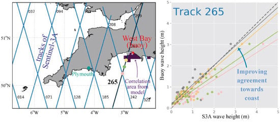
Examples of the second type of observed cahnges are from the WBy buoy shown in Figure 7. As shown in the map, both closest S3A tracks (265 and 299) cross the coastline in proximity of the buoy (∼10 and ∼30 km away, respectively). Since the coastline around the WBy buoy is quite uniform, geometrical configurations (south to southwest facing shoreline) and morphological conditions (sandy beaches) are similar at all locations. The scatter plots indicate good agreement between satellite and in-situ observations. Satellite SWH at along-track locations further offshore are higher compared with those observed by the coastal buoy. However, the two are similar at the closest locations to the buoy (and hence to the coastline) for both tracks. This is better evidenced by the regression lines, which approach the 1:1 relationship for locations progressively closer to the buoy.

Overall, the three types of behavior observed from our dataset can be visualised by plotting the regression slope as a function of the distance from each buoy (Figure 8). As already mentioned, the Hub buoy represents the only case of open sea buoy in the network analysed in our study. The associated slopes are high at all along-track locations (∼0.8 on average) and do not show any variation with respect to the distance from the buoy. The Pnz buoy represents a coastal buoy with bad agreement between in-situ and satellite observations. Similar buoys include Mhd, Plv, PtI, SMS, StB, Tor, Wey and Wst. For such buoys, regression slopes are low (<0.6) at all locations. In some cases, such as the Pnz buoy, the regression slope does not show any variation with respect to the distance from the buoy; in others (as is the case for the Tor and Wey buoys, not shown), the slope shows increasing values with decreasing distance from the buoy. Coastal buoys with good agreement between in-situ and satellite observations (such as the WBy buoy) also show low slope values at the farthest locations from the buoy. However, the values progressively increase as the along-track locations approach the buoy, until reaching values ∼1 at the closest locations. This group of buoys include Bdf, Csl, Dwl, E1, LoB and Prp.

The good agreement between in-situ and satellite observations obtained for some of the buoys indicate that S3A SAR observations can accurately retrieve SWH near the coast. Moreover, regression slope behavior such as that observed for the WBy buoy suggest that satellite observations can also correctly capture the progressive attenuation of SWH as the open ocean swells propagate towards the coast (see Figure 4 and Figure 7). However, the poor correlations observed at other coastal buoys show that this is not always the case. Those poor correlations can occur because of two reasons: (a) intrinsic inaccuracies of S3A SAR observations in coastal regions; or (b) poor pairing between the in-situ and satellite observations used for the validation. The latter case occurs when in-situ and satellite observations are compared from spatially close locations that are however representative of markedly different SWH conditions. Poor pairing could indeed be a relevant issue in our analysis since most of the SW England coast is characterised by complex morphology and conditions can rapidly vary even between close locations. Because of that, buoy-to-track distance is likely to be inadequate to identify the appropriate track–buoy combinations to be used for validation in such a complex coastal region. Thus, to better assess the nature of the observed poor correlations and identify more accurately the appropriate track–buoy combinations to validate the satellite observations, we decided to integrate in our analysis the results from the wave numerical model described in Section 2.4.

4.2. Areas of Correlation

Figure 9 shows the spatial distribution of the four parameters (correlation coefficient, regression slope, regression intercept and RMSE) derived from the WWIII-AMM7 model simulation for the Hub buoy, as described in Section 3.2. Values of the correlation coefficient ($r^2$) are larger than 0.8 over most of the model domain, indicating good linear regression between SWH time series at the Hub buoy and those from the rest of the model domain. Although not as large as for the Hub buoy, high values of $r^2$ extend for good portions of the model domain also for the rest of the coastal buoys (not shown). This is expected, since, although attenuated, SWH at the coast remains related to the SWH in the open sea. This is the reason for the high threshold value defined for $r^2$ (Section 3.2). For the regression slope parameter, the lower threshold was defined based on the average values observed from the in-situ and satellite correlations obtained for the Hub buoy (Figure 8). The upper one was then defined so that the threshold interval is symmetric around 1. Figure 9 (top) shows that for the Hub buoy a large portion of the model domain is within these thresholds. However, the areas within thresholds are more localised for the coastal buoys, indicating that the chosen values are appropriate for identifying the significant areas of similarity. Among the four parameters, RMSE is the most localised around the Hub buoy (Figure 9d) and, hence, the most restrictive in defining the area of correlation. The same occurs for all coastal buoys. The threshold value of RMSE is in line with the average values observed for traditional altimetry mission in the open ocean [10,29]. In the case of the coastal buoys, it represents roughly 25% of the observed mean SWH (∼1 m; see the time series for the WBy and Pnz buoys in Figure 3 as examples). As shown in Figure 9, despite the rapid decrease of RMSE away from the buoy, the area within the threshold still extends for several grid points around the buoy location. Finally, the regression intercept parameter shows a large area of values close to 0 in the case of the Hub buoy, but much reduced areas for the coastal buoys (similarly to what is observed for the distribution of regression slope values near 1). For those buoys, the distribution patterns of the intercept values are analogous to those observed for the RMSE. However, even for an absolute threshold value much smaller than the RMSE, the areas within the intercept thresholds are much larger than those found for the RMSE at all buoys (this also includes the Hub buoy, as shown in Figure 9c). For this reason, the intercept parameter has the least impact among the four in defining the area of correlation around each buoy.

The resulting areas of correlation for the Hub, Pnz and WBy buoys are shown in Figure 10. Comparison with Figure 9 confirms that the areal extent for the Hub buoy is most strongly constrained by the RMSE parameter (Figure 9a). The figure indicates that S3A tracks 071 and 094 can be used for comparison with in-situ observations at the Hub buoy, and that satellite observations are expected to compare well with the in-situ one along a large portion of each track near the buoy (the portion along track 071 being shorter than that along track 094). Thus, it confirms the results discussed in Section 4.1 (Figure 5). Furthermore, although not tested in our analysis, the figure suggests that in-situ observations from the Hub buoy could also be used to validate those from track 128, although the track is much further from the buoy then the two used in our analysis.

The area of correlation for the Pnz buoy (Figure 9b) is limited to two grid points near the buoy location. The main constraint for such limited extent is due to the RMSE values which rapidly increase to values >0.5 m just two grid points away from the buoy. No satellite tracks intersect this area. This indicates that the poor correlations between in-situ and satellite observations at the Pnz buoy (Figure 6) are due to poor pairing rather than inaccuracies in satellite observations. Analogous results were obtained for some of the other buoys (Mhd, Plv, SMS, StB and Wst) that showed poor correlations between in-situ and satellite observations. For the remaining three buoys (PtI, Tor and Wey), the areas of correlations indicate that satellite observations from at least one of the two closest tracks should compare well against the in-situ observations. Closer inspection of the buoy location showed that all three buoys are located very close to the coast within small bays. Because of the coarse grid resolution, these bays are not represented in the model. As a consequence, all three buoy locations correspond to land points in the model grid. To derive the area of correlation, the analysis retrieves the SWH time-series at the buoy site using SWH from the nearest ocean point in the model. However, it is likely that such points do not correctly represent the SWH conditions observed by the three buoys in much more sheltered locations. As such, we decided to not include results from those buoys in the analysis.

The area of influence for the WBy buoy is shown in Figure 10c. The figure confirms that satellite observations along the portion of track 265 closest to the buoy should be similar to the buoy observations, as shown in Figure 7 and Figure 8. At the same time, despite the good correlations obtained in Figure 7c, it indicates that satellite observations from track 299 should not be validated with the WBy observations. That track intersects the coastline immediately east of Weymouth (Wey). Again, because of the low grid resolution, fine scale coastal features (such as Weymouth Bay and the Isle of Portland immediately south of it) are only coarsely represented in the model. Therefore, it is likely that their sheltering effect on the SWH field is also misrepresented, and that coastal observations along track 299 are indeed analogous to the ones at WBy (as is the case for the model grid point immediately east of the track). For these reasons, we decided to retain track 299 in the analysis (this includes observations from the WBy buoy as well as the Csl one). Similar analysis for the other buoys which showed good correlation with satellite observations confirmed the good pairing between both closest S3A tracks and the Csl, E1 and Prp buoys. For the Bdf and Dwl buoys, the analysis indicated that only one of the two tracks should be used (185 and 242, respectively). Thus, the other two (151 and 265, respectively) were removed from the analysis. For the LoB buoy, the analysis showed that both closest tracks (185 and 208) are not representative of the conditions observed at the buoy location, and thus both pairings were removed from the analysis. Indeed, although characterised by increasing slope values with decreasing distance from the buoys (as seen for the WBy buoy, Figure 8), the four removed satellite track–buoy combinations all showed maximum slope values that remained below 0.8 even at the minimum distance from the buoy. This suggests less accurate correlations than observed for the other pairings, further supporting the results from the model analysis.

Finally, the areas of correlation around buoys LoB and StB indicated that tracks different from the two closest ones should be used. This further confirms that, in a complex coastal environment such as southwest England, the distance from the buoy alone is not a reliable parameter to define the appropriate wave buoys to be used for validating satellite observations along specific tracks. The new tracks correspond to track 128 for the LoB buoy, and to track 242 for the StB one. These two new pairings were included in the analysis.

The final buoy–S3A track pairings are summarised in

Table 2. List of buoy–track parings used in Section 4.3 to evaluate S3A performance in the coastal zone. In bold are the tracks identified using the area of correlation described in Section 4.2.

Buoy	S3A Tracks
Bdf	185	–
Csl	265	299
Dwl	242	–
E1	185	208
LoB	128	–
Prp	128	151
StB	242	–
WBy	265	299

and illustrated in Figure 11. (The Hub buoy is not considered in the subsequent analysis, as it is effectively open ocean rather than coastal.) Sensitivity analysis on the identification of the area of correlation showed that relaxing the thresholds for the four parameters modified the extent of the areas but did not substantially change the identified pairs for each buoy. These pairs are used in the next section to evaluate the performance of S3A SWH observations in our coastal region.

4.3. Evaluation of S3A Performance in the Coastal Region

Figure 12 shows the regression slope and the RMSE between S3A and in-situ SWH observations as a function of the distance from each buoy for the pairings listed on Table 2. Both diagnostics indicate good performance of satellite SAR observations in the coastal zone. The regression slope (Figure 12a) shows an inverse relation with respect to the distance from the buoy, with slope values approaching the 1:1 relation as satellite measurements are collected progressively closer to the buoys. The RMSE decreases from values of about 1 m at 60 km from the buoys to less than 0.5 m at 30 km. For closer distances to the buoys, the RMSE remains bound between values of 0.6 and 0.25 m.

As none of the buoys is positioned directly under a S3A track, the minimum distance between buoy and satellite observations is never below ∼10 km, even for the closest pairings. For some pairings (e.g., Wby–299, Csl–265 and E1–185) the minimum distance is on the order of 30 km, and for others (e.g., LoB–128 and PrP–151) even more. Moreover, under certain geometrical conditions (such as in the case of the Stb–242 pairing), the closest position to the buoy along a satellite track can correspond to a location that is further offshore than the buoy. Because of that, the closest regression slopes to the 1:1 relation can be found at locations more representative of the same coastal conditions found at the buoy location, but further away from the buoy than the closest ones. Thus, as in the case of the pairing selection in Section 4.2, even in this case the distance from the buoy is not the most appropriate variable to be used for the analysis.

Alternatively, the regression slopes can also be plotted as a function of the distance from the coast (Figure 13a). In this case, the slopes still show the same inverse correlation as in Figure 12a. Moreover, the closest values to 1 occur at the minimum distance from the coast for almost all pairings. Exceptions are the E1–208, LoB–128 and Bdf–185 pairings. E1 represents a special case with respect to the other buoys included in the analysis, since it is located in deeper waters and further away from the coast. For this reason, the closest regression slope to the 1:1 relation occurs at about 20 km from the coast, whereas as expected it increases to about 1.2 within 5 km from the coast (i.e., satellite observes smaller SWH values near the coast than those at E1). Regarding the Lob and Bdf buoys, their regression slopes increase with decreasing distance from the coast down to 10 km, but they maintain similar values for the closest points to the coast. Since the satellite tracks associated with both buoys intersect the coast in areas characterised by complex morphology and small bays, it is possible that the coarse resolution of the numerical model leads to inaccurate results in the identification of the area within which satellite observations can be paired with the two buoys. Finally, Dwl–242 is the only other satellite track–buoy pairing that does not show a regression slope above 0.8. As opposed to LoB and Bdf, the buoy is located on a portion of the coast where other buoys show very good correlation with the associated satellite measurements (e.g., StB, Wby and Csl). Thus, coarse model resolution cannot be hypothesised to be the cause for such low regression slopes, and the reasons for the poor performances observed at Dwl remain to be determined.

Regression slopes from PLRM observations (Figure 13b) show worse performance than those from SAR. These regression values are still characterised by a trend towards the 1:1 relation as the distance from the coast decreases down to 15 km. However, they have a broader range of values than SAR at similar distances. Furthermore, the regression slopes quickly decrease to very low values within 15 km from the coast, indicating that in that region PLRM SWH observations are consistently larger than those observed by the buoys. Such high PLRM-based SWH observations are likely resulting from retracking errors due to contaminations in the returned echoes by the presence of land within the satellite footprint near the coast.

Figure 14 shows the RMSE for SAR and PLRM observations as a function of distance from the coast. While RMSE values of SAR observations (Figure 14a) remain inversely correlated with the distance from the coast, their decrease approaching the coast is less pronounced compared with Figure 12b. The average value within 15 km from the coastline is $0.46\pm 0.14$ m, while offshore of 15 km it is $0.60\pm 0.22$ m. RMSE values of PLRM observations (Figure 12b) show trend and values similar to SAR offshore of 15 km (average value is $0.63\pm 0.23$ m). However, they quickly degrade within 15 km from the coast (average value $0.84\pm 0.45$ m), with particularly larger errors when the coast is within 5 km. Thus, as for the regression slope, SAR observations outperform PLRM ones in the coastal region also in terms of RMSE.

To better understand whether some geophysical factors can potentially contribute to the observed RMSE in SAR mode, we investigated the dependence of the bias between satellite and in-situ observation on the swell characteristics. Figure 15 shows the difference between satellite and buoy observations as function of the swell period for each of the pairings from Table 2. Each point represents the difference of a given satellite observation at the location closest to the coast. The resulting distribution does not evidence any trend or correlation between bias and swell period (an analogous distribution was also obtained for PLRM observations; not shown). Thus, no clear dependence between the two can be identified from our analysis.

The same biases were also analysed as a function of the swell direction to assess their dependence on the relative incident angle between swell and satellite track. The polar plots in Figure 16 show the difference between satellite and buoy observations as a function of swell direction for each satellite track associated with the buoys WBy, E1 and PrP. For each buoy, no clear trends or patterns can be identified in the distributions of the bias either as a function of varying swell directions for a given satellite track, or as a function of different satellite tracks for the same swell direction. An exception is represented by the E1 buoy that shows larger biases along track 208 than along track 185 for swells directions between W and SW. However, this is the only example among all the pairings from Table 2. Thus, as in the case of swell period, no clear dependence between the observed bias and swell direction can be identified from our analysis.

Previous studies based on sea level anomaly has also shown a dependency on altimetry performance based on whether the satellite transition is from sea to land or vice versa. Unfortunately, within our dataset, there are only three buoys paired with satellite tracks with both types of transition: Prp, WBy and Csl (the latter two being very close to each other and paired with the same satellite tracks). With such limited number of observations, it was not possible to identify an analogous dependency of SWH on satellite track transition.

5. Discussion

The first step of our analysis was to implement an automated method to identify which satellite observations could be compared against the observations from each buoy. Our initial approach was to use the distance between buoy locations and satellite tracks as an objective diagnostic to identify the appropriate track–buoy pairings to be used for the validation. While such a diagnostic can be successfully used in the open ocean (where the characteristics of the wave field change gradually and over larger spatial scales), it showed some limitations in our region of study (where wave height and direction can change drastically over short distances along the coast due to wave interactions with land and bathymetry). A second approach involved the use of wave fields from a regional numerical model to identify the areas around each buoy location where wave characteristics are expected to remain similar. In the text, we refer to such areas as “areas of correlation”. After those regions were defined, in-situ observations from a given buoy were compared only with satellite observations collected within its corresponding area of correlation. This second approach was better suited to identify the appropriate satellite–buoy parings to be used for the validation.

Comparison with the buoy observations indicated good performance of S3A SAR observations of SWH near the coast. S3A shows decreasing SWH for observations progressively closer to the coast, consistent with what is expected from theory and predicted by numerical models. Thus, correlations with the coastal buoy observations are characterised by an inverse relation with respect to distance from the coast. Regression slopes are between 0.6 and 0.2 at more than 30 km from the coast and progressively increase towards 1 for closer and closer distances. For most of the buoys, the regression slopes closest to the 1:1 relation occur at the minimum distance from the coast. On the contrary, regression slopes based on PLRM observations show a sharp decrease to values between 0.8 and 0.1 within the last 15 km from the coast. Improved performance of SAR observations with respect to PLRM were also observed from the analysis of RMSE as function of distance from the coast. Average value of RMSE within 15 km from the coast was found to be $0.46\pm 0.14$ m for SAR observations and $0.84\pm 0.45$ m for PLRM. Thus, our analysis confirms the expected advantages of SAR altimetry over traditional nadir altimetry in coastal regions. For conventional LRM mode altimeters, differences in the quality of range data have been noted between tracks approaching and receding from land; it was not possible to identify such distinction in our dataset for SWH data from a SAR-mode instrument.

Dependence of the bias between satellite and in-situ observations on swell characteristics was also explored. However, our analysis could not identify any correlation or trend between the observed biases and swell period or direction. Prior work had shown that the thin rectangular instrument footprint associated with SAR processing can sometimes lead to an underestimate of SWH [20]; we surmise that our results differ because even the data from the buoys well exposed to the North Atlantic did not observe sufficiently long wavelength swell at the time of our S3A overpasses.

Many recent studies have focussed on improving performance of traditional nadir altimetry over coastal regions by developing and assessing dedicated coastal retracking algorithms [6,17,18]. There is the potential that some of these algorithms could be adapted to improve wave height estimates from S3A PLRM in the coastal zone, making use of appropriate quality control of the data. As SAR mode altimetry over the ocean is still new, there is also much scope for innovative algorithms to optimise SWH retrieval in the coastal zone.

6. Conclusions

In this study, we assessed the performance of S3A SAR observations in the coastal region of southwest England using in-situ observations from an array of 17 coastal wave buoys. The analysis indicates that SAR observations outperform PLRM within 15 km from the coast. Within that region, regression slopes between SAR and buoy observations are close to the 1:1 relation, and the average root mean square error between the two is $0.46\pm 0.14$ m. On the other hand, regression slopes for PLRM observations rapidly deviate from the 1:1 relation, while the average root mean square error increases to $0.84\pm 0.45$ m. The analysis did not identify any dependence of the bias between SAR and in-situ observation on the swell period or direction.

The validation approach outlined in this paper combines satellite and in-situ observations with numerical model results. Its general, principles have been designed with the aim of implementing a validation analysis for complex coastal regions that is as automated as possible. One obvious advantage of such an approach is that it can be easily applied to different regions and/or altimeters. Due mainly to the coarse resolution of the wave numerical model adopted in this study, our analysis still required a certain degree of manual intervention to correctly identify the appropriate satellite–buoy pairings to be used for validation. However, higher resolution models should drastically reduce the need for manual intervention. As such, we are confident that the proposed validation approach could be successfully replicated in future studies to assess the performance of Sentinel-3B in southwest England as well as to extend the assessment of S3A SAR performance over additional coastal regions spanning an even broader range of swell characteristics and conditions.

References

1. Ardhuin, F.; Stopa, J.E.; Chapron, B.; Collard, F.; Husson, R.; Jensen, R.E.; Johannessen, J.; Mouche, A.; Passaro, M.; Quartly, G.D.; et al. Observing Sea States. Front. Mar. Sci. 2019, 6, 124. [Google Scholar] [CrossRef] [Green Version]
2. Cronin, M.F.; Gentemann, C.L.; Edson, J.; Ueki, I.; Bourassa, M.; Brown, S.; Clayson, C.A.; Fairall, C.W.; Farrar, J.T.; Gille, S.T.; et al. Air-Sea Fluxes With a Focus on Heat and Momentum. Front. Mar. Sci. 2019, 6, 430. [Google Scholar] [CrossRef] [Green Version]
3. D’Asaro, E.A. Turbulence in the Upper-Ocean Mixed Layer. Annu. Rev. Mar. Sci. 2014, 6, 101–115. [Google Scholar] [CrossRef] [PubMed]
4. Young, I.R.; Ribal, A. Multiplatform evaluation of global trends in wind speed and wave height. Science 2019, 364, 548–552. [Google Scholar] [CrossRef]
5. Bailey, K.; Steinberg, C.; Davies, C.; Galibert, G.; Hidas, M.; McManus, M.A.; Murphy, T.; Newton, J.; Roughan, M.; Schaeffer, A. Coastal Mooring Observing Networks and Their Data Products: Recommendations for the Next Decade. Front. Mar. Sci. 2019, 6, 180. [Google Scholar] [CrossRef] [Green Version]
6. Passaro, M.; Fenoglio-Marc, L.; Cipollini, P. Validation of Significant Wave Height From Improved Satellite Altimetry in the German Bight. IEEE Trans. Geosci. Remote Sens. 2015, 53, 2146–2156. [Google Scholar] [CrossRef]
7. Le Traon, P.Y. From satellite altimetry to Argo and operational oceanography: Three revolutions in oceanography. Ocean Sci. 2013, 9, 901–915. [Google Scholar] [CrossRef] [Green Version]
8. Gommenginger, C.; Thibaut, P.; Fenoglio-Marc, L.; Quartly, G.; Deng, X.; Gomez-Enri, J.; Challenor, P.; Gao, Y. Retracking altimeter waveforms near the coasts. In Coastal Altimetry; Vignudelli, S., Kostianoy, A.G., Cipollini, P., Benveniste, J., Eds.; Springer: Berlin/Heidelberg, Germany, 2011; pp. 61–102. [Google Scholar]
9. Brown, G. The average impulse response of a rough surface and its applications. IEEE Trans. Antennas Propag. 1977, 25, 67–74. [Google Scholar] [CrossRef]
10. Durrant, T.H.; Greenslade, D.J.M.; Simmonds, I. Validation of Jason-1 and Envisat Remotely Sensed Wave Heights. J. Atmos. Ocean. Technol. 2009, 26, 123–134. [Google Scholar] [CrossRef]
11. Chelton, D.B.; Walsh, E.J.; MacArthur, J.L. Pulse Compression and Sea Level Tracking in Satellite Altimetry. J. Atmos. Ocean. Technol. 1989, 6, 407–438. [Google Scholar] [CrossRef] [Green Version]
12. Cotton, P.D.; Carter, D.J.T. Cross calibration of TOPEX, ERS-I, and Geosat wave heights. J. Geophys. Res. Ocean 1994, 99, 25025–25033. [Google Scholar] [CrossRef]
13. Young, I. An intercomparison of GEOSAT, TOPEX and ERS1 measurements of wind speed and wave height. Ocean. Eng. 1998, 26, 67–81. [Google Scholar] [CrossRef]
14. Zieger, S.; Vinoth, J.; Young, I.R. Joint Calibration of Multiplatform Altimeter Measurements of Wind Speed and Wave Height over the Past 20 Years. J. Atmos. Ocean. Technol. 2009, 26, 2549–2564. [Google Scholar] [CrossRef]
15. Gomez-Enri, J.; Vignudelli, S.; Quartly, G.D.; Gommenginger, C.P.; Cipollini, P.; Challenor, P.G.; Benveniste, J. Modeling Envisat RA-2 Waveforms in the Coastal Zone: Case Study of Calm Water Contamination. IEEE Geosci. Remote. Sens. Lett. 2010, 7, 474–478. [Google Scholar] [CrossRef]
16. Wang, X.; Ichikawa, K. Coastal waveform retracking for Jason-2 altimeter data based on along-track Echograms around the Tsushima Islands in Japan. Remote Sens. 2017, 9, 762. [Google Scholar] [CrossRef] [Green Version]
17. Hithin, N.K.; Remya, P.G.; Balakrishnan Nair, T.M.; Harikumar, R.; Kumar, R.; Nayak, S. Validation and Intercomparison of SARAL/AltiKa and PISTACH-Derived Coastal Wave Heights Using In-Situ Measurements. IEEE J. Sel. Top. Appl. Earth Obs. Remote. Sens. 2015, 8, 4120–4129. [Google Scholar] [CrossRef]
18. Peng, F.; Deng, X. Validation of Improved Significant Wave Heights from the Brown-Peaky (BP) Retracker along the East Coast of Australia. Remote Sens. 2018, 10, 1072. [Google Scholar] [CrossRef] [Green Version]
19. Raney, R.K. The delay/Doppler radar altimeter. IEEE Trans. Geosci. Remote. Sens. 1998, 36, 1578–1588. [Google Scholar] [CrossRef]
20. Moreau, T.; Tran, N.; Aublanc, J.; Tison, C.; Gac, S.L.; Boy, F. Impact of long ocean waves on wave height retrieval from SAR altimetry data. Adv. Space Res. 2018, 62, 1434–1444. [Google Scholar] [CrossRef]
21. Raynal, M.; Labroue, S.; Moreau, T.; Boy, F.; Picot, N. From conventional to Delay Doppler altimetry: A demonstration of continuity and improvements with the Cryosat-2 mission. Adv. Space Res. 2018, 62, 1564–1575. [Google Scholar] [CrossRef]
22. Wingham, D.; Francis, C.; Baker, S.; Bouzinac, C.; Brockley, D.; Cullen, R.; de Chateau-Thierry, P.; Laxon, S.; Mallow, U.; Mavrocordatos, C.; et al. CryoSat: A mission to determine the fluctuations in Earth’s land and marine ice fields. Adv. Space Res. 2006, 37, 841–871, Natural Hazards and Oceanographic Processes from Satellite Data. [Google Scholar] [CrossRef]
23. Fenoglio-Marc, L.; Dinardo, S.; Scharroo, R.; Roland, A.; Sikiric, M.D.; Lucas, B.; Becker, M.; Benveniste, J.; Weiss, R. The German Bight: A validation of CryoSat-2 altimeter data in SAR mode. Adv. Space Res. 2015, 55, 2641–2656. [Google Scholar] [CrossRef]
24. Boy, F.; Desjonquères, J.; Picot, N.; Moreau, T.; Raynal, M. CryoSat-2 SAR-Mode Over Oceans: Processing Methods, Global Assessment, and Benefits. IEEE Trans. Geosci. Remote. Sens. 2017, 55, 148–158. [Google Scholar] [CrossRef]
25. Wiese, A.; Staneva, J.; Schulz-Stellenfleth, J.; Behrens, A.; Fenoglio-Marc, L.; Bidlot, J.R. Synergy of wind wave model simulations and satellite observations during extreme events. Ocean Sci. 2018, 14, 1503–1521. [Google Scholar] [CrossRef] [Green Version]
26. Scott, T.; Masselink, G.; Russell, P. Morphodynamic characteristics and classification of beaches in England and Wales. Mar. Geol. 2011, 286, 1–20. [Google Scholar] [CrossRef] [Green Version]
27. Smyth, T.; Atkinson, A.; Widdicombe, S.; Frost, M.; Allen, I.; Fishwick, J.; Queiros, A.; Sims, D.; Barange, M. The Western Channel Observatory. Prog. Oceanogr. 2015, 137, 335–341. [Google Scholar] [CrossRef]
28. Sen, P.K. Estimates of the Regression Coefficient Based on Kendall’s Tau. J. Am. Stat. Assoc. 1968, 63, 1379–1389. [Google Scholar] [CrossRef]
29. Ray, R.D.; Beckley, B.D. Calibration of Ocean Wave Measurements by the TOPEX, Jason-1, and Jason-2 Satellites. Mar. Geod. 2012, 35, 238–257. [Google Scholar] [CrossRef]
Figure 1. Locations of S3A tracks (blue lines) and wave buoys (red dots) used for this study.
Remotesensing 11 02998 g001
Figure 2. SWH along track 128 for cycle 6: (a) PLRM; and (b) SAR mode. The gap in both tracks is due to land. In orange are the data averaged with a moving Gaussian window of 50 samples at FWHM (corresponding to σ 21 samples).
Remotesensing 11 02998 g002
Figure 3. (a,d,g) Locations of the Hub, WBy and Pnz buoys (red circles). Each displayed area extends for ∼15 km on all sides of the relevant buoy. (b,e,h) Time series of SWH for the three buoys. (c,f,i) Polar distribution of observed principal wave direction and period for the three buoys.
Remotesensing 11 02998 g003
Figure 4. Example of significant wave height (colour) and swell direction (streamlines) from the WWIII-AMM7 model for 15 February 2018 at 01:00.
Remotesensing 11 02998 g004
Figure 5. (a) Map showing the Hub buoy position (magenta star), the two nearest S3A tracks to the buoy (tracks 094 and 071, both in blue) and the various locations along each track at which the correlations between satellite and in-situ observations were computed (coloured circles and triangles). (b,c) Scatter plots between S3A SAR and in-situ observations at each location (symbols and colours are the same as in panel (a)) and corresponding regression lines. The gray dashed line indicates the 1:1 relationship.
Remotesensing 11 02998 g005
Figure 6. Same as Figure 5 but for the Pnz buoy and S3A tracks 071 and 094.
Remotesensing 11 02998 g006
Figure 7. Same as Figure 5 but for the WBy buoy and S3A tracks 265 and 299.
Remotesensing 11 02998 g007
Figure 8. Variation of the regression slope as function of the distance from the buoy for the Hub, Pnz and WBy buoys. The regression slopes were computed at varying locations along the two closest S3A tracks to each buoy.
Remotesensing 11 02998 g008
Figure 9. Example of spatial distribution of the correlation coefficient (a), regression slope (b), regression intercept (c) and RMSE (d) computed between the time series of the WWIII-AMM7 model simulation nearest to the Hub buoy and those at each of the grid points of the model domain (see Section 3.2 for more details). The red circle marks the position of the Hub buoy. The thicker contours mark the thresholds for each parameter used to define the areas of correlation around each buoy shown in Figure 10: correlation coefficient ( r 2 ) 0.95 , 0.8 slope 1.2 , 0.1 m intercept 0.1 m and RMSE 0.25 m.
Remotesensing 11 02998 g009
Figure 10. Examples of areas of correlation retrieved from the model output for the Hub (a), Pnz (b) and WBy (c) buoys.
Remotesensing 11 02998 g010
Figure 11. Same as Figure 1, but showing only the wave-buoys and satellite tracks from Table 2 used for the analysis of S3A performance. The green arrows indicate approximately where along each track lie the minima of RMSE with respect to the buoy measurements.
Remotesensing 11 02998 g011
Figure 12. Correlation slope (a) and RMSE (b) between S3A and in-situ observations as function of distance between along-track location and buoy position. Only the satellite–buoy pairings from Table 2 are included. Both panels are for SAR observations.
Remotesensing 11 02998 g012
Figure 13. Regression slope between S3A and in-situ observations as a function of the distance from the coast (a) SAR observations; and (b) PLRM observations. As for Figure 12, only satellite track–buoy pairings from Table 2 are included.
Remotesensing 11 02998 g013
Figure 14. RMSE between S3A and in-situ observations as a function of the distance from the coast: (a) SAR observations; and (b) PLRM observations. As for Figure 12, only satellite track–buoy pairings from Table 2 are included.
Remotesensing 11 02998 g014
Figure 15. SWH difference between S3A SAR and in-situ observations as a function of swell period. Only the pairing from Table 2 are included. Each point is the bias computed for a given S3A cycle at the location closest to the coast for a specific track–buoy pairing.
Remotesensing 11 02998 g015
Figure 16. Polar plots with SWH difference between S3A SAR and in-situ observations as a function of swell direction for the WBy, E1, and Prp buoys. The bias varies along the radial direction from −2 m at the center to 2 m along the outermost circle. The thicker circle marks zero bias.
Remotesensing 11 02998 g016