Evaluation of HY-2A Scatterometer Ocean Surface Wind Data during 2012–2018

Abstract

This study focuses on the evaluation of global Haiyang-2A satellite scatterometer (HSCAT) operational wind products from 2012 to 2018. In order to evaluate HSCAT winds, HSCAT operational wind products were collocated with buoy measurements and rainfall data. Error varieties under different atmospheric stratification and rainfall conditions were taken into consideration. After data quality control, the average bias and root mean square error (RMSE) between buoys and HSCAT data were 0.1 m/s and 1.3 m/s for wind speed, and 1° and 27° for wind direction, respectively. Especially, the varieties of the wind direction difference change a lot under non-neutral atmospheric conditions. HSCAT wind speeds are overestimated with an increasing rainfall rate while wind directions tend to be perpendicular to buoys’. In brief, the HSCAT wind product qualities are not stable during 2012 to 2018, especially for the data in 2015 and 2016. Atmospheric stratification and rain effects should be considered in wind retrieval and marine application.

1. Introduction

The sea surface wind field is one of the direct factors affecting small-scale and large-scale seawater movement and plays an important role in marine environmental monitoring, weather forecasting, as well as other marine and atmospheric sciences studies. Owing to the spatial and temporal constraints, traditional wind measurement methods, such as ships, buoys, weather stations, and other in situ observations, are not satisfied with the requirements of high-quality and continuous wind observations for ocean research. Since the 1970s, satellite observations have become an indispensable approach to collect sea surface wind field data [1].

There are four main satellite microwave sensors for observing the global sea surface winds: Microwave scatterometer, microwave radiometer, altimeter, and synthetic aperture radar [1]. The microwave scatterometer is the main sensor for providing wind data with its all-weather and all-time capacity [2]. The earliest satellite scatterometer is the Ku-band fan beam Seasat-A Satellite Scatterometer (SASS), launched by National Aeronautics and Space Administration (NASA) in 1978. SASS opened a new era of satellite-observing sea surface wind fields [3]. Afterwards, series C-band and Ku-band scatterometers were successfully launched [4,5,6,7,8,9]. The Ku-band scatterometer of the first Chinese microwave ocean environment satellite Haiyang-2A (HSCAT), launched on 16 August 2011, is a pencil beam scatterometer with a 1700-km swath and 25-km spatial resolution [10].

Evaluating the quality of scatterometer data is indispensable for sea surface wind field study. There are abundant evaluation investigations of different sensors studied by worldwide researchers. Masuko et al. (2000) evaluated NSCAT wind vectors with Japan Meteorological Agency (JMA) buoys, National Space Development Agency of Japan (NASDA) buoys, and six JMA research vessels in the seas around Japan. They found that no significant systematic errors with wind speeds and incidence angles exist for NSCAT wind products [11]. Ebuchi et al. (2002) compared QuikSCAT/SeaWinds winds with buoy data from National Data Buoy Center (NDBC), Tropical Atmosphere Ocean (TAO), Pilot Research Moored Array in the Tropical Atlantic (PIRATA) projects, and the Japan Meteorological Agency (JMA). They found that a weak positive correlation exists between wind speed bias and significant wave height but no significant correlation with sea surface temperature or atmospheric stability [12]. Pickett et al. (2003) compared QuikSCAT with 12 nearshore and 3 offshore buoys along U.S. West Coast, and found that root mean square errors (RMSEs) of the QuikSCAT wind speed and direction were 1.3 m/s and 26°. QuikSCAT data could satisfy coastal studies although the nearshore data were less accurate than offshore data [13]. Tang et al. (2004) reproduced high-resolution QuikSCAT wind data and compared them with NDBC buoy data in coastal regions. The results showed that the modified algorithm could improve the accuracy of nearshore data, especially the accuracy of wind direction [14]. Ebuchi (2005) compared ADEOS-II SeaWinds with AMSR wind speeds and found that SeaWinds data could better match aircraft flights and other platforms data [15]. Satheesan et al. (2007) compared QuikSCAT with buoy data in the Indian Ocean. Their results showed that the consistencies in the North Indian Ocean were better than in the Equatorial Indian Ocean. Under different sea surface temperatures, QuikSCAT wind speed was generally higher, which might be due to the low accuracy at low speeds and rain contamination [16]. Yang et al. (2011) intercompared wind data from ENVISAT Advanced Synthetic Aperture Radar (ASAR), ASCAT, NDBC buoys, and the U.S. Navy Operational Global Atmospheric Prediction System (NOGAPS) model. They found ASAR data had a similar accuracy with ASCAT and NOGAPS model data, and the differences between ASCAT and ASAR-averaged wind data at different spatial resolutions changed little [17]. Sudha et al. (2013) compared OSCAT winds with buoy data and found that the OSCAT wind direction accuracy could not satisfy the mission requirements (20°) but wind direction biases decreased as speeds increased [18]. Wang et al. (2013) validated the first six months of HSCAT wind products by using NDBC buoys, R/V Polarstern, Aurora Australis, Roger Revelle (R/Vs), and PY30-1 oil platforms measurements. The RMSEs were 1.3 m/s and 19.19° compared with NDBC buoys. Similar results were also shown in R/Vs and oil platforms’ comparisons. These results verified the practicability of HSCAT wind products in marine research [19]. Xing et al. (2016) also validated HSCAT wind products by using NDBC buoys, TAO, the European Centre for Medium Range Weather Forecasting (ECMWF) reanalysis data (ERA-Interim), and ASCAT data during 2012–2014. They found that rain has a significant effect on overestimating HSCAT wind speed at low and moderate wind speeds [20]. Bhaskar et al. (2016) generated and evaluated two-day OSCAT wind fields with tropical Indian Ocean buoys and ASCAT data [21]. Lindsley et al. (2016) applied an ultrahigh resolution (UHR) to the ASCAT wind product and compared ASCAT UHR winds with standard 25-km Level-2 ASCAT winds, near-coastal buoy winds, and open ocean SAR winds. The results showed that UHR product agrees well with these products and indicated that ASCAT UHR products may be used in near coastal and storm research [22]. Verhoef et al. (2017) evaluated long-term SeaWinds and ASCAT wind datasets with buoy and numerical weather prediction (NWP) winds. They found that SeaWinds and ASCAT wind had strong stability over time [23]. Wentz et al. (2017) introduced ocean wind consistent climate data records (OW-CDRs) and mentioned four evaluation methods, including a comparison with buoy winds, comparison with numerical model winds, comparison between two different platform sensors, and comparison between different data providers. They also planned some methods of calibrating other instruments, which would be merged into OW-CDRs in the future [24].Yang et al. (2018) evaluated ISS-RapidScat wind vectors by using various buoys and ASCAT data. The average biases of ISS-RapidScat winds were 1.42 m/s and 19.5° compared with buoys while the biases were 1.15 m/s and 15.21° compared with ASCAT [9]. Hutchings et al. (2019) applied direction interval retrieval techniques and other processing improvements to RapidScat 2.5-km ultrahigh-resolution (UHR) winds. They also validated the new products with Level 2B (L2B) winds, numerical weather prediction winds, and buoy winds. The results showed that the new retrieval algorithm can improve the spatial consistency of UHR winds [25].

At present, studies of satellite scatterometer wind field evaluation are mostly regional and in a short-time period. Our research focused on a global and long-term evaluation to study the stability of the HSCAT-operated wind product during 2012–2018. Additionally, atmospheric stratification and rain effects on scatterometer wind retrieval were taken into account.

In this paper, we used HSCAT operational Level 2B wind products from January 2012 to December 2018 and buoy data provided by the European Centre for Medium-Range Weather Forecasts (ECMWF) MARS archive to evaluate and analyze HSCAT wind products. In addition, we also combined HSCAT data with the Special Sensor Microwave Imager Sounder (SSMIS) rainfall data to evaluate the rain effects on HSCAT winds. Scatterometer winds, buoy winds, and SSMIS rainfall data as well as their collocation methods are introduced in Section 2; the main product analysis, atmospheric stratification, and rain effect results are discussed in Section 3; and summaries of this study are provided in Section 4.

2. Data and Data Collection

2.1. HSCAT Data

Haiyang-2A (HY-2A) satellite is the first Chinese microwave ocean environment satellite launched by National Satellite Ocean Application Service (NSOAS) on 16 August 2011. HY-2A is sun-synchronous with a 971-km orbital altitude. Detailed information of the HY-2A satellite is shown in

Table 1. Haiyang-2A (HY-2A) satellite parameters.

HY-2A Satellite Parameters	Description
Orbit	Sun-synchronous Orbit
Orbital Altitude	971 km
Orbital Inclination	99.34°
Local Time of Descending Node	6:00 a.m.
Repetition (Earlier Stage)	104.46 min
Laps (Earlier Stage)	13+11/14 times
Repetition (Later Stage)	104.50 min
Laps (Later Stage)	13+131/168 times
Instruments	Radar Altimeter; Microwave Scatterometer; Microwave Radiometer; DORIS; GPS; Laser Range Finder

[10]. The Ku-band scatterometer on HY-2A (HSCAT) operates at 13.3 GHz with the pencil beam conical scanning mode. The inner antenna works in horizontal polarization (HH) at a 41° incidence angel over a 1350-km swath, and the outer antenna works in vertical polarization (VV) at a 48° incidence angel over a 1700-km swath. HSCAT Level 2B (L2B) wind vectors are retrieved based on NSCAT-2 Geophysical Model Function (GMF) by maximum likelihood estimation (MLE) and the circle median filter is used to remove wind direction ambiguities [26]. The L2B products provide daily sea surface information in orbits with a 25-km resolution, and every single data file consists of 1624 rows and 76 columns. The wind direction in L2B products is defined as 0 degrees when wind is blowing toward the north and increases in the clockwise [27]. The HSCAT L2B wind data from 2012 to 2018 were used in this paper.

2.2. ECMWF MARS Buoy Data

In situ wind observations are used to evaluate HSCAT winds. Buoy wind vectors are distributed by the Global Telecommunication System (GTS), which have been retrieved and quality controlled by the ECMWF MARS archive. The temporal resolution of buoy winds is one hour by averaging the wind data over 10 min. The wind direction is defined as 0 degrees when wind is blowing from north and increases in the clockwise direction [23]. The data of 248 buoy stations consisting of 30 nearshore buoy stations (within 50 km from the coast) and 218 offshore stations (more than 50 km away from the coast) were collected in this study and their locations are shown in Figure 1.

As scatterometer wind data are regarded as 10-m neutrally stable wind, all buoy winds were converted to 10-m neutral winds (marked as $\overrightarrow{V_{10n}}$) by using the LKB model proposed by Liu, Katsaros and Businger in 1979 [28,29]. However, the scatterometer measures the sea surface normalized radar cross-section (NRCS), which is affected by wind friction directly. Therefore, we converted $\overrightarrow{V_{10n}}$ to stress-equivalent wind (marked as $\overrightarrow{V_{10s}}$). The relation between the stress-equivalent wind and neutral winds is [30]:

$$\overrightarrow{V_{10s}}=\overrightarrow{V_{10n}}\sqrt{\frac{\rho }{\langle \rho \rangle }},$$

(1)

where $\rho$ is the air density (kg/m³); and $\langle \rho \rangle$ is the global average air density and equals to 1.225 kg/m³ here.

2.3. SSMIS Data

To study rain effects on HSCAT wind retrieval, we used the Special Sensor Microwave Imager Sounder (SSMIS) rainfall data to extract HSCAT wind data contaminated by rain. The Special Sensor Microwave Imager (SSM/I) and SSMIS are series microwave radiometers payloaded on the near-polar orbiting Defense Meteorological Satellite Program (DMSP) satellites since 1987. SSMIS works at 19.35, 22.235, 37, and 85.5 GHz. The rainfall data are provided with a gridded dataset of a 0.25° spatial resolution generated by Remote Sensing System (REMSS) [31]. To match with the HSCAT descending time, we chose the DMSP F17 platform, of which the descending time (6:37 a.m.) is the closest to HSCAT’s (6:00 a.m.) and quite stable during the chosen time period. The ascending and descending equatorial crossing time for different instruments can be inquired from REMSS [32].

2.4. Data Collocation Method

Before collocation, data selection and quality control need to be done firstly. Because of the dependences between the azimuth dispersion of rotating scan scatterometer and the accuracies of wind vector retrieval, small azimuth dispersion causes a lower quality in the winds [33,34,35]. Cross-track wind cell can be divided as the outer swath (OS, or outer region (OR)) and inner swath (IS) and IS consists of a sweet region (SR) and nadir region (NR), as shown in Figure 2. Since only vertical polarization exists in the outside edge region of the swath, HSCAT OS data were not included in the collocation dataset. For buoy data, some of the buoys changed their moored locations during measurement. We selected the buoy data measured at the same time but with different locations, and averaged the buoy data as one measurement. As for SSMIS rainfall data, we removed all the invalid data marked by REMSS.

After data quality control, we made the buoy and scatterometer collocation datasets first. HSCAT wind field data and buoy wind data were collocated within $25/\sqrt{2}$ km (about 17.7 km) and 30 min. In this study, wind speeds were used within 0.1 to 25 m/s and HSCAT wind directions were turned 180° to keep with the buoy wind directions before analysis. As for rainfall data, we used the location of HSCAT wind data to find F17 SSMIS rain data within 1 h.

Due to the sea surface status being affected by the terrain in shallow water and the contamination of the island, NRCS is greatly affected near the coast. We classified buoy data as the offshore dataset and nearshore dataset according to the distance between buoy stations and coastline. There are 30 nearshore buoy stations within 50 km from the coastline and others are offshore buoy stations, as shown in Figure 1. Besides, it was found that the amount of nearshore data is about 4% of the offshore data. RMSEs of the nearshore data were about 1.58 m/s and 35.52°while the results of the offshore data were 1.30 m/s and 27.40°during the whole study period. The deviation of the nearshore data is large and therefore only the offshore dataset was used in this study.

3. Results and Discussions

3.1. Statistical Analysis of HSCAT Wind Variations from 2012 to 2018 Year by Year

To evaluate the quality of the HSCAT wind data, HSCAT winds were collocated with buoy data year by year from 2012 to 2018. The spatial-temporal collocation windows are 17.7 km and 30 min as introduced in Section 2.

3.1.1. The Distribution of Collocated Data and Statistical Parameters

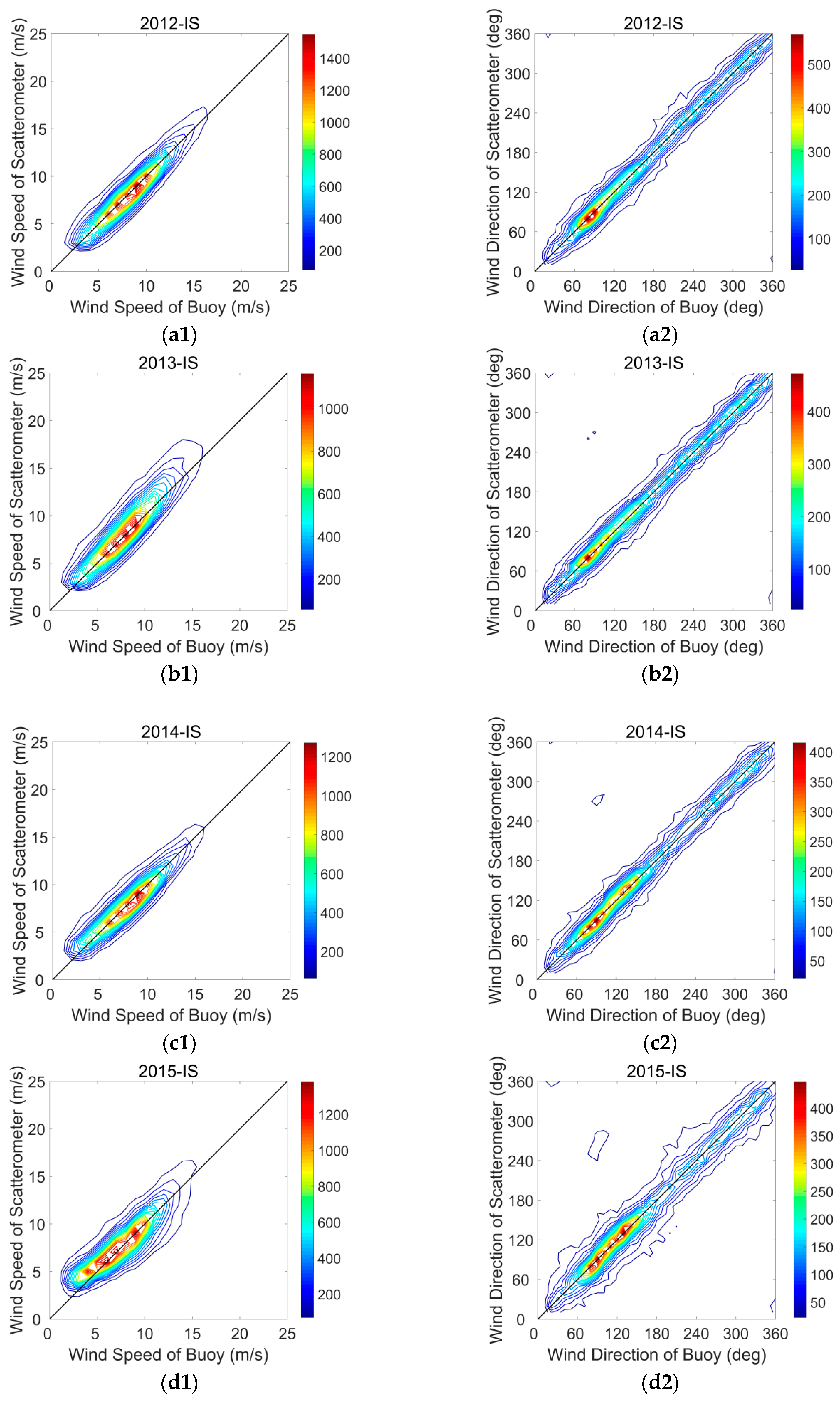
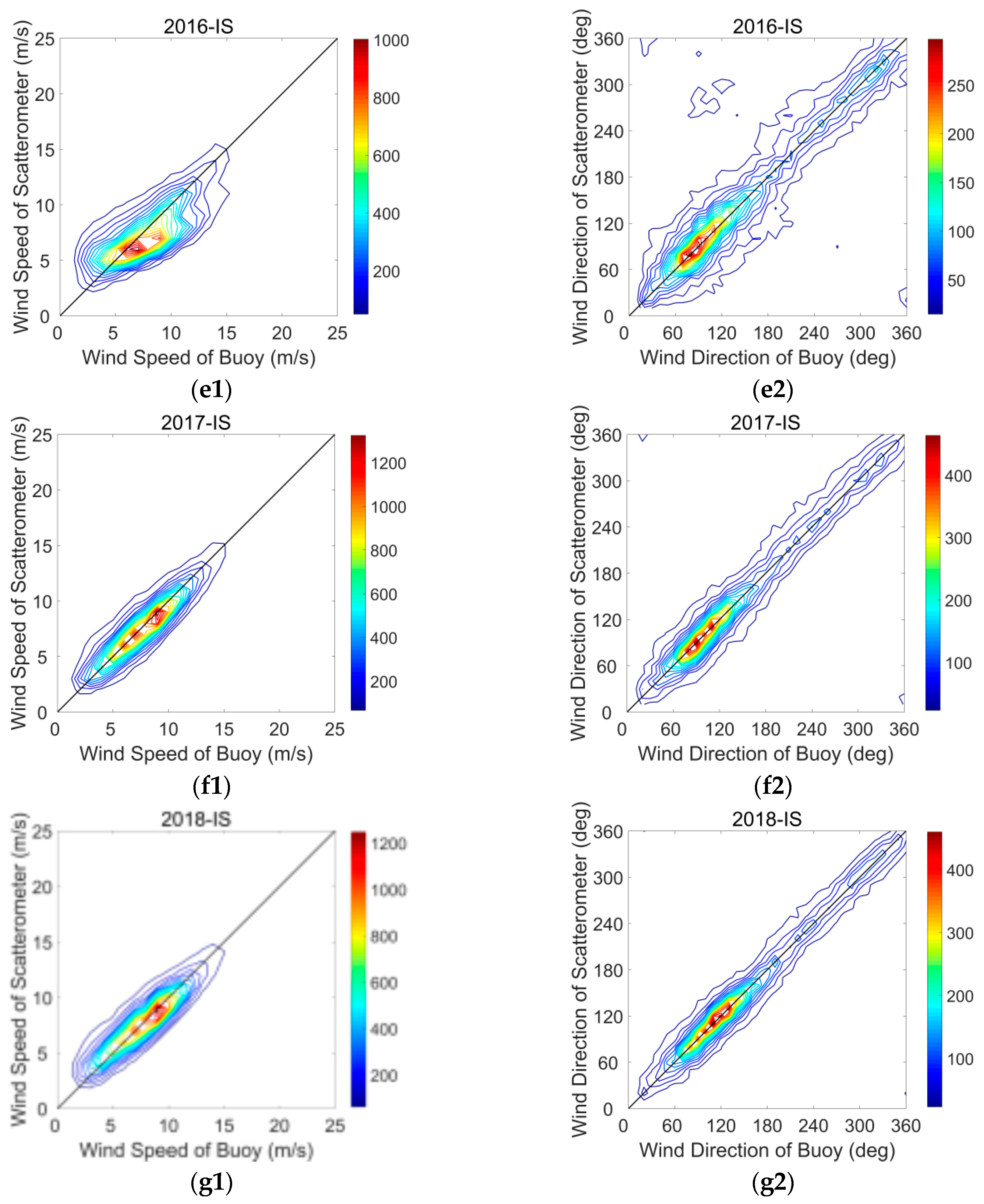
The whole-year HSCAT wind data were compared with the contemporaneous buoy wind data and the wind speed and wind direction collocation contours of histograms are shown in Figure 3 from 2012 to 2018. Figure 3a–g represent the comparisons for each year from 2012 to 2018; number 1 and 2 represent the wind speed and wind direction collocation contours of histograms, respectively.

Figure 3(a1–g1) show that the HSCAT and buoy wind speeds are mainly distributed in the range from 5 to 12 m/s. The consistencies between HSCAT and buoy wind speed descend from 2012 to 2016 but ascend in 2017 and 2018, which shows the HSCAT wind speed product quality variations. The quantified statistics will be analyzed in this subsection later. Wind speed contours in 2013 have a larger dispersion among the contours from 2012 to 2014. The speed contours in 2015 and 2016 deviate from $\mathrm{y}=\mathrm{x}$ and HSCAT wind speeds are higher when speeds are less than 5 m/s but lower when speeds are higher than 10 m/s.

Figure 3(a2–g2) show that the HSCAT and buoy wind direction are mainly distributed in the range from 60° to 150°. Similar with the wind speed, consistencies between the HSCAT and buoy wind direction descend from 2012 to 2016 and then ascend in 2017 and 2018.

The quantitative statistics of the wind vector bias in the collocated winds are given in

Table 2. The statistical parameters of the wind vector bias between HSCAT and buoys.

Year	Speed Bias	Speed RMSE	Direction Bias	Direction RMSE	Collocation Number
2012	−0.03	1.08	0.20	21.75	33,462
2013	0.48	1.42	0.60	22.06	31,276
2014	0.06	1.06	1.23	22.15	27,339
2015	0.26	1.37	0.29	26.37	36,211
2016	−0.41	1.87	1.93	29.50	25,898
2017	−0.14	1.20	2.12	24.50	27,511
2018	0.03	1.17	1.32	22.94	24,997

. Invalid data were removed, the speeds of which are twice as high as the speed’s standard deviation(σ) by using the 2σ quality control method proposed by Lin et al. (2013) [26]. The statistical parameters were calculated using the following equation (here, ‘< >’ represents the statistical average) [9,36]:

$${\mathrm{Bias}}_{spd}=\langle sp{d}_{SCAT}-sp{d}_{BUOY}\rangle ,$$

(2)

$$RMS{E}_{spd}=\sqrt{\langle {\left(sp{d}_{SCAT}-sp{d}_{BUOY}\right)}^2\rangle }.$$

(3)

Wind direction statistical parameters were calculated by using Equations (4)–(7) to ensure the continuity at 0°and 360° [37]:

$$\overline{U}=\langle \sin (di{r}_{SCAT}-di{r}_{BUOY})\rangle ,$$

(4)

$$\overline{V}=\langle \cos \left(di{r}_{SCAT}-di{r}_{BUOY}\right)\rangle ,$$

(5)

$${\mathrm{Bias}}_{dir}=\cot \left(\overline{U}/\overline{V}\right),$$

(6)

$$RMS{E}_{dir}=\cot \sqrt{(\langle si{n}^2\left(di{r}_{SCAT}-di{r}_{BUOY}\right)\rangle /\langle co{s}^2\left(di{r}_{SCAT}-di{r}_{BUOY}\right)\rangle )}.$$

(7)

The statistical parameters in Table 2 explain the quantification of the variation trends shown in Figure 3: HSCAT wind vectors agree well with buoy data in 2012 and 2014 but the average speed bias in 2013 is larger by about 0.4 m/s and the root mean square error (RMSE) is larger by about 0.4 to 0.5 m/s than the statistics in 2012 and 2014. However, in 2015 and 2016, both of the wind speed and wind direction statistics have the greatest offset, in that the speed RMSEs are larger by about 0.2 to 0.4 m/s and the direction RMSEs are larger by 4 to 8° compared to other years. This trend also reflects that the data qualities in 2015 and 2016 and wind speed data quality in 2013 are worse than others.

In terms of yearly variations of the statistical parameters, consistencies between HSCAT and buoy winds are good; wind speed consistencies show a descending trend in 2013 but direction consistencies are similar with 2012. From 2014, wind direction consistencies also descend; both the wind speed and direction show great offsets in 2015 and 2016, but the offsets get smaller in 2017 and 2018 and the data quality in 2018 is similar with 2012.

All in all, the HSCAT wind speed accuracy can satisfy the scatterometer mission requirements (2 m/s) but the wind direction accuracy is a little worse. Besides, the wind data in 2015 and 2016 have the greatest offsets. A strict quality control is needed in the application of these datasets.

3.1.2. The Probability Distribution Functions (PDFs) of Wind Speeds and Directions

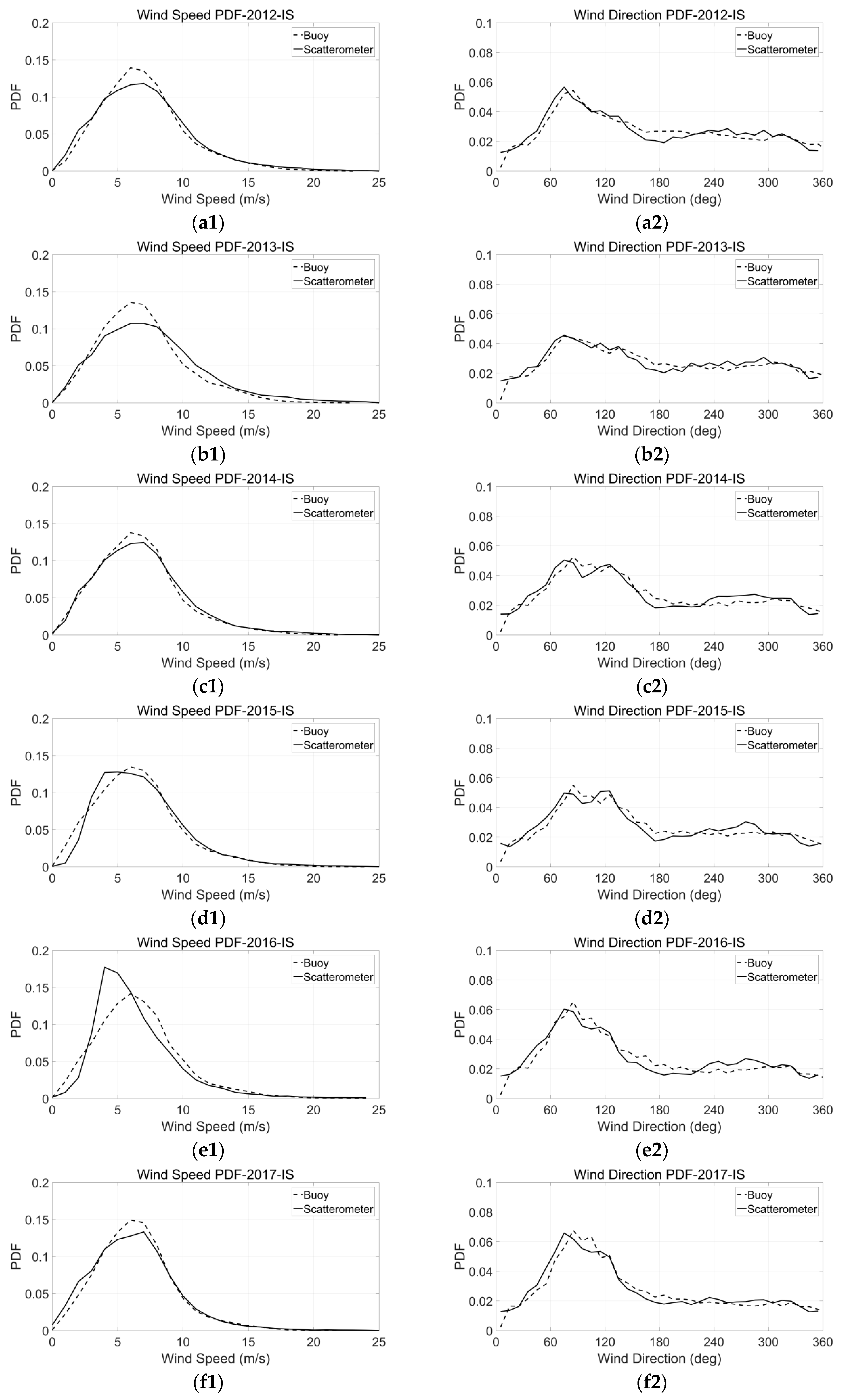
In order to analyze the entire distributions of the collocated data between HSCAT and buoys, we plotted the probability distribution functions (PDFs) of wind speeds and directions for each year. The PDFs are shown in Figure 4 in which a–g represent the PDF curves for each year from 2012 to 2018; number 1 and 2 represent the wind speed and direction PDFs; and the dotted line is the PDF for the buoy data and the solid line for HSCAT PDF.

The HSCAT wind vector PDFs have similar distributions to the buoy PDFs, but they do not agree well in detail. Similar with the results in Section 3.1.1, the HSCAT and buoy wind speeds are mainly distributed in the range from 5 to 12 m/s and the wind directions are mainly distributed in the range from 60° to 150°. Until 2014, the distributions are similar and basically agree well at the peaks. However, the HSCAT PDF curves clearly separate from the buoy curves in 2015 and 2016 but converge in 2017 and 2018.

For wind speed PDFs, the peak values of the buoy data are about 6 to 7 m/s and HSCAT data are distributed at 6 to 8 m/s except in 2016, which is less than 5 m/s. Within the wind speed ranges from 0 to 4 m/s, the numbers of the HSCAT wind speed are slightly higher except in 2015 and 2016; within 4 to 8 m/s, the numbers of the HSCAT wind speed are about 2% lower than the buoys; within 8 to 13 m/s, the numbers of the HSCAT wind speed are generally higher; and when speeds are higher than 13 m/s, the HSCAT speed PDFs are basically consistent with the wind speed PDFs of the buoy data.

For wind direction PDFs, both the HSCAT and buoy peak values are distributed stably about 90 to 110° among seven years. The numbers of the HSCAT wind direction are a little higher when the wind directions are less than 90°; in the range 90–100°, the numbers of the HSCAT direction at the peak values are less than the buoys; the numbers of the HSCAT direction are lower in the range 120–220°, and then become higher in 220 to 330° but become lower again when directions are larger than 330°. From 2014, the HSCAT wind direction PDFs show two little peaks (70–80° and 110–120°) on the main central peak region but disappear in 2018.

In a word, for the annual wind vector PDF distributions, the numbers of HSCAT and buoy wind data are basically the same, but the number distributions vary in different wind speed and wind direction bins.

3.2. The Overall Statistical Analysis of HSCAT Wind Variations from 2012 to 2018

3.2.1. The Trends of Residual Variations of Wind Speed and Wind Direction

The dependencies of the wind speed and direction residual $\left(SCAT-BUOY\right)$ from 2012 to 2018 are shown in Figure 5. In order to study wind speed and direction bias variations in different speed bins, the residuals were calculated in the speed bins of 1 m/s. To avoid a binning effect, we used the average wind speed, (spd_SCAT + spd_BUOY)/2, as the binning wind speed [38]. All collocated data were quality controlled by the 2σ method (Lin et al. 2013). Figure 5a,b represent the wind speed and direction residual distributions; the error bars represent the wind data biases and RMSEs, respectively.

The collocated wind speed data are mostly distributed in the range 3–8 m/s. Average wind speed biases generally increase as wind speeds increase. When wind speeds are in the range 3–11 m/s, wind speed biases are approximately equal to 0. The wind speed RMSEs are less than 2 m/s and have no obvious changes with the increasing speeds. When wind speeds are higher than 10 m/s, wind speed biases are positive; that is, HSCAT wind speeds are higher than buoy wind speeds. Wind speed biases and RMSEs increase with the increasing wind speeds and the average bias and RMSE are about 2 and 3 m/s when the wind speed is 20 m/s. However, the increasing trend of the speed biases and RMSEs can be related with the decreasing collocation numbers. Generally, less data can cause a large offset.

In terms of wind direction, the whole distributions of wind direction bias remain nearly unchanged around zero as wind speeds increase except the bias at 23 m/s (about 120°), which may be caused by the small collocation numbers at the high wind speed region. When wind speeds are less than 5 m/s, the wind direction RMSEs decrease with the increasing speeds and drop from 60° to 20° rapidly. When speeds are higher than 5 m/s, the wind direction RMSEs remain nearly unchanged around 18°.

Both the wind speed and wind direction average biases are near 0 and the RMSEs are less than 2 m/s and 20° at moderate speeds, which means HSCAT wind products basically meet the scatterometer mission requirement. However, larger offsets are found in high speeds, which may be caused by the small numbers of collocated wind data.

3.2.2. HSCAT Wind Field Data Monthly Variations during 2012 to 2018

To further study HSCAT wind field data variations over time, wind speed and direction residual monthly variations are shown in Figure 6. Figure 6a,b represent the wind speed and direction error bars and collocated data histograms during 2012–2018, respectively. The error bars indicate the wind data biases and RMSEs.

As seen from the collocated data histograms, collocation numbers remain stable at around 2000 to 3000 pairs except some months like September in 2015; March, August, and September in 2016; and February in 2017, which is related with the missing records of the HSCAT L2B data.

For wind speed, wind speed data are stable and have just slight offsets compared with buoy data in 2012. The biases are around 0 and the RMSEs are about 1 m/s. In the first half of 2013, the wind speed biases abruptly increase to 1 m/s and the RMSEs also increase to about 1.5 m/s, but the biases then turn to around 0 and the RMSEs decrease to more than 1 m/s in the second half of 2013 to 2015. From 2015 to 2016, the wind speed biases are quite unstable and the RMSEs are obviously larger than other years. The maximum bias is −1.5 m/s and the maximum RMSE is about 2 m/s. From September 2016 to the end of 2017, wind speed biases and RMSEs start decreasing. Those variations show that the HSCAT wind speed products have large offsets and are unstable in 2013, 2015, and 2016, which is in accordance with the results in Section 3.1.1.

Wind direction biases are distributed stably around zero and the RMSEs of the wind direction are about 25°. However, from the second half of 2015, the wind direction biases tend to a 2° positive deviation and RMSEs also increase and increase to 30° in the end of 2016, which are far away from the mission requirement (20°). In 2017, the direction biases and RMSEs both decrease to about 2° and 20° in 2018. The variations of the wind direction are also similar with the statistical parameters mentioned above.

3.2.3. HSCAT Wind Field Data Variations in 24 Hours

The wind speed and direction residual variations during 24 h are shown in Figure 7. These statistics were gathered by the buoy time. Figure 7a,b represent the wind speed and direction error bar graphs and collocated data histograms during 2012–2018, respectively. The error bars indicate the wind data biases and RMSEs.

Figure 7 shows that there is a drop of the collocation numbers at 3 to 4 h later than the HY-2A satellite descending time and have peaks from 2 a.m. to 3 a.m., 11 a.m. to 1 p.m., and 4 p.m. to 6 p.m. This correlation is caused by the sun-synchronous orbit of the HY-2A satellite and the positions of buoys. Wind speed bias variations are stably distributed around 0 in 24 h except in the periods that have less collocation pairs and wind speed RMSEs are generally less than 2 m/s. Wind direction biases are also distributed around 0 and fluctuate within ±2°. However, the RMSEs of the direction are stably distributed around 20 to 30°, which does not satisfy the mission requirement. This suggests that the wind speeds of HSCAT can provide stable speed products in one day with accurate qualities. Unlike the stable daily wind speed residual variations, the wind direction products of HSCAT in one day are not stable or accurate enough to be applied in marine research and these are also similar to the statistical parameters mentioned above.

3.3. The Sea Surface Temperature and Air Temperature Impact on HSCAT Wind Products

Although scatterometers can measure sea surface parameters with all-weather, all-time capabilities, the actual measurements are the sea surface normalized radar cross-section (NRCS), which is affected by both sea and atmospheric conditions. To study the sea and atmospheric parameter impacts on HSCAT wind field retrieval, we classified the collocated data into two groups according to the difference between the sea surface temperature and air temperature measured by buoys: The neutral group (the absolute values of temperature difference are less than or equal to 1 °C) and non-neutral group (the absolute values of temperature difference are higher than 1 °C). After data quality control, we obtained 217,359 pairs of collocations from 2012 to 2018 consisting of 129,604 pairs of the neutral group and 87,755 pairs of the non-neutral group.

3.3.1. The Probability Distribution Functions (PDFs) of Wind Speeds and Directions

We plotted the PDFs of the wind speed and direction for different groups. The PDFs are shown in Figure 8 in which (a) and (b) represent wind speed and direction PDFs; number 1, 2, and 3 represent the neutral group, non-neutral group, and all collocated data PDFs; and the dotted line is the PDF for the buoy data and the solid line for HSCAT PDF, respectively.

As for wind speed, HSCAT PDFs are consistent with the buoy PDFs except the numbers of HSCAT winds are less at the peak values (6–8 m/s). The HSCAT speed PDF is not in good agreement with the buoy PDF at 6 to 8 m/s for the neutral group while the non-neutral group is more consistent. In the neutral group, HSCAT has more collocation numbers when speeds are less than 5 m/s but less numbers than the buoys at 6 to 8 m/s. However, in the non-neutral group, HSCAT has less numbers when speeds are less than 5 m/s. When speeds are higher than 10 m/s, both the neutral and non-neutral group have consistent collocation results.

As for wind direction, the HSCAT and buoy wind directions are mainly distributed in the range 60–120°. Besides, HSCAT has another peak value distributed in the range 240–300°. In the non-neutral group, there is a double peak characteristic of both the HSCAT and buoy PDFs, and the HSCAT PDFs have larger peak values. In the neutral group, HSCAT has more collocation numbers when the directions are less than 70° but less numbers at 90°, where the buoy direction collocation numbers are the maximum.

Generally, the consistency of speed collocation in the neutral group is worse than the non-neutral group but the direction collocation consistency is better in the neutral group. Since the neutral group is the main part of all the collocated data, the overall PDF distribution during 2012 to 2018 is similar to the neutral group.

3.3.2. The Trends of Residual Variations of Wind Speed and Wind Direction

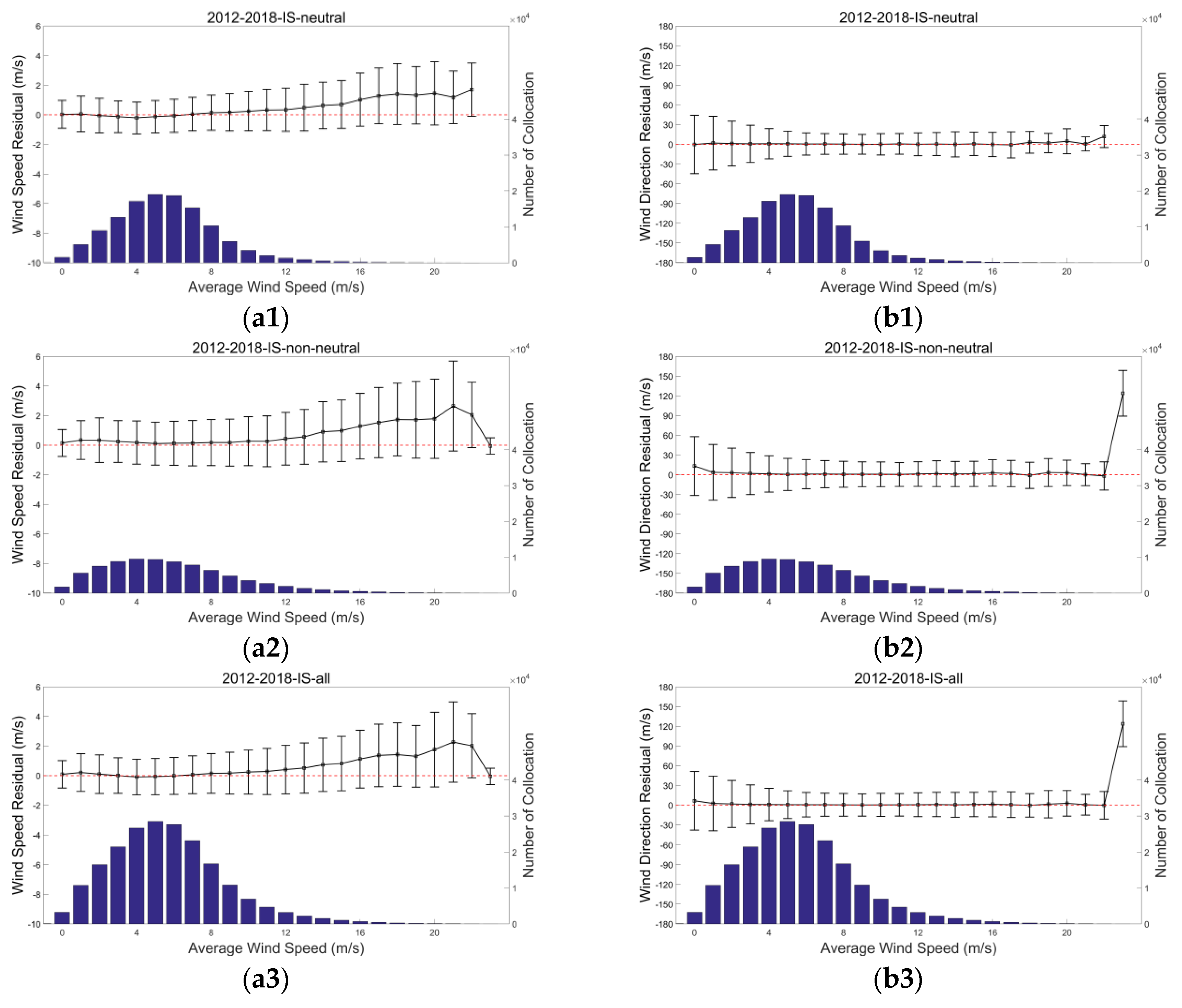
Figure 9 shows the variations of the wind speed and direction residual on the average wind speed from 2012 to 2018 under different stratification conditions. We also used the average wind speed as the binning wind speed with 1-m/s intervals to avoid the binning effect. In Figure 9, a and b represent the wind speed and direction residual distributions; 1, 2, and 3 represent the neutral group, non-neutral group, and all collocation data residual distributions; and the error bars represent the wind data biases and RMSEs, respectively.

For both the neutral and non-neutral group, the average speed biases are distributed around 0 in 0 to 12 m/s and the biases increase with increasing speeds. The speed RMSEs of the neutral group are about 1 m/s, but the RMSEs of the non-neutral group are larger (about 2 m/s). When the wind speed is higher than 12 m/s, the average speed biases start increasing in both groups. The speed biases of the neutral group are about 1.5 m/s and the RMSEs increase to about 1.5 m/s in the range 16–20 m/s. Additionally, in this range, the non-neutral group’s average wind speed biases and RMSEs are larger. When the speed equals 20 m/s, the bias and RMSE increase to about 2 m/s and 2.5 to 3 m/s, respectively.

For wind direction, the biases remain nearly unchanged around zero. In 0 to 5 m/s, both RMSEs of the neutral and non-neutral groups decrease from 45° to 20°. When the wind speed is higher than 5 m/s, the RMSEs of the neutral group are about 25° while the RMSEs of the non-neutral group are about 30°. Both the wind speed and direction biases of the non-neutral group have large changes at 23 m/s, which may be connected with the small collocation numbers at 23 m/s.

3.3.3. The Statistical Parameters of Collocated Data

For further study of the winds’ residual variations under neutral and non-neutral conditions, the quantitative statistics of the wind vector difference between HSCAT and buoys are given in

Table 3. The statistical parameters of the wind vector bias between HSCAT and buoys under different stratification conditions.

Year	Wind Speed (m/s)				Wind Direction (°)				Collocation Number
	Bias-Neutral	Bias-Non-Neutral	RMSE-Neutral	BMSE-Non-Neutral	Bias-Neutral	Bias-Non-Neutral	RMSE-Neutral	BMSE-Non-Neutral	Neutral	Non-Neutral
2012	−0.12	0.14	0.95	1.31	0.15	0.30	19.89	24.47	20,596	13,908
2013	0.37	0.65	1.24	1.66	0.55	0.75	20.28	24.26	17,593	13,691
2014	−0.03	0.19	0.93	1.23	0.93	1.61	19.99	24.81	15,427	11,917
2015	0.18	0.42	1.17	1.67	0.18	0.44	23.84	29.95	21,446	14,793
2016	−0.52	−0.23	1.85	1.92	1.77	2.21	28.97	30.36	15,913	9990
2017	−0.23	0.07	1.05	1.48	1.34	3.61	22.44	27.96	17,474	10,047
2018	−0.03	0.19	1.01	1.48	1.08	1.84	19.99	27.64	15,995	9038
ALL	−0.02	0.25	1.15	1.53	0.82	1.35	24.58	31.68	123,819	83,179

.

After data quality control, generally, the number of the neutral group is 1.3 to 1.8 times the non-neutral group number. Those statistical parameters also validate the results in Section 3.3.1 and Section 3.3.2 that the winds’ average biases and RMSEs of the neutral group are less than the non-neutral group; both groups of the HSCAT wind speed can meet the mission requirement but the RMSEs of the wind direction are much higher than 20°, especially in the non-neutral group, which can reach 30°.

For wind speed, the biases of the non-neutral group are about 0.2 m/s higher than the neutral group except in 2016, which is about 0.4 m/s higher, but they all meet the mission requirement. In 2013, 2015, and 2016, both the neutral and non-neutral groups’ offsets are much larger than other years. Except in 2015, the average wind speed bias of the neutral group is similar to other years but much larger under non-neutral conditions. Those large offsets decrease in 2017 and 2018.

For wind direction, the average biases are quite small from 2012 to 2015. However, after 2015, the average biases are more than 1° and the RMSEs are quite large whether under neutral conditions or non-neutral conditions, although the RMSEs of the neutral group are less 4 to 6° compared to the non-neutral group. From 2012 to 2014, the direction RMSEs of the neutral group are less than 20° and start increasing from 2015. In 2016, both the neutral and non-neutral groups’ RMSEs increase to 30° and then decrease in 2017, but wind direction RMSEs under non-neutral conditions are still about 7° higher than the mission requirement.

HSCAT wind products can meet the mission requirement under neutral conditions. Under non-neutral conditions, wind speeds can also satisfy the requirement while wind direction offsets are large. In terms of the variations of statistics, although wind speed biases in 2013, 2015, and 2016 are larger than the other years, the data can still meet the requirement. Wind direction biases and RMSEs increase from 2015 and RMSEs of the non-neutral group in 2016 can get to 30°. Under non-neutral conditions, variations of the wind direction are larger than the wind speed, which shows that HSCAT wind direction retrieval is more susceptible than the wind speed to sea and atmospheric parameters. Besides, wind speed and direction offsets are large whether for the neutral group or non-neutral group in 2016 and the offset differences are less than other years, which illustrates the worst quality for the 2016 product in an indirect way. After 2015, HSCAT wind products need strict quality control, especially the wind direction products when HSCAT wind data are used in marine studies.

3.4. The Rain Impact on HSCAT Wind Products

As mentioned above, the sea surface wind field is retrieved from scatterometer NRCS, which is affected by sea surface roughness. At different rainfall rates, the changes of the sea surface roughness are complicated. Besides, the rain drop size and density also have an impact on the return signal scattering. Therefore, dealing with rain contaminated data is one of the difficulties in scatterometer wind retrieval. It is especially important for scatterometer data usage under rainy conditions to study HSCAT wind field variations at different rainfall rates [20].

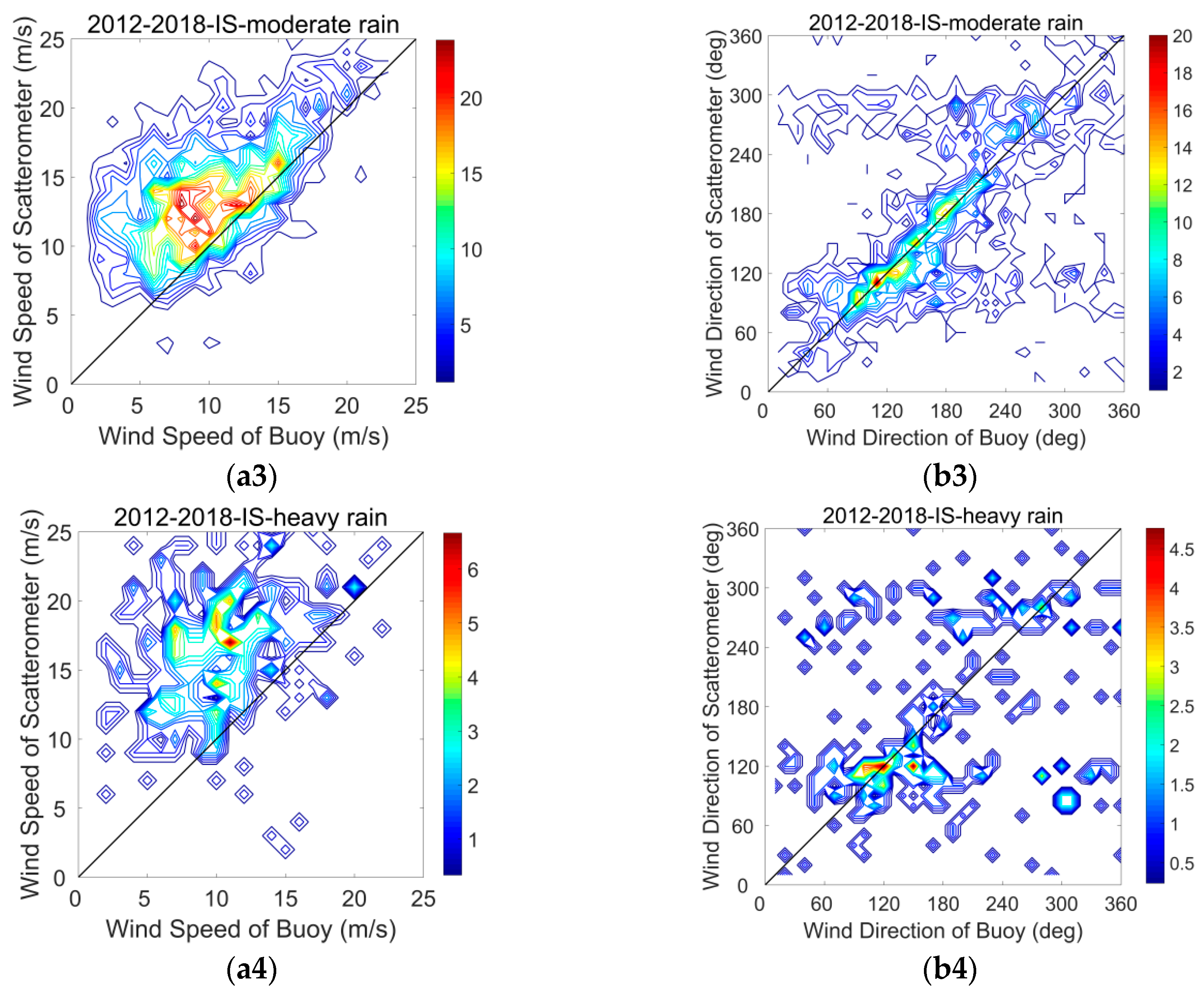
We collocated the HSCAT and buoy collocation dataset with SSMIS data within 1 h. We divided rain collocation data into four groups according to different rainfall rates: Rain free (rainfall rate equals to 0 mm/h), light rain (rainfall rate is from 0 to 3 mm/h), moderate rain (rainfall rate is from 3 to 8 mm/h), and heavy rain (rainfall rate is higher than 8 mm/h). To avoid the extra offsets caused by small numbers of rain sample data, we studied all the rain collocated data from 2012 to 2018.

3.4.1. The Distribution of Collocated Data and Statistical Parameters

We compared HSCAT wind data with buoy wind data, and the wind speed and wind direction collocation contours of histograms are shown in Figure 10. Figure 10a,b represent the wind speed and direction collocation contours of histograms; number 1 to 4 represent collocation contours of histograms of the rain free group, light rain group, moderate rain group, and heavy rain group, respectively.

It is evident that the collocation numbers decrease with an increasing rainfall rate and both the wind speed and direction collocation contours appear as losing trends. As for wind speed, the speed contours move to the top of the figure with the increasing rainfall rate, which means HSCAT-retrieved wind speeds are increasingly overestimated. HSCAT wind speeds are almost twice the buoy speeds and have large deviation in heavy rain. As for wind direction, HSCAT wind direction numbers increase in the range 60–120° and 240–300°, which means that the HSCAT wind directions tend to be perpendicular to the buoy directions. The two-peak characteristic is evidently shown in Figure 10, which increases the wind direction estimation errors.

We also calculated the statistics of the wind vector biases in different rainfall rates, which are given in

Table 4. The statistical parameters of the wind vector bias between HSCAT and buoys in different rainfall rates.

Rainfall Rate	Speed Bias	Speed RMSE	Direction Bias	Direction RMSE	Collocation Number
Rain free	0.05	1.73	1.00	24.10	121,080
0–3 mm/h	1.14	2.86	1.36	29.09	11,021
3–8 mm/h	3.73	5.38	−0.04	35.57	1683
>8 mm/h	6.16	7.94	3.42	38.44	291

.

The statistical parameters also illustrate the decreasing collocation numbers and increase of the wind speed and direction offsets with an increasing rainfall rate. The average biases of the wind speed increased and RMSEs also multiplied with the increasing rainfall rate, i.e., the higher the rainfall rate, the worse the HSCAT-retrieved wind speed product. Besides, the positive biases of the wind speed also increase, which reflects that the overestimation of the retrieved speeds is also increasing with the rainfall rate. In the rain-free group, the wind speed and direction can satisfy the mission requirement. In the light rain group, the wind speed RMSEs are over 2 m/s, which reflects that the HSCAT-retrieved speed data need quality control even under light rain conditions. Similar to the wind speed, the wind direction data quality greatly decreases with the increasing rainfall rate. The wind direction RMSEs are almost 40° under heavy rain conditions, i.e., twice the mission requirement. The wind direction is also a little larger than the requirement even in the rain-free group.

Therefore, HSCAT can basically satisfy the marine study requirement under rain-free conditions, although HSCAT wind directions have larger offsets. In rainfall conditions, both the speed and direction offsets are larger than the requirement. When the rainfall rate is higher than 3 mm/h, we do not recommend the use of HSCAT wind products due to their large deviations. It is also a key problem to be resolved in order to improve the accuracy of HSCAT wind retrieval in rainfall conditions.

3.4.2. The Probability Distribution Functions (PDFs) of Wind Speeds and Directions

We plotted the PDFs of wind speeds and directions in different rainfall rates from 2012 to 2018 as shown in Figure 11 with a speed of 1 m/s and a 10° direction interval. (a) and (b) represent the wind speed and direction PDFs; number 1 to 4 represent the rain-free group, light rain group, moderate rain group, and heavy rain group PDFs; and the dotted line is the PDF for the buoy data and the solid line is for HSCAT PDF, respectively.

The wind speed and direction PDFs reconfirm the results in Section 3.4.1.

For wind speed, the distributions of the buoy speed are mainly distributed in 6 to 8 m/s and are nearly unchanged with the increasing rainfall rate. Therefore, the buoy speed PDFs’ fluctuation can be regarded as changes of the ocean environment and the decreasing of collocations with the increasing rainfall rate. However, the entire distribution of the buoy speed is stable so that the buoy speed can be a reliable evaluation standard. However, the peaks of the HSCAT wind speed PDFs move from 5 to 6 m/s under the rain free condition to 16 to 18 m/s under the heavy rain condition. The overestimation of the HSCAT speed increases as the rainfall rate increases, and the HSCAT speeds of the heavy rain group are almost twice the buoy speeds.

For wind direction, the rain free buoy wind directions are mainly distributed in the range 60–120° and then slightly move to 180° with an increasing rainfall rate. However, the movement is quite small so the buoy direction can be seen as a relatively stable evaluation standard. Similar with the results in Section 3.4.1, under the rain-free condition, the HSCAT and buoy direction PDFs are consistent well. However, with the rainfall rate increasing, the HSCAT wind directions have two peaks in the ranges 60–120° and 240–300° with growing peak values, and the extent of the two PDFs’ separation increases. It illustrates that HSCAT-retrieved wind directions tend to be perpendicular to the true directions with an increasing rainfall rate, which causes large wind direction offsets under rainy conditions.

4. Conclusions

The stabilities of the HY-2A scatterometer in different times, atmospheric stratification conditions, and rainfall rates were analyzed by comparing HSCAT L2B wind products with buoy wind measurements from 2012 to 2018. In the study, HSCAT and buoy data were selected within the range 0.1–25 m/s and collocated within $25/\sqrt{2}$ km (about 17.7 km) and 30 min. After data quality control, yearly matching data were 34,462, 31,276, 27,339, 36,211, 25,898, 27,511, and 24,997 pairs from 2012 to 2018. According to the collocated data, wind speed biases and RMSEs between HSCAT and buoy measurements were about 0.1 to 0.2 m/s and 1.2 m/s while biases and RMSEs of the wind direction were 1° and 27°, respectively. These suggest that HSCAT wind direction accuracy is slightly worse than the scatterometer mission requirement (20°). The yearly PDF curves also supported these results. In 2015 and 2016, the HSCAT PDFs and buoy PDFs showed clear separation and then tended to agree with each other in 2017. From 2017, HSCAT winds and buoy winds had similar distributions and the offsets tended to decrease.

For wind speed and direction bias variations in different speed bins, the collocated data were mostly distributed in the speed range 6–8 m/s. The minimums of the wind speed bias and RMSE were distributed around 3 to 11 m/s while the minimums of the wind direction biases and RMSEs appeared when speeds are higher than 5 m/s. When speeds are higher than 10 m/s, the average speed biases and RMSEs were increased with increasing binning speeds. The wind direction offsets were barely changed, except the RMSEs of the wind direction increased slightly when speeds were higher than 16 m/s.

According to the HSCAT wind field data variations over time, wind speed and direction average biases were distributed around 0. Wind speed RMSEs were about 2 m/s and wind direction RMSEs were about 20 to 30°. HSCAT wind speed biases were a little larger in 2013, and HSCAT wind products were the most unstable in 2015 and 2016, which had the largest offsets and variations among the seven years.

To study the atmospheric stratification impacts on HSCAT wind products, we classified the collocated data into a neutral group (the absolute values of temperature difference are less than 1 °C) and non-neutral group (the absolute values of temperature difference are higher than 1 °C) according to the differences between the sea surface temperature and air temperature and then analyzed the wind field error features in the different groups. The wind PDFs and error characteristic variations with the wind speeds illustrated that the quality of HSCAT-retrieved wind products are better in neutral conditions. Wind direction has more of an influence from marine and atmosphere environmental parameters and owns large changes in the non-neutral condition. From the yearly statistical parameters of the collocated data, the HSCAT wind product qualities declined from 2015 but were improved from 2017. In 2016, the offset differences between the neutral and non-neutral group were less than other years, which reflects the worst quality in an indirect way and the data in 2016 need to be treated very carefully in applications.

We also studied the rain impacts on HSCAT wind products. We divided rain-collocated data into a rain-free group (0 mm/h), light rain group (0–3 mm/h), moderate rain group (3–8 mm/h), and heavy rain group (>8 mm/h) according to the rainfall rate. From the wind PDFs and collocated contours, we found that the accuracy of the HSCAT-retrieved wind field decreases as the rainfall rate increases: HSCAT-retrieved wind speeds and the RMSEs of collocated speeds increased with an increasing rainfall rate; HSCAT-retrieved wind directions tended to concentrate on the 60–120° and 240–300° ranges, which means HSCAT-retrieved wind directions tend to be perpendicular to the true directions. These results may provide references for the correction of scatterometer rain-contaminated data.

Overall, HSCAT L2B wind products are less accurate and less stable than the mission requirement especially for wind direction products during 2012 to 2018. The qualities of HSCAT operational wind products declined from 2012 to 2016 but were improved from 2017. HSCAT wind products should be treated carefully, especially in 2015 and 2016, or adopt other ways to improve data qualities when HSCAT wind data are used in marine studies.

Long-term evaluation for HSCAT wind products was analyzed in this study, and we also studied the error characteristics in different times, atmospheric stratification conditions, and rainfall rates primarily. However, only a little collocated data was distributed in the high wind speed region due to the lack of high speed data from buoys. The reasons for quality improvement from 2017 were not discussed here. Comparing HSCAT wind data with other satellite scatterometer data, studying the environmental parameter impacts on scatterometers working in different bands, finding improvement methods for HSCAT winds, and other related studies need to be investigated in the future.

References

1. Liu, L. An Introduction to Satellite Oceanic Remote Sensing; Wuhan University Press: Wuhan, China, 2005; pp. 245–264. [Google Scholar]
2. Zhixiong, W. The Improvement of HY2-SCAT Wind Retrieval Algorithm Based on MSS and 2DVAR Method. Master’s Thesis, Ocean University of China, Qindao, China, 2014. [Google Scholar]
3. Wang, X.; Yang, B. Abroad satellite microwave scatterometer application and the trends. Erospace China 2006, 26–29. [Google Scholar]
4. Yang, J.; Zhang, J. Evaluation of ISS-RapidScat Wind Vectors Using Buoys and ASCAT Data. Remote Sens. 2018, 10, 648. [Google Scholar] [CrossRef] [Green Version]
5. Crapolicchio, R.; Lecomte, P. The ERS-2 scatterometer mission: Events and long-loop instrument and data performances assessment. In Proceedings of the 2004 ENVISAT & ERS Symposium, Salzburg, Austria, 6–10 September 2004; pp. 6–10. [Google Scholar]
6. Spencer, M.W. A Methodology for the Design of Spaceborne Pencil-Beam Scatterometer Systems. Ph.D. Thesis, Brigham YoungUniversity, Provo, UT, USA, 2001. [Google Scholar]
7. Gelsthorpe, R.; Schied, E.; Wilson, J. ASCAT-Metop‘s advanced scatterometer. ESA Bull. 2000, 102, 19–27. [Google Scholar]
8. Graf, J.; Sasaki, C.; Winn, C.; Liu, W.T.; Tsai, W.; Freilich, M.; Long, D. NASA Scatterometer Experiment1. Acta Astronaut. 1998, 43, 397–407. [Google Scholar] [CrossRef]
9. Department of Space, Indian Space Research Organisation. Available online: https://www.isro.gov.in/Spacecraft/oceansat-2 (accessed on 20 September 2019).
10. National Satellite Ocean Application Service. Available online: http://www.nsoas.org.cn/news/content/2018-10/25/44_531.html (accessed on 20 September 2019).
11. Masuko, H.; Arai, K.; Ebuchi, N.; Konda, M.; Kubota, M.; Kutsuwada, K.; Manabe, T.; Mukaida, A.; Nakazawa, T.; Nomura, A. Evaluation of vector winds observed by NSCAT in the seas around Japan. J. Oceanogr. 2000, 56, 495–505. [Google Scholar] [CrossRef]
12. Ebuchi, N.; Graber, H.C.; Caruso, M.J. Evaluation of wind vectors observed by QuikSCAT/SeaWinds using ocean buoy data. J. Atmos. Ocean. Technol. 2002, 19, 2049–2062. [Google Scholar] [CrossRef]
13. Pickett, M.H.; Tang, W.; Rosenfeld, L.K.; Wash, C.H. QuikSCAT satellite comparisons with nearshore buoy wind data off the US west coast. J. Atmos. Ocean. Technol. 2003, 20, 1869–1879. [Google Scholar] [CrossRef] [Green Version]
14. Tang, W.; Liu, W.T.; Stiles, B.W. Evaluation of high-resolution ocean surface vector winds measured by QuikSCAT scatterometer in coastal regions. IEEE Trans. Geosci. Remote Sens. 2004, 42, 1762–1769. [Google Scholar] [CrossRef]
15. Ebuchi, N. Intercomparison of Wind speeds observed by AMSR and SeaWinds on ADEOS-II. In Proceedings of the 2005 IEEE International Geoscience and Remote Sensing Symposium (IGARSS’05), Seoul, Korea, 29 July 2005; pp. 3314–3317. [Google Scholar]
16. Satheesan, K.; Sarkar, A.; Parekh, A.; Kumar, M.R.R.; Kuroda, Y. Comparison of wind data from QuikSCAT and buoys in the Indian Ocean. Int. J. Remote Sens. 2007, 28, 2375–2382. [Google Scholar] [CrossRef]
17. Yang, X.; Li, X.; Pichel, W.G.; Li, Z. Comparison of ocean surface winds from ENVISAT ASAR, MetOp ASCAT scatterometer, buoy measurements, and NOGAPS model. IEEE Trans. Geosci. Remote Sens. 2011, 49, 4743–4750. [Google Scholar] [CrossRef]
18. Sudha, A.K.; Prasada Rao, C.V.K. Comparison of Oceansat-2 scatterometer winds with buoy observations over the Indian Ocean and the Pacific Ocean. Remote Sens. Lett. 2013, 4, 171–179. [Google Scholar] [CrossRef]
19. Wang, H.; Zhu, J.; Lin, M.; Huang, X.; Zhao, Y.; Chen, C.; Zhang, Y.; Peng, H. First six months quality assessment of HY-2A SCAT wind products using in situ measurements. Acta Oceanol. Sin. 2013, 32, 27–33. [Google Scholar] [CrossRef]
20. Xing, J.; Shi, J.; Lei, Y.; Huang, X.-Y.; Liu, Z. Evaluation of HY-2A Scatterometer Wind Vectors Using Data from Buoys, ERA-Interim and ASCAT during 2012–2014. Remote Sens. 2016, 8, 390. [Google Scholar] [CrossRef] [Green Version]
21. Bhaskar, T.V.S.U.; Jayaram, C.; Bansal, S.; Mohan, K.K.; Swain, D. Generation and Validation of two Day Composite Wind Fields from Oceansat-2 Scatterometer. J. Indian Soc. Remote Sens. 2016, 45, 113–122. [Google Scholar] [CrossRef]
22. Lindsley, R.D.; Blodgett, J.R.; Long, D.G. Analysis and validation of high-resolution wind from ASCAT. IEEE Trans. Geosci. Remote Sens. 2016, 54, 5699–5711. [Google Scholar] [CrossRef]
23. Verhoef, A.; Vogelzang, J.; Verspeek, J.; Stoffelen, A. Long-Term Scatterometer Wind Climate Data Records. IEEE J. Sel. Top. Appl. Earth Obs. Remote Sens. 2017, 10, 2186–2194. [Google Scholar] [CrossRef]
24. Wentz, F.J.; Ricciardulli, L.; Rodriguez, E.; Stiles, B.W.; Bourassa, M.A.; Long, D.G.; Hoffman, R.N.; Stoffelen, A.; Verhoef, A.; O’Neill, L.W. Evaluating and extending the ocean wind climate data record. IEEE J. Sel. Top. Appl. Earth Obs. Remote Sens. 2017, 10, 2165–2185. [Google Scholar] [CrossRef] [Green Version]
25. Hutchings, N.; Long, D.G. Improved Ultrahigh-Resolution Wind Retrieval for RapidScat. IEEE Trans. Geosci. Remote Sens. 2018, 57, 3370–3379. [Google Scholar] [CrossRef]
26. Lin, M.; Zou, J.; Xie, X.; Zhang, Y. HY-2A Microwave Scatterometer Wind Retrieval Algorithm. Eng. Sci. 2013, 15, 68–74. [Google Scholar]
27. HY-2A Microwave Scatterometer Data Format User’s Guide, National Satellite Ocean Application Service. May 2012. Available online: http://ftp2.nsoas.org.cn/Data_Format_User’s_Guide/HY-2A Microwave Scatterometer Data Format User’s Guide.pdf (accessed on 20 September 2019).
28. Liu, W.T.; Katsaros, K.B.; Businger, J.A. Bulk parameterization of air-sea exchanges of heat and water vapor including the molecular constraints at the interface. J. Atmos. Sci. 1979, 36, 1722–1735. [Google Scholar] [CrossRef] [Green Version]
29. Liu, W.T.; Tang, W.Q. Equivalent Neutral Wind; Jet Propulsion Laboratory Publication 96-17; 1996. Available online: https://ntrs.nasa.gov/archive/nasa/casi.ntrs.nasa.gov/19970010322.pdf (accessed on 4 April 2019).
30. de Kloe, J.; Stoffelen, A.; Verhoef, A. Improved use of scatterometer measurements by using stress-equivalent reference winds. IEEE J. Sel. Top. Appl. Earth Obs. Remote Sens. 2017, 10, 2340–2347. [Google Scholar] [CrossRef]
31. Remote Sensing Systems. Available online: http://www.remss.com/missions/ssmi (accessed on 20 September 2019).
32. Remote Sensing Systems. Available online: http://www.remss.com/support/crossing-times/ (accessed on 20 September 2019).
33. Portabella, M.; Stoffelen, A. Qual. Control. Wind Retrieval for Sea Winds; Ministerie van Verkeer en Waterstaat, Koninklijk Nederlands Meteorologisch: De bilt, The Nederlands, 2002; pp. 7–9.
34. Stiles, B.W.; Pollard, B.D.; Dunbar, R.S. Direction interval retrieval with thresholded nudging: A method for improving the accuracy of QuikSCAT winds. IEEE Trans. Geosci. Remote Sens. 2002, 40, 79–89. [Google Scholar] [CrossRef] [Green Version]
35. Portabella, M.; Stoffelen, A. A probabilistic approach for SeaWinds data assimilation. Q. J. R. Meteorol. Soc. 2004, 130, 127–152. [Google Scholar] [CrossRef] [Green Version]
36. QuikSCAT Scatterometer Mean Wind Field Products User Manual, The CERSAT (Centre ERS d’Archivage et de Traitement)/Laboratory of Oceanography From Space is part of IFREMER (French Research Institute for Exploitation of the Sea), Version 1.0. May 2002. Available online: http://apdrc.soest.hawaii.edu/doc/qscat_mwf.pdf (accessed on 14 September 2018).
37. Qiu, C.; Li, D. The Calculation Algorithms for Average Wind Direction and Their Comparison. Plateau Meteorol. 1997, 94–98. [Google Scholar]
38. Stoffelen, A. Toward the true near-surface wind speed: Error modeling and calibration using triple collocation. J. Geophys. Res. Ocean. 1998, 103, 7755–7766. [Google Scholar] [CrossRef]
Figure 1. The location of buoys used in this study. The black points are offshore stations (more than 50 km away from the coast), and the red triangles are nearshore stations (within 50 km from the coast).
Remotesensing 11 02968 g001
Figure 2. HSCAT cross-track wind cells.
Remotesensing 11 02968 g002
Figure 3. Contours of histograms of comparisons between HSCAT and buoy wind data. (a)–(g) represent the comparisons for each year from 2012 to 2018; number 1 and 2 represent the wind speed collocation contours of the histograms and the wind direction collocation contours of the histograms, respectively.
Remotesensing 11 02968 g003aRemotesensing 11 02968 g003b
Figure 4. Probability distribution functions (PDFs) between HSCAT and buoys during 2012–2018. (a)–(g) represent the PDF curves for each year from 2012–2018; number 1 and 2 represent the wind speed and direction PDFs; the dotted line is the PDF for the buoy data and the solid line for HSCAT PDF.
Remotesensing 11 02968 g004aRemotesensing 11 02968 g004b
Figure 5. Dependencies of the wind speed and direction residual ( S C A T B U O Y ) on the average wind speed. Calculation bins of the average wind speed is 1 m/s. (a,b) represent the wind speed and direction residual distribution; the error bars represent the wind data biases and root mean square errors (RMSEs).
Remotesensing 11 02968 g005
Figure 6. Monthly variations of the wind speed and wind direction residual. (a) shows the variations of the wind speed residual (above) and the collocated data histograms (below) during 2012–2018; (b) represents the variations of the wind direction residual (above) and the collocated data histograms (below) during 2012–2018.
Remotesensing 11 02968 g006
Figure 7. Daily variations of the wind speed and wind direction residual. (a,b) represent wind speed and direction error bars and collocated data histograms, respectively.
Remotesensing 11 02968 g007
Figure 8. Probability distribution functions (PDFs) between HSCAT and buoys under different stratification conditions. (a,b) represent the wind speed and direction PDFs; the number 1, 2, and 3 represent the neutral group, non-neutral group, and all collocation data PDFs; the dotted line is the PDF for the buoy data and the solid line is for HSCAT PDF, respectively.
Remotesensing 11 02968 g008
Figure 9. Dependencies of the wind speed and direction residual ( S C A T B U O Y ) on the average wind speed under different stratification conditions. Calculation bins of the average wind speed are 1 m/s. (a,b) represent the wind speed and direction residual distribution; 1, 2, and 3 represent the neutral group, non-neutral group, and all collocation data residual distributions; the error bars represent the wind data biases and RMSEs, respectively.
Remotesensing 11 02968 g009
Figure 10. Contours of histograms between HSCAT and buoy wind data in different rainfall rate. (a,b) represent the wind speed and direction collocation contours of histograms; number 1 to 4 represent the collocation contours of histograms of the rain free group, light rain group, moderate rain group, and heavy rain group, respectively.
Remotesensing 11 02968 g010aRemotesensing 11 02968 g010b
Figure 11. Probability distribution functions (PDFs) between HSCAT and buoys under different rainfall rates. (a,b) represent wind speed and direction PDFs; number 1 to 4 represent the rain-free group, light rain group, moderate rain group, and heavy rain group PDFs; dotted line is the PDF for buoy data and solid line for HSCAT PDF, respectively.
Remotesensing 11 02968 g011aRemotesensing 11 02968 g011b