Active Semi-Supervised Random Forest for Hyperspectral Image Classification

Abstract

Random forest (RF) has obtained great success in hyperspectral image (HSI) classification. However, RF cannot leverage its full potential in the case of limited labeled samples. To address this issue, we propose a unified framework that embeds active learning (AL) and semi-supervised learning (SSL) into RF (ASSRF). Our aim is to utilize AL and SSL simultaneously to improve the performance of RF. The objective of the proposed method is to use a small number of manually labeled samples to train classifiers with relative high classification accuracy. To achieve this goal, a new query function is designed to query the most informative samples for manual labeling, and a new pseudolabeling strategy is introduced to select some samples for pseudolabeling. Compared with other AL- and SSL-based methods, the proposed method has several advantages. First, ASSRF utilizes the spatial information to construct a query function for AL, which can select more informative samples. Second, in addition to providing more labeled samples for SSL, the proposed pseudolabeling method avoids bias caused by AL-labeled samples. Finally, the proposed model retains the advantages of RF. To demonstrate the effectiveness of ASSRF, we conducted experiments on three real hyperspectral data sets. The experimental results have shown that our proposed method outperforms other state-of-the-art methods.

1. Introduction

Hyperspectral remote sensing can obtain a great deal of information about an object via hundreds of narrow, continuous spectral bands. Hyperspectral imaging techniques have been widely used in many applications, such as landmine detection [1], agricultural monitoring [2], land cover classification [3], and target detection [4]. Many of these applications are based on hyperspectral image (HSI) classification at the pixel level. In the past few years, various supervised classification methods, e.g., support vector machines (SVMs) [5,6], neural networks [7,8], and random forests (RFs) [9,10,11] have been successfully used for HSI classification. However, supervised methods often require many informative samples with labels to train high-performing classifiers. In other words, the quality and quantity of the training data are very important for training good classifiers [12]. However, labeling samples manually requires significant labor, hence, we need a classifier that can perform well with only a few labeled samples. Semi-supervised learning (SSL) [13] and active learning (AL) [14,15] provide promising solutions to improve generalization performance in the case of limited samples. In this paper, we consider combining AL and SSL into random forest for HSI classification.

Random forest, proposed by Breiman [16], is one of the most important machine learning methods. Compared with other machine learning methods, RF has the following advantages [9,10,11,17,18,19,20,21,22,23,24]. First, RF is suitable for high-dimensional data, which can alleviate the influence of curse of dimensionality [20]. Second, RF is very fast because it is implemented in parallel [9]. Third, RF is effective to handle data with imbalanced class labels or missing values [21]. Fourth, RF is not easy to fall into overfitting compared with the Boosting method [18]. Moreover, RF measures the importance of variables automatically [25]. Finally, RF can obtain a higher classification accuracy compared to other well-known classifiers such as SVM [5,6] and maximum likelihood (ML) [17,23], with fewer parameters.

Active learning is a kind of iterative method that queries the most informative samples for manual labeling at each iteration [14]. Initially, the data set consists of two parts: a small number of labeled samples and a large number of unlabeled samples. At each iteration, a query function is adopted to investigate the unlabeled samples and select the most informative samples for manual labeling. After multiple iterations, the performance of the classifier improves along with the increase in the number of manually labeled samples. The query function plays an important role in determining the samples selected for manual labeling, which directly affects the classification performance [15].

Semi-supervised learning, another way to tackle the issue of limited samples, trains a classifier with the labeled and unlabeled samples together, which does not require human labeling. For example, co-training [26,27] and self-training [28,29] iteratively assign pseudolabels to unlabeled samples during the training process. Graph-based methods [30,31] propagate labels from labeled samples to unlabeled samples through the graph. Other SSL methods [32,33] use the unlabeled samples to regularize the training process without pseudolabels. Recently, hubness-aware classifier [34,35] was introduced into SSL. For example, Buza [35] first introduced a semi-supervised hubness-aware classifier for the classification of gene expression data. In addition, clustering technique was widely used for SSL. Marussy and Buza [36] proposed a semi-supervised time-series classifier based on constrained hierarchical clustering and dynamic time warping. Peikari et al. [37] investigated the possibility of using clustering analysis to identify the underlying structure of the data space for SSL.

AL and SSL involve different mechanisms but have the same goal of using limited labeled samples to achieve good generalization performance. Hence, combining AL and SSL is reasonable, and several related approaches have been proposed for HSI classification in recent years. For example, Li et al. [38] adopted multinomial logistic regression with AL to segment HSIs in a semi-supervised manner. Munoz-Mari et al. [39] utilized AL to improve the classification confidence of a hierarchical model by having it select the most informative samples. AL has also been adapted to a co-training framework in which the algorithm automatically selects new training samples from the abundant unlabeled samples [40]. Di and Crawford [41] encapsulated manifold regularization-based SSL in multi-view AL to select informative unlabeled samples. Wan et al. [42] proposed collaborative active and semi-supervised learning (CASSL) for HSI classification. Wang et al. [43] proposed a new semi-supervised active learning method that aims to discover representativeness and discriminativeness by semi-supervised active learning (DRDbSSAL). Zhang et al. [44] proposed to combine AL and hierarchical segmentation method for classification of HSIs, where the training set is enlarged by self-learning-based semi-supervised method. Dópido et al. [45] proposed a new framework for semi-supervised learning, which exploits active learning for unlabeled sample selection in hyperspectral data classification.

There are several issues with the above methods. First, the above methods are the combination of AL and SSL. However, most of these methods use SSL to assist AL in selecting the desired samples for manual labeling. Few of them collaboratively use AL and SSL to improve the classification performance. Second, the above methods often use a single classifier model, such as SVM, multinomial logistic regression, and none of them adopt the ensemble learning model. Third, the query functions for AL used in previous methods are based on uncertainty sampling or query by committee, and most of them do not make full use of the spectral and spatial information. Different from previous methods, we consider embedding AL and SSL into random forest, which is an ensemble method and can improve the classification performance. In addition, we add the spectral-spatial constraint into the query function for AL, which makes use of the spectral-spatial relationship of the candidate samples.

This paper proposes an HSI classification framework that embeds active learning and semi-supervised learning into random forest. The proposed method relies on active semi-supervised random forest (ASSRF), and collaboratively utilizes AL and SSL to improve generalization performance. In active learning, a new query function, termed decision uncertainty with a spectral-spatial constraint (DUSSC), is proposed to select the most informative and diverse samples for manual labeling. It considers the uncertainty of the decision classes of the candidate samples and the degree of confusion in the neighborhood spectra of candidate samples. In other words, the samples with the highest uncertainty in the decision class and the most confused neighborhood spectral information will be selected for manual labeling. To investigate the structural information of the data, supervised clustering is adopted to divide the unlabeled samples into two parts, one for active learning and the other for pseudolabeling. To avoid the bias caused by AL-labeled samples, we assign pseudolabels to some unlabeled samples. Specifically, a random forest classifier trained on previous labeled data is used to classify the samples, and only the samples with high classification confidence are assigned pseudolabels. Experimental results on three public hyperspectral data sets verify the effectiveness of our proposed method.

The main contributions of our work are as follows:

(1)

A new query function considering spectral-spatial information, termed DUSSC, is proposed for active learning.

(2)

Supervised clustering algorithm is used to mine the structure of the data and divide the data for active learning and pseudolabeling.

(3)

We assign pseudolabels to some unlabeled samples to avoid the bias caused by AL-labeled samples.

(4)

A unified framework embedding AL and SSL into random forest is proposed for HSI classification.

The rest of this paper is organized as follows. Section 2 introduces related work including semi-supervised random forest, active learning, and clustering technique. The proposed method is described in Section 3. Section 4 presents the experimental results. The discussion is reported in Section 5. Finally, in Section 6, we present conclusions of our study and introduce several topics for future research.

2. Related Work

2.1. Semi-Supervised Random Forest

Random forest has many advantages, including high speed, strong parallelism, noise robustness, and an inherently multi-class nature. Due to these features, it is widely used in remote sensing image analysis [9,10,11,17,18,19,20,21,22,23,24]. However, RF suffers from the same problem as other popular classification methods: it requires many labeled samples to leverage its full potential. To address this issue, Leistner et al. [46] proposed semi-supervised random forest (SSRF), which makes use of both labeled and unlabeled samples to train the classifier. Amini et al. [47] successfully used SSRF for HSI classification. Next, we will briefly describe the principle of SSRF.

Many SSL methods use the unlabeled data to regularize the supervised loss functions. SSRF also regularizes the loss for the labeled samples through a loss over the unlabeled samples, where the loss is used to maximize the margins of the labeled and unlabeled samples. Hence, we need to know how to compute the margin of a sample in the RF method.

Breiman [16] defined the classification margin of a labeled sample ($x_l$, $y$) as

$$m_l\left(x_l,y\right)=p\left(y|x_l\right)-\underset{k\in Y,k\ne y}{\max }p(k|x_l),$$

(1)

where $p\left(y|x_l\right)$ is the probability of class $y$ given the sample $x_l$, and $p(k|x_l)$ represents the probability that the forest classifies the sample $x_l$ as belonging to class $k$.

For an unlabeled sample $x_u$, since there is no known true margin, Leistner et al. [46] defined the margin for $x_u$ as

$$m_u\left(x_u\right)=\underset{k\in Y}{\max }{g}_k\left(x_u\right),$$

(2)

where $g_k$ is the margin for the $k^{th}$ class and

$$g_k\left(x_u\right)=1/(1+\exp (-p(k|x_u))).$$

(3)

Based on the above definitions of margins for labeled and unlabeled samples, the overall loss can be written as

$$L\left(g\right)=\frac{1}{|{\mathit{X}}_l|}{{\displaystyle \sum }}_{\left(x_l,y\right)\in {\mathit{X}}_l}l\left(g_y\left(x_l\right)\right)+\frac{\alpha }{|{\mathit{X}}_u|}{{\displaystyle \sum }}_{x_u\in {\mathit{X}}_u}l\left(m_u\left(x_u\right)\right),$$

(4)

where $\alpha$ represents the contribution rate of the unlabeled samples and $l$ is a given loss function.

Equation (4) is no-convex since it has two parts, namely, the labeled and unlabeled samples to be optimized. Following [46], deterministic annealing (DA) is used to optimize Equation (4) by introducing a distribution $\widehat{p}$ over the predicted labels of the unlabeled data and adding a controlled uncertainty into the optimization process. The new loss function with DA can be rewritten as

$$L_{DA}\left(g,\widehat{p}\right)=\frac{1}{|{\mathit{X}}_l|}{{\displaystyle \sum }}_{\left(x_l,y\right)\in {\mathit{X}}_l}l\left(g_y\left(x_l\right)\right)+\frac{\alpha }{|{\mathit{X}}_u|}{{\displaystyle \sum }}_{x_u\in {\mathit{X}}_u}{{\displaystyle \sum }}_{k=1}^K\widehat{p}\left(k|x_u\right)l\left(g_k\left(x_u\right)\right)+\frac{T}{|{\mathit{X}}_u|}{{\displaystyle \sum }}_{x_u\in {\mathit{X}}_u}{{\displaystyle \sum }}_{k=1}^{K}H\left(\widehat{p}\right),$$

(5)

where $T$ represents the temperature and $H\left(\widehat{p}\right)=-{{\displaystyle \sum }}_{k=1}^K\widehat{p}(k|x_u)\log (\widehat{p}(k|x_u))$ reflects the entropy over the predicted distribution.

To minimize Equation (5), parameters $\widehat{p}$ and $g$ are optimized alternately. We first fix the distribution $\widehat{p}$ and optimize the model. For the fixed distribution, a label ${\widehat{y}}_u$ is chosen randomly for each unlabeled sample. The optimization objective for the $n^{th}$ tree becomes

$$g_n^{*}=\arg \underset{g}{\min }\frac{1}{|{\mathit{X}}_l|}{{\displaystyle \sum }}_{\left(x_l,y\right)\in {\mathit{X}}_l}l\left(g_y\left(x_l\right)\right)+\frac{\alpha }{|{\mathit{X}}_u|}{{\displaystyle \sum }}_{x_u\in {\mathit{X}}_u}l\left({\widehat{y}}_u\left(x_u\right)\right).$$

(6)

At the second step, we use the trained forest to compute the optimal probability distribution. The optimal probability distribution can be obtained according to

$${\widehat{p}}^{*}=\arg \underset{\widehat{p}}{\min }\frac{\alpha }{|{\mathit{X}}_u|}{\displaystyle \sum }_{x_u\in {\mathit{X}}_u}{\displaystyle \sum }_{k=1}^K\widehat{p}\left(k|x_u\right)l\left(g_k\left(x_u\right)\right)+\frac{T}{|{\mathit{X}}_u|}{\displaystyle \sum }_{x_u\in {\mathit{X}}_u}{\displaystyle \sum }_{k=1}^K\widehat{p}\left(k|x_u\right)\log \left(\widehat{p}\left(k|x_u\right)\right).$$

(7)

Finally, based on the procedure for solving Equation (7) in [46], the probability that each unlabeled sample $x_u$ belongs to each class is

$${\widehat{p}}^{*}(k|x_u)=\exp \left(-\frac{\alpha l\left(g_k\left(x_u\right)\right)+T}{T}\right)/Z\left(x_u\right),$$

(8)

where $Z\left(x\right)={{\displaystyle \sum }}_{k=1}^K{\widehat{p}}^{*}(k|x_u)$ is the partition function.

In the SSRF method, the labels of the unlabeled data are treated as variables need to optimize. When the temperature is high, the probability of unlabeled data is equivalent to the uniform distribution. When the temperature is low, the distribution is approximately the Dirac delta function. We can see that the main procedure of the DA-based SSRF method is optimizing the probability distribution through Equation (8). For more details about SSRF, please refer to [46].

2.2. Active Learning

Query functions play a very important role in AL methods because they determine which samples are selected for manual labeling, which directly affects the final performance. According to Demir et al. [48], good query functions must have two properties: (1) the most informative samples are queried and (2) the selected samples for manual labeling are highly diverse.

Many query functions have been adopted to select the most informative samples. The first strategy is uncertainty sampling [49], which tries to select samples close to the decision boundary. This strategy has been successfully used in SVM classification [48,50,51]. The second strategy is query by committee (QBC), which selects the samples with maximum disagreement in the committee of classifiers [52,53,54].

To speed up the whole learning process, batch mode AL methods have been widely used in HSI classification [42,43,48,55]. These methods aim to select a batch of samples at each iteration. Since multiple samples are selected for manual labeling, the diversity of the selected samples is critical. Most previous methods have been used for SVM classification, and they do not sufficiently consider the diversity of the selected samples.

Spatial information is important to HSIs and has been widely used in AL-based HSI classification [56,57,58,59,60,61]. For example, Shi et al. [56] proposed a spatial coherence-based batch-mode AL method, where the spatial coherence is represented by a two-level segmentation map. Demir et al. [57] designed spatial density assessment function to localize candidate small areas for AL. The neighborhood information of the images was also considered by Xue et al. [58] to enhance the uncertainty of candidate samples. Guo et al. [60] integrated the spectral and spatial features extracted from superpixels into AL framework. Patra et al. [61] proposed a novel query function that uses uncertainty, diversity, and cluster assumption criteria by exploiting the properties of three different types of classifiers trained on spectral-spatial features. The above methods mainly added spatial information or spectral-spatial information into the AL-based classification model to analyze HSIs, none of them consider using the spectral-spatial information to constrain the query functions in AL.

2.3. Clustering Methods in HSI Classification

The clustering method is often used for unsupervised learning. Clustering method divides the data into several clusters, and the samples in the same cluster are grouped into one class. This technique can mine the structural information of the data without extra efforts. Several clustering assumption-based AL methods have been used for HSI classification [6,48,62,63,64]. Demir et al. [48] proposed a kernel-clustering technique-based query function, which is used to assess the diversity of candidate samples. Patra and Bruzzone [62] proposed a cluster assumption-based method that selects samples to be labeled from low density regions. They also applied cluster assumption to self-organizing map neural networks and SVM classifiers-based AL [6]. Volpi et al. [63] used uncertainty-based function to select some samples at first, and then the selected samples are grouped by clustering method. At last, only one representative sample in each cluster is manually labeled. Tuia et al. [64] segmented the whole image into hierarchical trees by using cluster-based hierarchical segmentation model, and then labeled the samples on the pruned trees by human efforts.

The clustering assumption is equivalent to the low-density separation assumption, which regards that the decision boundaries are located in low-density regions. The aim of AL is to assist the algorithm partition the low-density regions well by means of labeling the informative and discriminative samples manually. AL focuses on labeling the discriminative and informative samples while ignoring the samples that are easy to classify, which easily results in bias of the model after several iterations. So, we consider using clustering technique to mine the discriminative samples as candidate samples for AL. Meanwhile, we assign pseudolabels to the samples with high classification confidence, which can balance the bias caused by AL-labeled samples.

Supervised clustering methods, which introduce supervised information into unsupervised clustering, have achieved great success in the past decades. For example, Gaddam et al. [65] combined cascading k-means and ID3 decision tree together for anomaly detection, where the cascading k-means belongs to supervised clustering. Michel et al. [66] used supervised clustering method to infer the brain states through fMRI-based images. Ding et al. [67] adopted supervised clustering to mine feature-based hot spots. Supervised clustering was first used for remote sensing image classification by Wang et al. [43], where supervised clustering is used to mine representative information, the experimental results from their report show that supervised clustering is very effective. The commodity of the above methods is that they all used supervised information during the procedure of clustering.

3. Proposed ASSRF Method

Although SSRF can obtain labels for the unlabeled data through multiple iterations of the optimization procedure, it suffers from the limited labeled data, which will affect the final performance because the iterative process depends on the initial labeled data. Our main goal was to collaboratively utilize AL and SSL to improve generalization performance.

The proposed method embeds active learning and semi-supervised learning into random forest. It adopts manual labor and classification to obtain more labeled samples during the iterations. So, the quality and quantity of the labeled samples improve over time, which allows the algorithm to optimize the unlabeled samples in the right direction. The query function is the most important part in active learning. To speed up the learning process, researchers [48,55,68] have proposed several batch mode active learning methods, which select a batch of samples for manual labeling at each iteration. In batch mode active learning, the diversity of the selected samples is very important. To ensure that the selected samples are informative and diverse enough, we propose a new query function in this paper. To mine the structural information of the hyperspectral data, supervised clustering is adopted; it can investigate the candidate samples for active learning. Since active learning focuses on samples on the decision boundaries, AL-labeled samples may exhibit bias after several iterations. Thus, our method assigns pseudolabels to unlabeled samples that have high classification confidence, which will make the distribution of labeled samples balanced. In the next subsections, we introduce the proposed query function, then describe supervised clustering, and finally show the details of ASSRF classification.

3.1. Proposed Query Function for Active Learning

As is known that the goal of AL is to manually label the most informative samples in the manner of iteration to make the model more accurate. In this paper, we used the entropy-based uncertainty sampling to select the samples to be manually labeled, where the entropy-based uncertainty sampling is measured by probability distribution of the sample belonging to different classes. Our main idea was to increase the diversity among the samples selected by query function. Therefore, the spectral-spatial constraint, which is assessed by the similarity between the candidate samples and their neighborhood samples, was added into the query function. According to this rule, the candidate samples that are less similar to their neighborhood samples may be located in spatial boundary. The goal was to select the samples with the most uncertain decisions, and these samples lie as far as possible in spatial boundaries. By adding the spectral-spatial constraint into entropy-based uncertainty sampling rule, the whole query function can query the samples with the most uncertainty and diversity for manual labeling.

We proposed a new AL query function called decision uncertainty with a spectral-spatial constraint (DUSSC). DUSSC consists of two parts: one for measuring the uncertainty, and the other represents the spectral-spatial constraint. For a candidate sample $x$ used for active learning, we define the value of DUSSC as

$$f\left(x\right)=-{{\displaystyle \sum }}_{i=1}^K{p}_i\left(x\right)\log (p_i\left(x\right))+\beta \left(\frac{1}{N}{{\displaystyle \sum }}_{j=1}^N\mathrm{SID}\left(x,x\_n_j\right)\right).$$

(9)

Let $f_1\left(x\right)=-{{\displaystyle \sum }}_{i=1}^K{p}_i\left(x\right)\log (p_i\left(x\right))$, where $p_i\left(x\right)$ is the probability of predicting class $k$. Actually, $f_1\left(x\right)$ is an information entropy function, which represents the decision uncertainty. The greater the entropy, the more uncertain the decision label. When the probability distribution is almost uniform, $f_1\left(x\right)$ will achieve a large value, which means that the decision label for sample $x$ is ambiguous. Let $f_2\left(x\right)=\frac{1}{N}{{\displaystyle \sum }}_{j=1}^N\mathrm{SID}\left(x,x\_n_j\right)$, where $x\_n_j$ represents the $j^{th}$ spatial neighborhood of sample $x$. The spectral information divergence (SID) [69] is used to measure the spectral similarity of two samples. Meer [70] compared SID with other spectral similarity measures, including the spectral angle, correlation coefficient and spectral correlation metric, and found that SID is superior to other measures. The SID between samples $x_i={\left(x_{i1},\cdots ,x_{iM}\right)}^T$ and $x_j={\left(x_{j1},\cdots ,x_{jM}\right)}^T$ is defined as

$$\mathrm{SID}\left(x_i,x_j\right)={{\displaystyle \sum }}_{m=1}^M{r}_m\log \left(r_m/s_m\right)+{{\displaystyle \sum }}_{m=1}^M{s}_m\log \left(s_m/r_m\right),$$

(10)

where $r_m=x_{im}/{{\displaystyle \sum }}_{t=1}^M{x}_{it}$, $s_m=x_{jm}/{{\displaystyle \sum }}_{t=1}^M{x}_{jt}$, M represents the spectral dimensionality, and $x_{it}$ and $x_{jt}$ represent the $t^{th}$ element of vectors $x_i$ and $x_j$, respectively. The greater the value of $\mathrm{SID}\left(x_i,x_j\right)$, the more dissimilar $x_i$ and $x_j$ are. In Equation (9), we use the average SID value between $x$ and its spatial neighborhood to represent the similarity of $x$ and its spatial neighbors. When the value of $f_2\left(x\right)$ is large, the neighbor spectrum of $x$ becomes confused; in other words, the sample $x$ may fall on the spatial boundaries. In contrast, a small value of $f_2\left(x\right)$ indicates that $x$ and its spatial neighbors may belong to the same region. Thus, the objective of Equation (9) is to query the samples whose decision labels are uncertain and whose spatial neighborhoods are confused in the spectrum. The parameter β in Equation (9) is used to control the strength of the spectral-spatial constraint.

In the proposed active learning method, we selected multiple samples one by one from the candidate pool at each iteration. We selected the first sample from the candidate pool by using the query function DUSSC. Then, we removed the neighborhood samples of the previous sample to avoid them being selected in next iteration; this guarantees the diversity of the selected samples in terms of the spatial relation. We repeated the above steps several times to obtain a batch of samples for manual labeling.

3.2. Supervised K-Means Clustering

In ASSRF classification, supervised clustering algorithm was used to mine the structure of the whole data. Following Wang et al. [43], the k-means method was also used for supervised clustering. Next, we introduced the detailed procedure of supervised k-means clustering.

The data D contains labeled data L and unlabeled data U. First, D is clustered into k clusters by using the k-means method. It can be written as

$$D=D_1\cup D_2\cup \cdots \cup D_k,$$

(11)

where k is the number of class labels in L. Labeled samples may exist in each cluster $D_k$. $D_k$ can be decomposed as follows:

$$D_k=D_{k\_u}\cup D_{k\_l},$$

(12)

where $D_{k\_u}$ is the set of the unlabeled samples in $D_k$, and $D_{k\_l}$ represents the set of labeled samples in $D_k$. If the subset $D_{k\_l}$ is empty or the labels of the samples in subset $D_{k\_l}$ are the same, we stopped clustering $D_k$. Otherwise, we clustered $D_k$ into k clusters, where k is the number of classes of labeled samples in $D_{k\_l}$. At last, all the clusters are pure; i.e., each cluster either does not contain labeled samples or contains only samples with the same class label. The detailed procedure for supervised clustering is described in Algorithm 1.

We could partition the unlabeled samples into multiple clusters following Algorithm 1. Some clusters have no labeled samples, so we could add these samples to the candidate pool for active learning. Although the clusters with one class of labeled samples should be assigned labels, the results from clustering method might not always be very reliable. We used a random forest classifier trained on labeled samples to verify these clusters. The samples with high classification confidence will be assigned pseudolabels, and the other samples will be added to the candidate pool for active learning. By using this method, representative samples will be found for active learning and verified samples with high classification confidence will be assigned pseudolabels.

Algorithm 1 Supervised k-means clustering

Input: data set D containing labeled pixels L and unlabeled pixels U 1: Divide D into k clusters through k-means, where k represents class number of labeled pixels L; 2: Repeat 3: Count the labeled pixels in each cluster; 4: If the labeled pixels in each cluster do not all belong to the same category, then 5:  Divide the impure cluster into k clusters through k-means algorithm, where k represents class number of the labeled pixels in this cluster; 6: End if 7: Generate a set of clusters; 8: Until the labeled pixels in each cluster have the same class label or the cluster doesn’t have labeled pixels. Output: the pure clusters.

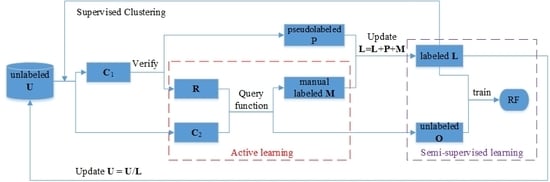
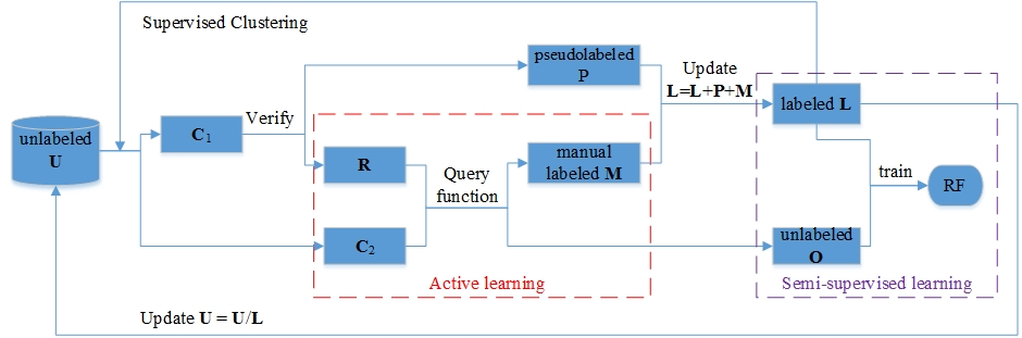
3.3. Details of ASSRF Classification

ASSRF is an iterative method that collaboratively utilizes AL and SSL to improve the classification performance. To improve the quality and quantity of labeled samples, we designed a new query function to select the most informative and diverse samples for manual labeling, and assigned pseudolabels to the samples with high classification confidence. In this way, the labeled samples would contribute SSL to obtain more accurate class probability distribution, which would improve the accuracy of the model at next iteration. The ASSRF classification included the following steps.

Initialization part (step 1):

(1)

Set the pseudolabeled data P and manually labeled data M as empty. Initial labeled data is set to L, train the random forest RF on the initial labeled data L.

Clustering part (steps 2–3):

(2)

Use Algorithm 1 to divide the unlabeled data U into many pure clusters.

(3)

The clusters that contain labeled samples are merged into set C₁, and the clusters that do not contain labeled samples are merged into set C₂.

Verification part (steps 4–5):

(4)

Train a temporary random forest rf_m on labeled data L.

(5)

The samples in set C₁ are classified by rf_m, and g samples with high classification confidence are assigned with pseudolabels. Let g samples form a set P, and let R = C₁/P.

AL part (steps 6–7):

(6)

Let the candidate pool S = C₂ ∪ R.

(7)

Use the query function DUSSC to select h samples from set S for manual labeling. Let h manually labeled samples form a set M.

SSL part (steps 8–12):

(8)

Let O = S/M, and update L: L = L ∪ P ∪ M.

(9)

Use random forest RF to classify the samples in O and obtain the probability that each sample belongs to each class.

(10)

Compute the margin vector of each sample in O by using Equation (3).

(11)

Calculate the probability distribution of each sample in O by using Equation (8), and we assign a random class label to each sample by using the probability distribution.

(12)

Use data L and O to retrain each tree in RF.

(13)

Update the unlabeled data U: U = U/L.

(14)

Repeat the steps 2 to 13 multiple times to obtain the final random forest RF.

The detailed procedure for ASSRF classification is described in Algorithm 2.

Algorithm 2 Active semi-supervised random forest classification

Input: a training data set D containing labeled pixels L and unlabeled pixels U, the size of the forest N, the batch size h for active learning, the batch size of the pseudolabeled samples g, an initial temperature T0 and a cooling function c(T, m). Initialization: the manually labeled data M = Ø and the pseudolabeled data P = Ø. 1: Train the random forest: RF ⟵ trainRF(L). 2: Set epoch: m = 0. 3: Repeat 4: Obtain the current temperature Tm+1 ⟵ c(T, m); 5: Set m ⟵ m+1; 6: Divide data U into C1 and C2 based on Algorithm 1; 7: Train temporary random forest rfm: rfm ⟵ trainRF(L); 8: Classify the samples in C1 by using rfm; 9: Select g samples with the highest-class probabilities from C1, and give them pseudolabels. Let g samples form a set P, and R = C1/P; 10: Query h most informative samples (M) from S (S = C2 ∪ R) by SSCDU for manual labeling; 11: Let O = S/M and update L = L ∪ P ∪ M; 12: ∀ x∈O, obtain the class probability p(i|x) by using RF to classify each sample x; 13: ∀ x∈O, compute the margin $g\left(\mathrm{x}\right)$ by using Equation (3); 14: ∀ x∈O, k∈Y: compute p*(k|x) by using Equation (8); 15: For n =1 to N do 16:  ∀ x∈O: Assign a random label y’ from the p*(k|x) distribution. 17:  Set Xn = L ∪ {(x, y’)|x∈O}; 18:  Retrain the tree: fn ⟵ trainTree(Xn); 19: End for 20: Update U = U/L; 21: Until epoch rounds are reached; 22: Output: the forest RF.

4. Experimental Results and Analysis

4.1. Hyperspectral Image Data Sets

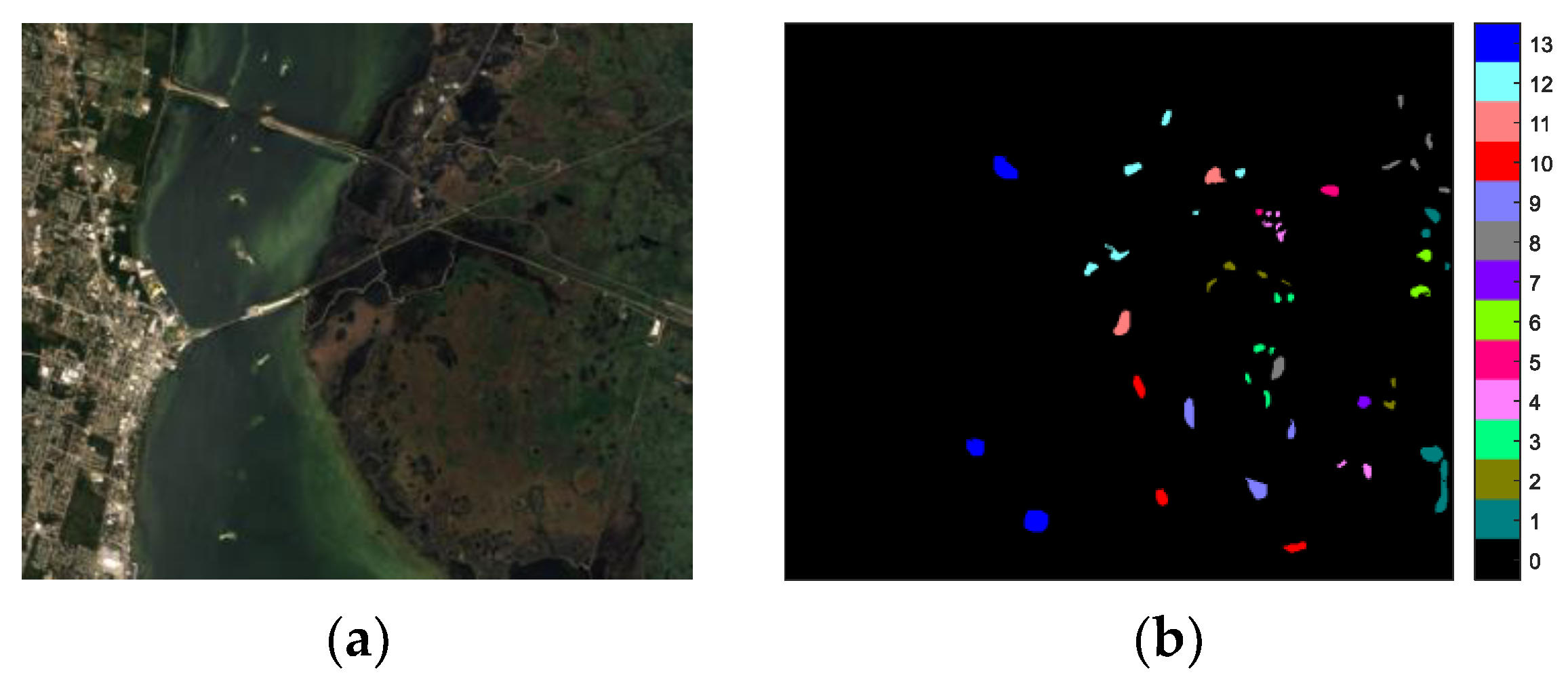
To evaluate the performance of the proposed methods, we used three public HSI data sets in our experiments.

(1)

The Kennedy Space Center (KSC) data was acquired by the NASA Airborne Visible Infrared Imaging Spectrometer sensor over the KSC, Florida, on 23 March 1996. The original data has 224 spectral bands. We used only 176 bands for our experiments because water absorption bands and bands with low signal-to-noises were excluded. The data set contained 13 classes with a size of 512 pixels × 614 pixels and the spatial resolution was 18 m/pixel. There were a total of 5211 labeled pixels in the data set.

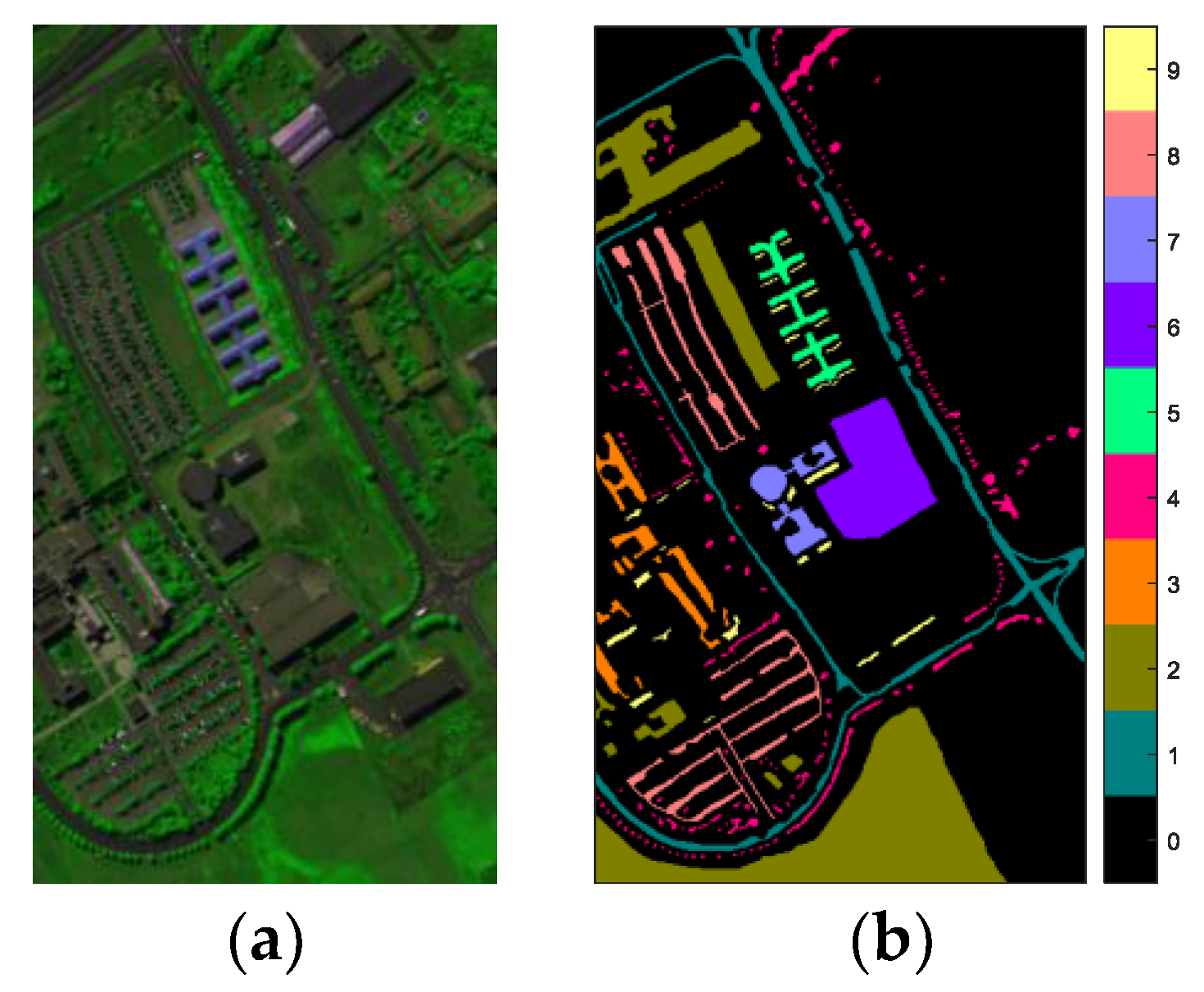
(2)

The Pavia University (PaviaU) data was obtained by the Reflective Optics Spectrographic Imaging System over an urban scene by Pavia University, Italy, in 2001. There were 115 spectral bands with wavelengths ranging from 0.43 to 0.86 μm. We chose 103 bands for the experiments after removing 12 noisy and water absorption bands. This data set had a size of 610 pixels × 340 pixels with a spatial resolution of 1.3 m/pixel. A total of 42,776 pixels covering nine classes were labeled.

(3)

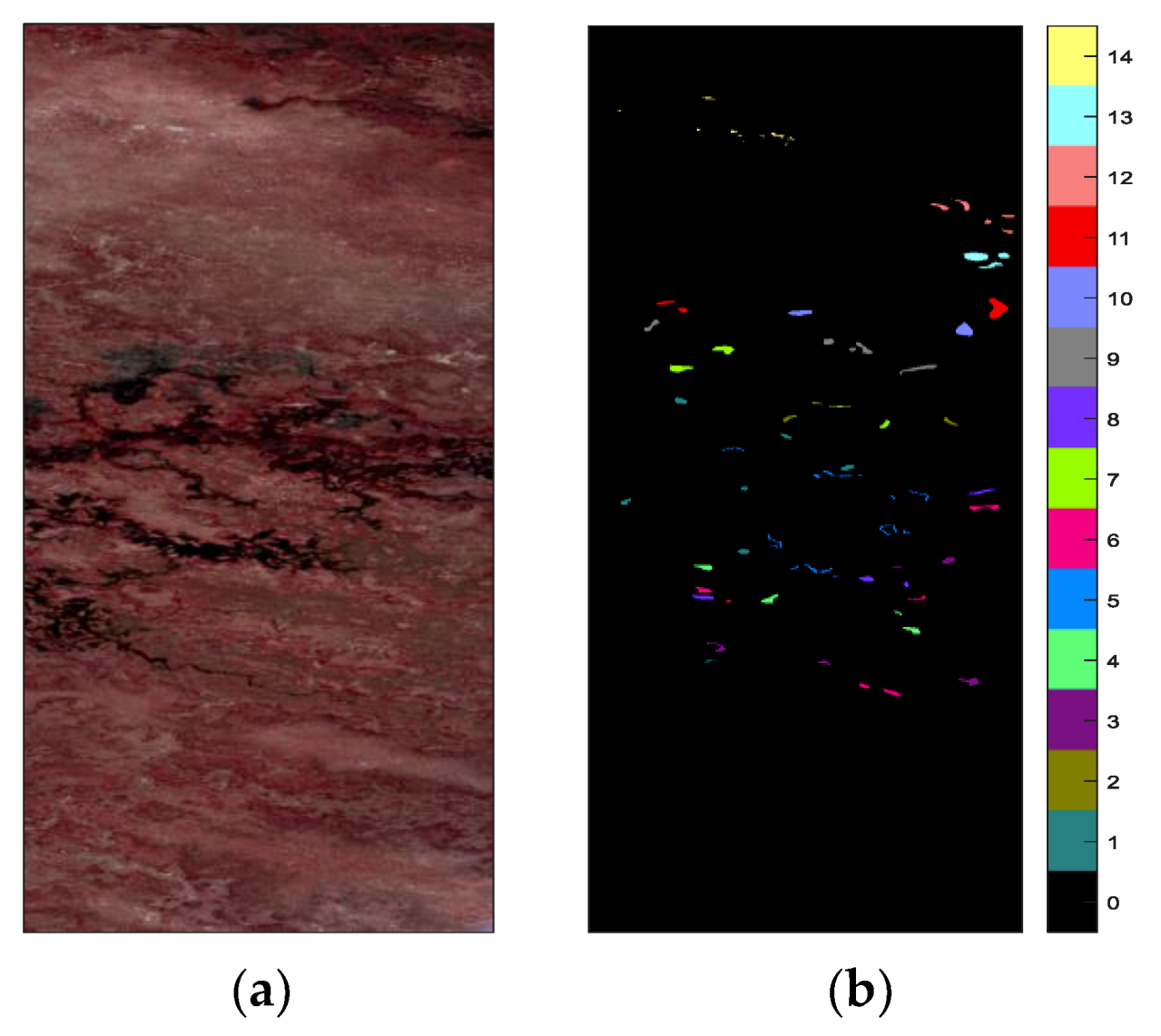
The Botswana (BOT) data was obtained by the NASA Earth Observing-1 satellite over the Okavango Delta, Botswana, on 11 May 2001. The original data has 242 bands. After removing uncalibrated and noisy bands, the remaining 145 bands were used in the experiments. The BOT data set was 1476 pixels × 256 pixels in size and had a spatial resolution of 30 m/pixel. There were 3248 labeled pixels covering 14 classes in total.

Detailed class name and number on these three data sets are shown in

Table 1. Hyperspectral data information for KSC, PaviaU and BOT.

Class No.	Kennedy Space Center (KSC)		Pavia University (PaviaU)		Botswana (BOT)
	Class Name	#Pixels	Class Name	#Pixels	Class Name	#Pixels
1	Scrub	761	Asphalt	6631	Water	270
2	Willow	243	Meadows	18,649	Hippo grass	101
3	CP hammock	256	Gravel	2099	Floodplain grass1	251
4	CP/Oak	252	Trees	3064	Floodplain grass2	215
5	Slash pine	161	Metal Sheets	1345	Reeds1	269
6	Oak/Broadleaf	229	Bare Soil	5029	Riparian	269
7	Hardwood swamp	105	Bitumen	1330	Firescar2	259
8	Graminoid marsh	431	Bricks	3682	Island interior	203
9	Spartina marsh	520	Shadows	947	Acacia woodlands	314
10	Cattail marsh	404			Acacia shrublands	248
11	Salt marsh	419			Acacia grasslands	305
12	Mud flats	503			Short mopane	181
13	Water	927			Mixed mopane	268
14					Exposed soils	95

. The three-band pseudocolor images of the three hyperspectral data sets and their corresponding reference maps are illustrated in Figure 1, Figure 2 and Figure 3.

4.2. Experimental Setup

In each hyperspectral data set, we randomly divided the available samples into two parts (60% for training and 40% for testing). For the training data, we randomly selected 10 samples for each class as the initial labeled samples. The remaining samples were used as unlabeled for active learning [43].

Several parameters need to be set in ASSRF classification. The random subspace ratio m was set to the square root of the number of spectral bands, which is a default value for RF [16]. The size of the forest N was set to 500, a reasonable value according to [9]. The parameter g, which was used to control the number of samples for pseudolabeling at each iteration, was set to 10. Following Amini et al. [47], the parameter α in Equation (8) (the contribution of the unlabeled data in the training process) was set to 0.15, while parameter β, which controls the strength of the spectral-spatial constraint, was intuitively moderate and set to 0.5 after several trials. In our parameter sensitivity analysis, we would analyze the influence of these parameters on the classification performance.

The parameters of DA were set following Amini et al. [47]; i.e., the iteration epoch was set to 20 and the simple exponential cooling function in Equation (13) was adopted to compute the parameter T in Equation (8), where T₀ = 5 is the initial temperature and T_c = 5 is a cooling constant value:

$$T=T_0\times \exp \left(\frac{-\left(epoch-1\right)}{T_c}\right).$$

(13)

The parameter h is used to control the number of samples that need to be manually labeled at each iteration. Many researchers [42,43,48] have investigated this parameter, and following Wang et al. [43], we selected 10 as the batch size for our experiments.

We first compared ASSRF classification with RF and SSRF classification. In ASSRF classification, 10 samples were selected for manual labeling at each iteration, and a total of 200 samples were manually labeled after 20 iterations. To test the effectiveness of active learning, we used two types of training data for training the RF and SSRF. The first type contained only the initial labeled samples. The second type contained the initial labeled samples and 200 randomly selected labeled samples. RF₁ and SSRF₁ represent the classifiers that were trained on the first type of training data. RF₂ and SSRF₂ represent the classifiers that were trained on the second type of training data.

We then compared ASSRF classification with other state-of-the-art methods. These methods include CASSL [42], DRDbSSAL [43], MCLU-ECBD (multi-class level uncertainty enhanced clustering-based diversity) [48], MS-cSV (margin sampling by closest support vectors) [54,63], and EQB (entropy query by bagging) [54,63]. The DRDbSSAL and CASSL methods combine AL and SSL and both use the MCLU-ECBD query function. MS-cSV is a margin sampling method based on closest support vectors. EQB is an extension of the algorithm for QBC. The experimental results from Volpi et al. [63] showed that EQB is superior to MS-cSV in most cases. For all the compared algorithms, we used the default parameter settings in the corresponding papers.

Three measures, including average accuracy (AA), overall accuracy (OA), and the kappa coefficient (k), were used evaluate the performance of the different methods. For each method, ten runs of experiments were executed on each data set to obtain the average results.

4.3. Comparison with RF and SSRF

Table 2. Class-specific accuracies, overall accuracies (OAs), average accuracies (AAs), and Kappa coefficients (in %) obtained by different methods when applied to the KSC data set.

Class No.	RF1	RF2	SSRF1	SSRF2	ASSRF
1	85.30 ± 4.45	91.81 ± 3.05	93.06 ± 2.55	94.14 ± 0.65	97.11 ± 0.93
2	76.39 ± 5.64	79.18 ± 3.97	80.52 ± 3.87	82.06 ± 2.34	89.12 ± 3.18
3	87.55 ± 5.51	89.02 ± 4.28	86.27 ± 3.95	90.49 ± 2.99	92.05 ± 2.42
4	46.70 ± 10.14	57.90 ± 13.84	62.40 ± 9.01	69.40 ± 4.35	82.44 ± 2.30
5	51.41 ± 10.71	51.41 ± 8.28	53.91 ± 7.59	55.47 ± 5.67	71.81 ± 7.41
6	45.49 ± 11.33	44.29 ± 8.08	48.90 ± 5.11	47.14 ± 5.16	67.03 ± 4.50
7	90.00 ± 7.59	90.00 ± 4.74	89.05 ± 6.16	88.81 ± 5.27	90.21 ± 3.66
8	53.48 ± 10.84	65.35 ± 9.64	80.58 ± 9.16	80.87 ± 3.95	92.77 ± 1.57
9	80.58 ± 5.04	86.54 ± 5.69	89.76 ± 4.94	93.61 ± 2.27	92.90 ± 4.82
10	72.24 ± 7.50	80.68 ± 5.69	87.27 ± 2.77	89.44 ± 4.25	95.86 ± 3.77
11	91.86 ± 2.79	92.81 ± 2.84	96.35 ± 2.53	96.35 ± 2.14	97.01 ± 0.90
12	74.43 ± 7.17	79.50 ± 7.12	84.63 ± 4.69	87.36 ± 2.95	86.84 ± 3.36
13	99.16 ± 0.54	99.11 ± 0.58	99.27 ± 0.58	99.23 ± 0.45	99.29 ± 0.47
OA	78.33 ± 1.46	82.76 ± 0.51	86.19 ± 0.91	87.91 ± 0.52	91.90 ± 0.65
AA	73.45 ± 1.73	77.53 ± 0.75	80.92 ± 0.84	82.77 ± 0.69	88.46 ± 0.88
kappa	75.87 ± 1.64	80.78 ± 0.59	84.62 ± 1.01	86.53 ± 0.58	90.97 ± 0.72

,

Table 3. Class-specific accuracies, OAs, AAs, and Kappa coefficients (in %) obtained by different methods when applied to the PaviaU data set.

Class No.	RF1	RF2	SSRF1	SSRF2	ASSRF
1	67.68 ± 5.50	79.83 ± 4.18	85.38 ± 1.79	86.79 ± 1.97	89.77 ± 1.20
2	55.52 ± 6.67	90.47 ± 3.24	95.98 ± 1.56	96.52 ± 0.97	97.17 ± 0.50
3	53.11 ± 9.48	44.60 ± 11.06	53.37 ± 5.12	51.45 ± 8.33	59.64 ± 6.70
4	86.37 ± 6.84	79.71 ± 8.25	85.33 ± 3.52	82.97 ± 4.37	87.28 ± 1.54
5	98.98 ± 0.26	98.36 ± 0.51	98.20 ± 0.76	98.16 ± 0.77	97.79 ± 0.54
6	56.95 ± 10.49	45.22 ± 8.96	45.77 ± 6.38	50.34 ± 4.68	56.04 ± 3.95
7	76.86 ± 14.91	66.65 ± 14.60	73.40 ± 4.94	77.86 ± 4.19	73.61 ± 2.93
8	67.87 ± 8.47	79.77 ± 7.15	80.21 ± 4.04	84.61 ± 4.78	84.78 ± 5.01
9	99.97 ± 0.08	99.39 ± 0.43	99.50 ± 0.46	99.66 ± 0.40	99.37 ± 0.55
OA	63.87 ± 2.99	79.26 ± 0.87	83.67 ± 0.55	84.92 ± 0.78	86.90 ± 0.75
AA	73.70 ± 1.73	76.00 ± 1.85	79.68 ± 1.16	80.93 ± 0.98	82.82 ± 0.98
kappa	55.35 ± 3.18	72.12 ± 1.13	77.84 ± 0.81	79.53 ± 1.11	82.27 ± 1.03

and

Table 4. Class-specific accuracies, OAs, AAs, and Kappa coefficients (in %) obtained by different methods when applied to the BOT data set.

Class No.	RF1	RF2	SSRF1	SSRF2	ASSRF
1	97.87 ± 2.00	99.44 ± 0.65	98.98 ± 1.27	99.72 ± 0.45	100 ± 0.00
2	95.75 ± 2.37	92.50 ± 5.53	96.25 ± 4.29	97.50 ± 4.08	93.75 ± 4.29
3	89.60 ± 6.10	90.30 ± 4.81	92.90 ± 3.76	95.00 ± 2.36	100 ± 0.00
4	87.09 ± 2.42	88.26 ± 3.26	92.33 ± 3.25	93.49 ± 2.91	99.76 ± 0.49
5	77.57 ± 4.60	78.50 ± 3.99	81.12 ± 3.73	80.09 ± 3.47	90.93 ± 2.46
6	49.07 ± 10.51	53.46 ± 7.14	63.93 ± 5.24	74.30 ± 6.80	80.65 ± 3.61
7	90.38 ± 2.91	94.47 ± 2.71	97.48 ± 1.31	97.57 ± 1.54	98.93 ± 0.85
8	86.42 ± 9.33	90.12 ± 4.39	94.44 ± 2.62	95.93 ± 2.47	99.87 ± 0.39
9	64.64 ± 12.20	71.20 ± 7.87	82.16 ± 4.67	85.36 ± 2.36	95.12 ± 1.79
10	74.65 ± 12.13	81.72 ± 9.55	85.66 ± 6.38	87.47 ± 4.98	95.25 ± 2.38
11	83.28 ± 5.56	87.30 ± 4.66	91.48 ± 3.67	92.54 ± 2.43	96.89 ± 1.89
12	92.64 ± 5.12	92.64 ± 4.72	92.92 ± 2.81	95.14 ± 1.76	95.14 ± 2.95
13	69.44 ± 6.78	81.87 ± 6.95	87.95 ± 4.07	87.38 ± 3.67	93.74 ± 2.45
14	97.63 ± 1.94	97.63 ± 1.94	97.11 ± 3.39	99.21 ± 1.27	93.16 ± 3.96
OA	80.42 ± 0.78	84.16 ± 1.22	88.56 ± 0.70	90.46 ± 0.65	95.34 ± 0.37
AA	82.57 ± 0.72	85.67 ± 0.97	89.62 ± 0.73	91.48 ± 0.65	95.23 ± 0.40
kappa	78.83 ± 0.84	82.85 ± 1.32	87.79 ± 0.88	89.66 ± 0.71	94.84 ± 0.40

show the class-specific accuracies, AAs, OAs, and kappa coefficients obtained by the different methods when applied to the KSC, PaviaU, and BOT data sets, respectively. The best results for different method are highlighted in bold.

We could obtain several findings from Table 2, Table 3 and Table 4. First, ASSRF achieved the best class-specific accuracy in most cases. Specifically, ASSRF achieved 11, 5, and 11 best class-specific accuracies on KSC, PaviaU, and BOT data sets, respectively. The class-specific accuracies of the other classes obtained by ASSRF were slightly lower than the best results. Second, among all the data sets, ASSRF achieved the best results on OAs, AAs, and the kappa coefficients; SSRF obtained the second-best results; and RF obtained the worst results. Third, compared with RF₁ and SSRF₁ classification, RF₂ and SSRF₂ classification exhibited improved performance on OA, AA, and kappa coefficient since RF₂ and SSRF₂ not only use the initial labeled samples but also use the extra 200 randomly labeled samples to train the classifiers. Fourth, SSRF classification performed better than RF classification, because it benefits from a semi-supervised method that acquires the probability distribution of the training samples. Fifth, ASSRF significantly improved the classification performance because it used a unified framework that combines Al and SSL to train the classifier. Compared with SSRF₁ classification, we could see that SSRF₂ improved the accuracy slightly, while ASSRF improved it significantly. Although both SSRF₂ and ASSRF classification used the extra 200 labeled samples for training, the 200 labeled samples used in SSRF₂ and ASSRF classification were different. The 200 labeled samples used in SSRF₂ were randomly selected from the training set at the beginning of training the classifier, while those in ASSRF were selected in an iterative manner by our proposed active learning method. The classification maps for different methods on KSC and PaviaU data sets are depicted in Figure 4 and Figure 5, respectively.

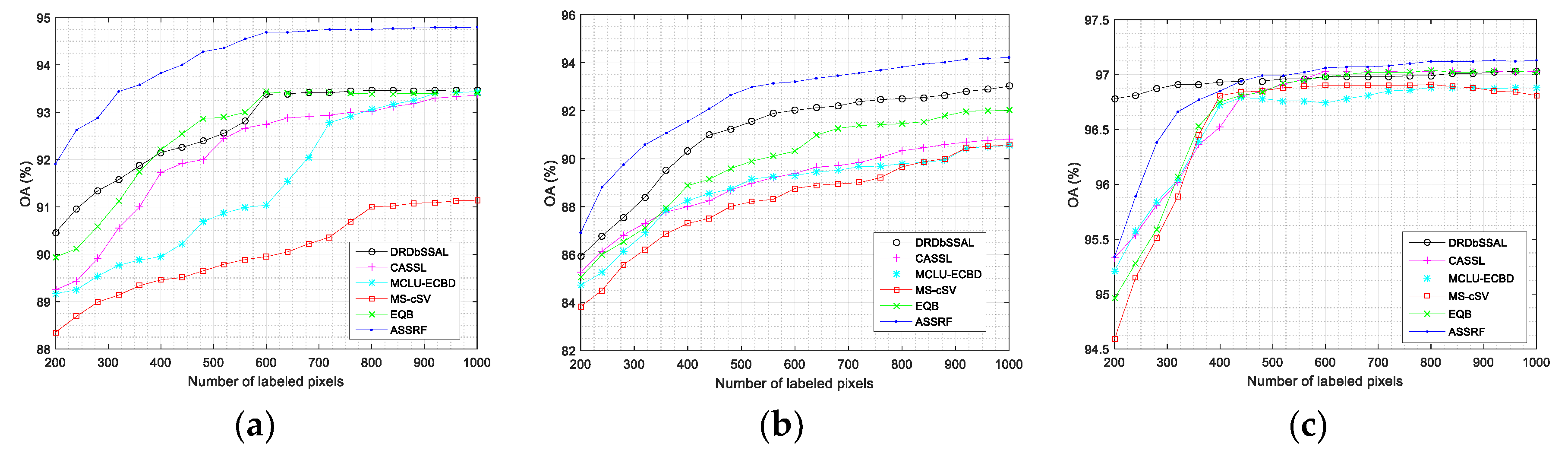
4.4. Comparison with Other State-Of-The-Art Methods

In this section, we compared ASSRF with other state-of-the-art methods, including DRDbSSAL, CASSL, MCLU-ECBD, MS-cSV, and EQB, which were introduced in Section 4.2. To verify the impact of the number of AL-labeled samples on the performance of different algorithms, we calculated the average OA on the testing sets over 10 runs until the number of labeled samples expanded to 1000. Figure 6 shows the OAs obtained from the testing sample sets.

Table 5. Proposed ASSRF method versus other state-of-the-art methods based on a performance comparison showing the OA (in %) obtained from the KSC data set.

Data Size	DRDbSSAL	CASSL	MCLU-ECBD	MS-cSV	EQB	ASSRF
200	90.58 ± 0.76	89.24 ± 0.66	89.15 ± 0.97	88.35 ± 0.71	90.00 ± 0.23	91.90 ± 0.65
400	92.22 ± 0.87	91.76 ± 0.83	89.96 ± 0.79	89.50 ± 0.54	92.23 ± 0.38	93.81 ± 0.32
600	93.43 ± 0.10	92.77 ± 0.21	91.08 ± 0.46	89.96 ± 0.91	93.43 ± 0.23	94.68 ± 0.39
800	93.48 ± 0.04	93.03 ± 0.23	93.05 ± 0.20	91.03 ± 0.49	93.40 ± 0.10	94.76 ± 0.24
1000	93.47 ± 0.06	93.37 ± 0.31	93.46 ± 0.10	91.15 ± 0.65	93.41 ± 0.16	94.79 ± 0.21

,

Table 6. Proposed ASSRF method versus other state-of-the-art methods based on a performance comparison showing the OA (in %) obtained from the PaviaU data set.

Data Size	DRDbSSAL	CASSL	MCLU-ECBD	MS-cSV	EQB	ASSRF
200	85.97 ± 2.61	85.30 ± 0.63	84.74 ± 1.49	83.84 ± 1.96	85.07 ± 1.16	86.90 ± 0.75
400	90.37 ± 0.73	88.00 ± 1.01	88.23 ± 0.81	87.30 ± 1.33	88.89 ± 0.31	91.56 ± 0.54
600	92.04 ± 0.69	89.40 ± 1.01	89.31 ± 0.60	88.77 ± 0.95	90.32 ± 0.49	93.21 ± 0.39
800	92.54 ± 0.06	90.35 ± 0.73	89.78 ± 2.76	89.65 ± 0.69	91.48 ± 0.41	93.82 ± 0.14
1000	93.03 ± 0.07	90.83 ± 0.70	90.59 ± 2.18	90.59 ± 1.04	92.01 ± 0.34	94.19 ± 0.18

and

Table 7. Proposed ASSRF method versus other state-of-the-art methods based on a performance comparison showing the OA (in %) obtained from the BOT data set.

Data Size	DRDbSSAL	CASSL	MCLU-ECBD	MS-cSV	EQB	ASSRF
200	96.80 ± 0.41	95.33 ± 0.25	95.21 ± 0.48	94.59 ± 0.39	94.96 ± 0.35	95.34 ± 0.37
400	96.94 ± 0.12	96.72 ± 0.36	96.79 ± 0.18	96.81 ± 0.14	96.75 ± 0.19	96.81 ± 0.25
600	96.99 ± 0.00	97.03 ± 0.13	96.75 ± 0.08	96.91 ± 0.09	96.98 ± 0.13	97.06 ± 0.09
800	96.99 ± 0.01	97.03 ± 0.13	96.88 ± 0.07	96.91 ± 0.09	97.04 ± 0.11	97.12 ± 0.03
1000	97.03 ± 0.03	97.03 ± 0.13	96.88 ± 0.04	96.80 ± 0.04	97.02 ± 0.13	97.13 ± 0.02

exhibit quantitative evaluations of different algorithms on the three hyperspectral data sets.

The results in Figure 6 proved that for all compared methods on each hyperspectral data set, the average OA increased as the number of labeled samples increased. ASSRF consistently outperformed the other methods on the KSC and PaviaU data sets, no matter how many samples were manually labeled. The average OA of ASSRF on the BOT data set was slightly lower than that of DRDbSSAL when the number of labeled samples was less than 400. However, when the number of labeled samples was larger, the performance of ASSRF was slightly better than that of DRDbSSAL. The quantitative evaluations from Table 5, Table 6 and Table 7 also demonstrated that ASSRF obtained better performance than other methods. The standard deviations of the accuracies from different methods indicate that ASSRF was more robust than CASSL, MCLU-ECBD, MS-cSV, and EQB and had approximately the same robustness as DRDbSSAL.

All the methods in our experiments were implemented using MATLAB 2015b platform with 3.4GHz Intel i7-6700 CPU and 8 GB RAM.

Table 8. Training time on two hyperspectral images.

Time (s)	KSC	PaviaU
DRDbSSAL	1785.3	4751.8
CASSL	1263.5	3354.2
MCLU-ECBD	305.8	1241.7
MS-cSV	3165.8	8745.6
EQB	267.55	879.6
ASSRF	967.3	2235.3

compares the training time of each method on KSC and PaviaU data sets. The results indicate that MS-cSV is the most time-consuming method, MCLU-ECBD and EQB require the least time cost, CASSL, DRDbSSAL, and ASSRF need a medium computation time. In addition, the time cost of ASSRF was a little shorter than CASSL and DRDbSSAL. The results show that the computation time of ASSRF was acceptable.

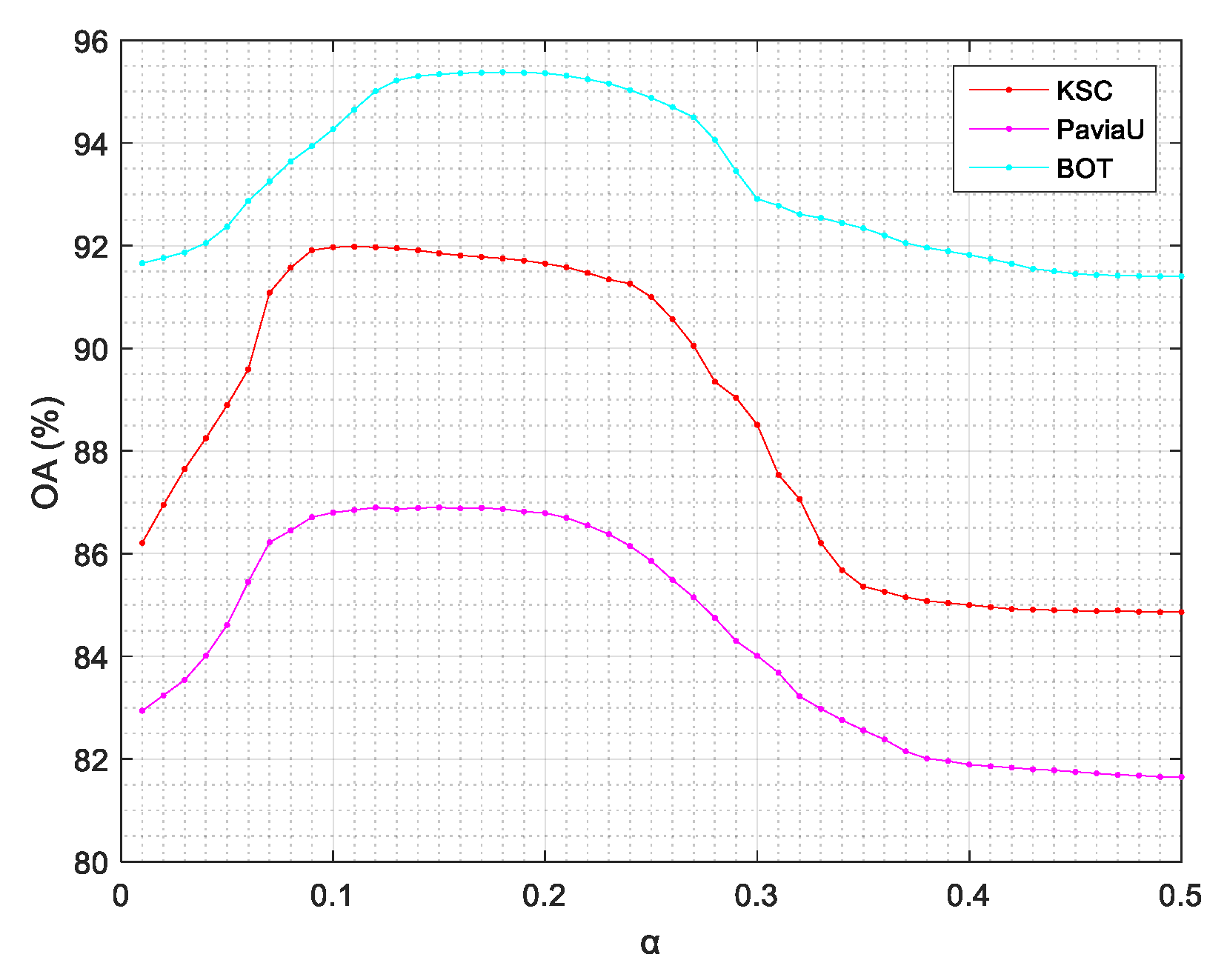
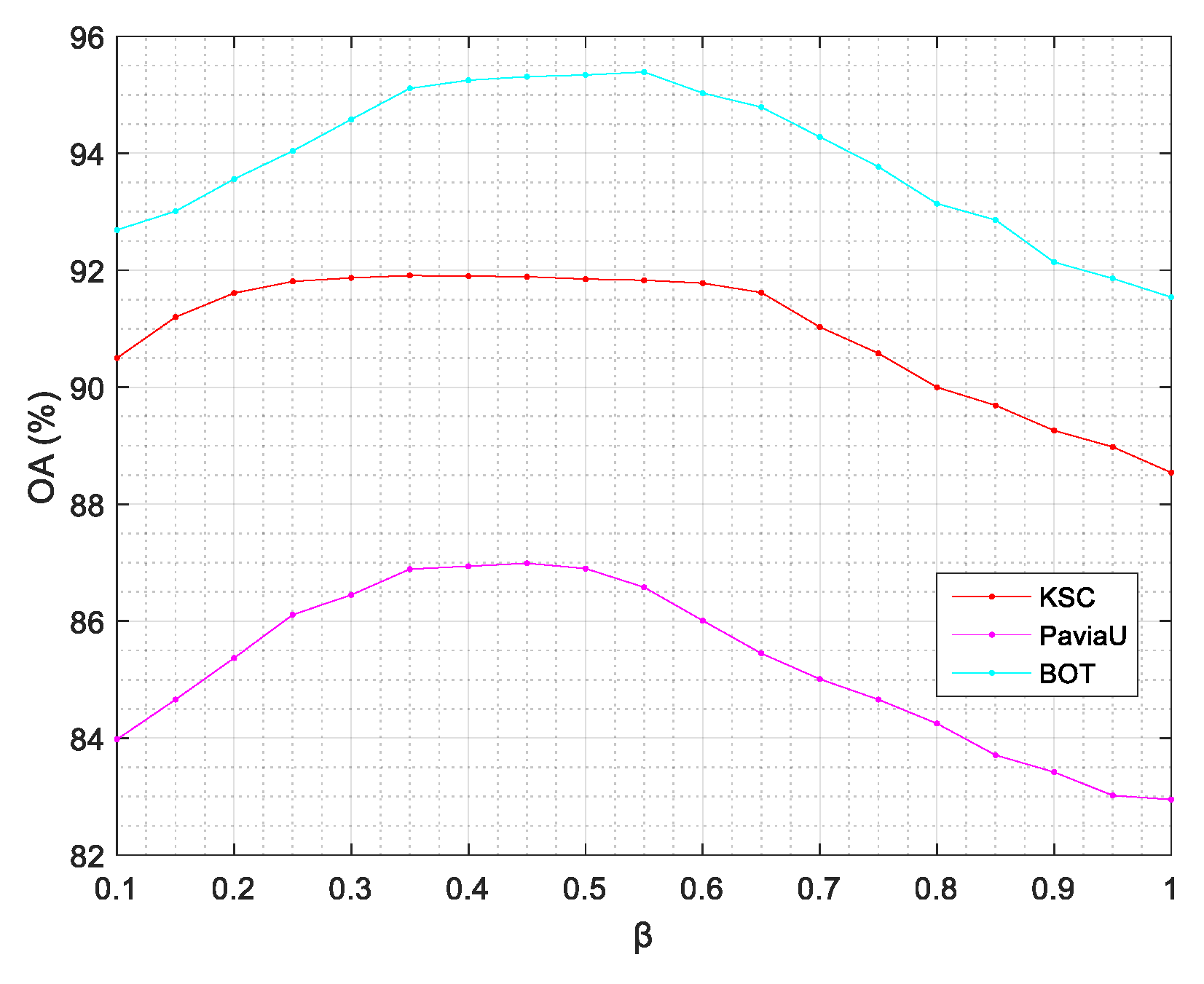
4.5. Parameter Sensitivity Analysis

As we discussed in the previous sections, the parameter α represents the contribution of the unlabeled data to the procedure of semi-supervised regularization and the parameter β represents the constraint strength of the spectral-spatial information on the decision labels. To explore the influence of these two parameters on the classification accuracy, we conducted experiments using different values of α and β. When we analyzed each parameter, the other parameters were fixed. First, we set α in the range [0.01, 0.5] with a step size of 0.01 to evaluate the overall classification accuracy. Then, we set β in the range [0.1, 1] with a step size of 0.05 to evaluate the overall classification accuracy. The influences of the parameters α and β on the classification accuracy for the three hyperspectral data sets are shown in Figure 7 and Figure 8, respectively.

Figure 7 and Figure 8 show that the accuracy of ASSRF first increased, then reached the peak value, and at last decreased or maintained this value. The main reason for these results is as follows. When α is too small, the dominant term for SSL is the labeled data, while the unlabeled data have little influence. However, when α is too large, the dominant term for SSL is the unlabeled data, which will lead to that the uncertainty becomes too large to optimize. For the parameter β, a moderate value makes the spectral-spatial constraint work better, while too-small or too-large values will result in low accuracy. Thus, the value for α should be small but not too small, and the value for β should be moderate. We conclude that the recommended value for α ranges from 0.1 to 0.25 and the recommended value for β ranges from 0.35 to 0.55.

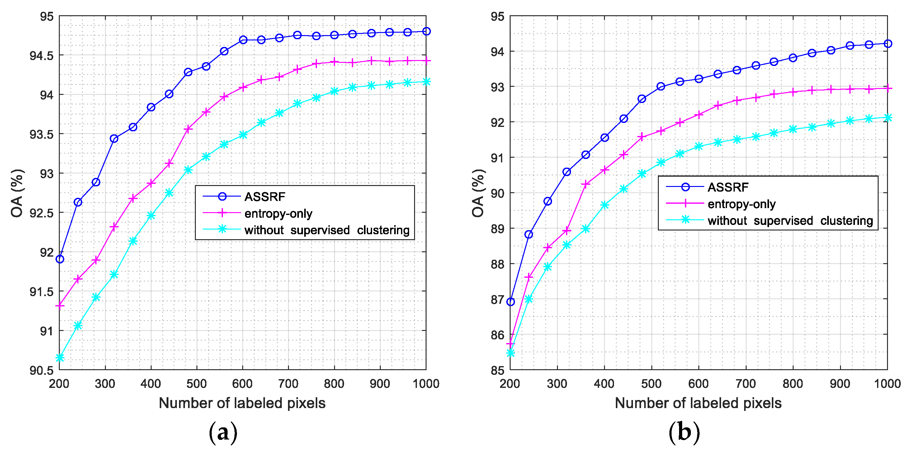
4.6. Further Analysis of ASSRF

In this section, we analyzed the contribution of two parts in ASSRF on the improvement of the classification performance. First, to evaluate the importance of spectral-spatial constraint to the query function of AL, we used the query function without spectral-spatial constraint for AL. The query function degraded from Equation (9) is described as Equation (14).

$$f\left(\mathrm{x}\right)=-{{\displaystyle \sum }}_{i=1}^K{p}_i\left(\mathrm{x}\right)\log (p_i\left(\mathrm{x}\right)).$$

(14)

Compared with Equation (9), the query function in Equation (14) only contains one part, i.e., information entropy. This method is referred to as entropy-only. We did experiments for the entropy-only method to demonstrate the importance of spectral-spatial constraint. Second, to verify the role of the supervised clustering algorithm in ASSRF, we did experiments for ASSRF without supervised clustering.

The results obtained on KSC and PaviaU data sets are illustrated in Figure 9. We could observe that both the spectral-spatial constraint and supervised k-means clustering algorithm played an important role in ASSRF, and supervised k-means clustering made more contributions to the accuracy improvement than that of the spectral-spatial constraint.

5. Discussion

The experiments on three real hyperspectral data sets revealed several interesting points.

• As shown in Section 4.3 and Section 4.4, compared with other methods, ASSRF performed better classification performance. The good performance of ASSRF could be attributed to the following three reasons. First, supervised clustering can extract the structure of the whole data and divide it into two parts, one for active learning and one for pseudolabeling. Second, the proposed query function DUSSC can select the most informative and diverse samples for manual labeling. Third, the unified framework combining AL and SSL can increase the learning performance by increasing the quantity and quality of the labeled samples.
• The results from Table 8 show that the computation time of ASSRF was acceptable. Several reasons could explain this result. First, the training process of each tree in the forest was parallel. Second, the time complexity of k-means algorithm was linear, and the time cost of supervised k-means method was at most m times the k-means, where m is the number of labeled samples. Third, the process of DA-based SSL could be solved as an analytical solution, which made the computation of SSL is on line.
• The parameter analysis in Section 4.5 shows that ASSRF was robust to parameters. According to our experiments, the recommended value for α ranges from 0.1 to 0.25 and the recommended value for β ranges from 0.35 to 0.55.
• The experimental results from Section 4.6 show that both the spectral-spatial constraint and supervised k-means clustering algorithm played an important role in ASSRF. This is mainly because that ASSRF without supervised clustering does not provide enough pseudolabeled samples for the classification model. In other words, the model focuses on informative samples but ignores the samples easy, which are to classify, leading to the bias of the model and affecting the final accuracy. Another finding was that the importance of spectral-spatial constraint was less than supervised clustering.
• ASSRF is a unified framework combing AL and SSL into random forest. Generally, ASSRF can be used for any data represented in vector form. However, we added spectral-spatial constraints into query function for AL, where the spectral-spatial constraint utilized the neighborhood structure information of images. So, for usual data represented in vector form, the entropy-only-based ASSRF was appropriate.

6. Conclusions

In this paper, we proposed an active semi-supervised random forest (ASSRF) classifier for HSI classification. ASSRF collaboratively utilized active learning and semi-supervised learning to improve the final classification performance. To mine the structure of the whole data, supervised clustering was used to categorize the unlabeled data. In addition, a new query function called DUSSC was proposed to select the most informative and diverse samples for manual labeling. The proposed method was compared with random forest, semi-supervised random forest, and other state-of-the-art methods on three public hyperspectral data sets. Experiments on KSC, PaviaU, and BOT data sets demonstrated that compared with state-of-the-art method, the proposed ASSRF significantly improved the classification performance, especially on KSC and PaviaU data sets. In addition, the computational cost of ASSRF was moderate and acceptable. At last, the proposed method was robust to parameters.

In future work, we would investigate the proposed unified framework on rotation forest [71]. Furthermore, we would consider introducing morphological properties into the proposed classifier for HSI classification.

References

1. Zare, A.; Bolton, J.; Gader, P.; Schatten, M. Vegetation mapping for landmine detection using long-wave hyperspectral imagery. IEEE Trans. Geosci. Remote Sens. 2008, 46, 172–178. [Google Scholar] [CrossRef]
2. Fu, Y.; Zhao, C.; Wang, J.; Jia, X.; Yang, G.; Song, X.; Feng, H. An improved combination of spectral and spatial features for vegetation classification in hyperspectral images. Remote Sens. 2017, 9, 261. [Google Scholar] [CrossRef] [Green Version]
3. Jiao, L.; Sun, W.; Yang, G.; Ren, G.; Liu, Y. A hierarchical classification framework of satellite multispectral/hyperspectral images for mapping coastal wetlands. Remote Sens. 2019, 11, 2238. [Google Scholar] [CrossRef] [Green Version]
4. Moeini Rad, A.; Abkar, A.A.; Mojaradi, B. Supervised distance-based feature selection for hyperspectral target detection. Remote Sens. 2019, 11, 2049. [Google Scholar] [CrossRef] [Green Version]
5. Wei, L.; Huang, C.; Zhong, Y.; Wang, Z.; Hu, X.; Lin, L. Inland waters suspended solids concentration retrieval based on PSO-LSSVM for UAV-borne hyperspectral remote sensing imagery. Remote Sens. 2019, 11, 1455. [Google Scholar] [CrossRef] [Green Version]
6. Patra, S.; Bruzzone, L. A novel SOM-SVM-based active learning technique for remote sensing image classification. IEEE Trans. Geosci. Remote Sens. 2014, 52, 6899–6910. [Google Scholar] [CrossRef]
7. Mou, L.; Ghamisi, P.; Zhu, X.X. Deep recurrent neural networks for hyperspectral image classification. IEEE Trans. Geosci. Remote Sens. 2017, 55, 3639–3655. [Google Scholar] [CrossRef] [Green Version]
8. Seydgar, M.; Alizadeh Naeini, A.; Zhang, M.; Li, W.; Satari, M. 3-D convolution-recurrent networks for spectral-spatial classification of hyperspectral images. Remote Sens. 2019, 11, 883. [Google Scholar] [CrossRef] [Green Version]
9. Belgiu, M.; Drăgu, L. Random forest in remote sensing: A review of applications and future directions. ISPRS J. Photogramm. Remote Sens. 2016, 114, 24–31. [Google Scholar] [CrossRef]
10. Zhang, Y.; Cao, G.; Li, X.; Wang, B. Cascaded random forest for hyperspectral image classification. IEEE J. Sel. Top. Appl. Earth Obs. Remote Sens. 2018, 11, 1082–1094. [Google Scholar] [CrossRef]
11. Xia, J.; Ghamisi, P.; Yokoya, N.; Iwasaki, A. Random forest ensembles and extended multiextinction profiles for hyperspectral image classification. IEEE Trans. Geosci. Remote Sens. 2018, 56, 202–216. [Google Scholar] [CrossRef] [Green Version]
12. Rajan, S.; Ghosh, J.; Crawford, M.M. An active learning approach to hyperspectral data classification. IEEE Trans. Geosci. Remote Sens. 2008, 46, 1231–1242. [Google Scholar] [CrossRef]
13. Kong, Y.; Wang, X.; Cheng, Y.; Chen, C.L.P. Hyperspectral imagery classification based on semi-supervised broad learning system. Remote Sens. 2018, 10, 685. [Google Scholar] [CrossRef] [Green Version]
14. Crawford, M.M.; Tuia, D.; Yang, H.L. Active learning: Any value for classification of remotely sensed data? Proc. IEEE 2013, 101, 593–608. [Google Scholar] [CrossRef] [Green Version]
15. Tuia, D.; Volpi, M.; Copa, L.; Kanevski, M.; Muñoz-Marí, J. A survey of active learning algorithms for supervised remote sensing image classification. IEEE J. Sel. Top. Signal Process. 2011, 5, 606–617. [Google Scholar] [CrossRef]
16. Breiman, L. Random forests. Mach. Learn. 2001, 45, 5–32. [Google Scholar] [CrossRef] [Green Version]
17. Mahdianpari, M.; Salehi, B.; Mohammadimanesh, F.; Motagh, M. Random forest wetland classification using ALOS-2 L-band, RADARSAT-2 C-band, and TerraSAR-X imagery. ISPRS J. Photogramm. Remote Sens. 2017, 130, 13–31. [Google Scholar] [CrossRef]
18. Chan, J.C.W.; Paelinckx, D. Evaluation of random forest and Adaboost tree-based ensemble classification and spectral band selection for ecotope mapping using airborne hyperspectral imagery. Remote Sens. Environ. 2008, 112, 2999–3011. [Google Scholar] [CrossRef]
19. Ghimire, B.; Rogan, J.; Miller, J. Contextual land-cover classification: Incorporating spatial dependence in land-cover classification models using random forests and the Getis statistic. Remote Sens. Lett. 2010, 1, 45–54. [Google Scholar] [CrossRef] [Green Version]
20. Ham, J.S.; Chen, Y.; Crawford, M.M.; Ghosh, J. Investigation of the random forest framework for classification of hyperspectral data. IEEE Trans. Geosci. Remote Sens. 2005, 43, 492–501. [Google Scholar] [CrossRef] [Green Version]
21. Mellor, A.; Boukir, S.; Haywood, A.; Jones, S. Exploring issues of training data imbalance and mislabelling on random forest performance for large area land cover classification using the ensemble margin. ISPRS J. Photogramm. Remote Sens. 2015, 105, 155–168. [Google Scholar] [CrossRef]
22. Pal, M. Random forest classifier for remote sensing classification. Int. J. Remote Sens. 2005, 26, 217–222. [Google Scholar] [CrossRef]
23. Rodriguez-Galiano, V.F.; Ghimire, B.; Rogan, J.; Chica-Olmo, M.; Rigol-Sanchez, J.P. An assessment of the effectiveness of a random forest classifier for land-cover classification. ISPRS J. Photogramm. Remote Sens. 2012, 67, 93–104. [Google Scholar] [CrossRef]
24. Xia, J.; Liao, W.; Chanussot, J.; Du, P.; Song, G.; Philips, W. Improving random forest with ensemble of features and semisupervised feature extraction. IEEE Geosci. Remote Sens. Lett. 2015, 12, 1471–1475. [Google Scholar]
25. Behnamian, A.; Millard, K.; Banks, S.N.; White, L.; Richardson, M.; Pasher, J. A systematic approach for variable selection with random rorests: Achieving stable variable importance values. IEEE Geosci. Remote Sens. Lett. 2017, 14, 1988–1992. [Google Scholar] [CrossRef] [Green Version]
26. Romaszewski, M.; Głomb, P.; Cholewa, M. Semi-supervised hyperspectral classification from a small number of training samples using a co-training approach. ISPRS J. Photogramm. Remote Sens. 2016, 121, 60–76. [Google Scholar] [CrossRef]
27. Zhang, X.; Song, Q.; Liu, R.; Wang, W.; Jiao, L. Modified co-training with spectral and spatial views for semisupervised hyperspectral image classification. IEEE J. Sel. Top. Appl. Earth Obs. Remote Sens. 2014, 7, 2044–2055. [Google Scholar] [CrossRef]
28. Dopido, I.; Li, J.; Marpu, P.R.; Plaza, A.; Bioucas Dias, J.M.; Benediktsson, J.A. Semisupervised self-learning for hyperspectral image classification. IEEE Trans. Geosci. Remote Sens. 2013, 51, 4032–4044. [Google Scholar] [CrossRef] [Green Version]
29. Mianji, F.A.; Gu, Y.; Zhang, Y.; Zhang, J. Enhanced self-training superresolution mapping technique for hyperspectral imagery. IEEE Geosci. Remote Sens. Lett. 2011, 8, 671–675. [Google Scholar] [CrossRef]
30. Camps-Valls, G.; Bandos Marsheva, T.V.; Zhou, D. Semi-supervised graph-based hyperspectral image classification. IEEE Trans. Geosci. Remote Sens. 2007, 45, 3044–3054. [Google Scholar] [CrossRef]
31. Zhang, Y.; Cao, G.; Shafique, A.; Fu, P. Label propagation ensemble for hyperspectral image classification. IEEE J. Sel. Top. Appl. Earth Obs. Remote Sens. 2019, 12, 3623–3636. [Google Scholar] [CrossRef]
32. Gómez-Chova, L.; Camps-Valls, G.; Muñoz-Mari, J.; Calpe, J. Semisupervised image classification with Laplacian support vector machines. IEEE Geosci. Remote Sens. Lett. 2008, 5, 336–340. [Google Scholar] [CrossRef]
33. Yang, L.; Yang, S.; Jin, P.; Zhang, R. Semi-supervised hyperspectral image classification using spatio-spectral laplacian support vector machine. IEEE Geosci. Remote Sens. Lett. 2013, 11, 651–655. [Google Scholar] [CrossRef]
34. Tomašev, N.; Buza, K. Hubness-aware kNN classification of high-dimensional data in presence of label noise. Neurocomputing 2015, 160, 157–172. [Google Scholar] [CrossRef] [Green Version]
35. Buza, K. Classification of gene expression data: A hubness-aware semi-supervised approach. Comput. Methods Programs Biomed. 2016, 127, 105–113. [Google Scholar] [CrossRef] [Green Version]
36. Marussy, K.; Buza, K. SUCCESS: A new approach for semi-supervised classification of time-series. In Proceedings of the International Conference on Artificial Intelligence and Soft Computing, Zakopane, Poland, 9–13 June 2013; Springer: Berlin, Germany; pp. 437–447. [Google Scholar]
37. Peikari, M.; Salama, S.; Nofech-Mozes, S.; Martel, A.L. A Cluster-then-label semi-supervised learning approach for pathology image classification. Sci. Rep. 2018, 8, 7193. [Google Scholar] [CrossRef] [Green Version]
38. Li, J.; Bioucas-Dias, J.M.; Plaza, A. Semisupervised hyperspectral image segmentation using multinomial logistic regression with active learning. IEEE Trans. Geosci. Remote Sens. 2010, 48, 4085–4098. [Google Scholar] [CrossRef] [Green Version]
39. Munoz-Mari, J.; Tuia, D.; Camps-Valls, G. Semisupervised classification of remote sensing images with active queries. IEEE Trans. Geosci. Remote Sens. 2012, 50, 3751–3763. [Google Scholar] [CrossRef]
40. Samiappan, S.; Moorhead, R.J. Semi-supervised co-training and active learning framework for hyperspectral image classification. In Proceedings of the International Geoscience and Remote Sensing Symposium (IGARSS), Milan, Italy, 26–31 July 2015; pp. 401–404. [Google Scholar]
41. Di, W.; Crawford, M.M. Active learning via multi-view and local proximity co-regularization for hyperspectral image classification. IEEE J. Sel. Top. Signal Process. 2011, 5, 618–628. [Google Scholar] [CrossRef] [Green Version]
42. Wan, L.; Tang, K.; Li, M.; Zhong, Y.; Qin, A.K. Collaborative active and semisupervised learning for hyperspectral remote sensing image classification. IEEE Trans. Geosci. Remote Sens. 2015, 53, 2384–2396. [Google Scholar] [CrossRef]
43. Wang, Z.; Du, B.; Zhang, L.; Zhang, L.; Jia, X. A novel semisupervised active-learning algorithm for hyperspectral image classification. IEEE Trans. Geosci. Remote Sens. 2017, 55, 3071–3083. [Google Scholar] [CrossRef]
44. Zhang, Z.; Pasolli, E.; Crawford, M.M.; Tilton, J.C. An active learning framework for hyperspectral image classification using hierarchical segmentation. IEEE J. Sel. Top. Appl. Earth Obs. Remote Sens. 2016, 9, 640–654. [Google Scholar] [CrossRef]
45. Dopido, I.; Li, J.; Plaza, A.; Bioucas-Dias, J.M. Semi-supervised active learning for urban hyperspectral image classification. In Proceedings of the International Geoscience and Remote Sensing Symposium (IGARSS), Munich, Germany, 22–27 July 2012; pp. 1586–1589. [Google Scholar]
46. Leistner, C.; Saffari, A.; Santner, J.; Bischof, H. Semi-supervised random forests. In Proceedings of the IEEE International Conference on Computer Vision (ICCV), Kyoto, Japan, 27 September–4 October 2009; pp. 506–513. [Google Scholar]
47. Amini, S.; Homayouni, S.; Safari, A. Semi-supervised classification of hyperspectral image using random forest algorithm. In Proceedings of the International Geoscience and Remote Sensing Symposium (IGARSS), Quebec, Canada, 13–18 July 2014; pp. 2866–2869. [Google Scholar]
48. Demir, B.; Persello, C.; Bruzzone, L. Batch-mode active-learning methods for the interactive classification of remote sensing images. IEEE Trans. Geosci. Remote Sens. 2011, 49, 1014–1031. [Google Scholar] [CrossRef] [Green Version]
49. Lewis, D.D.; Gale, W.A. A sequential algorithm for training text classifiers. In Proceedings of the 17th Annual International ACM SIGIR Conference on Research and Development in Information Retrieval, Dublin, Ireland, 3–6 July 1994; pp. 3–12. [Google Scholar]
50. Campbell, C.; Cristianini, N.; Smola, A. Query learning with large margin classifiers. In Proceedings of the 7th International Conference on Machine Learning (ICML), Stanford, CA, USA, 29 June–2 July 2000; pp. 111–118. [Google Scholar]
51. Tong, S.; Koller, D. Support vector machine active learning with applications to text classification. J. Mach. Learn. Res. 2001, 2, 45–66. [Google Scholar]
52. Di, W.; Crawford, M.M. View generation for multiview maximum disagreement based active learning for hyperspectral image classification. IEEE Trans. Geosci. Remote Sens. 2012, 50, 1942–1954. [Google Scholar] [CrossRef]
53. Freund, Y.; Seung, H.S.; Shamir, E.; Tishby, N. Selective sampling using the query by committee algorithm. Mach. Learn. 1997, 28, 133–168. [Google Scholar] [CrossRef]
54. Tuia, D.; Ratle, F.; Pacifici, F.; Kanevski, M.F.; Emery, W.J. Active learning methods for remote sensing image classification. IEEE Trans. Geosci. Remote Sens. 2009, 47, 2218–2232. [Google Scholar] [CrossRef]
55. Zhang, Z.; Crawford, M.M. A batch-mode regularized multimetric active learning framework for classification of hyperspectral images. IEEE Trans. Geosci. Remote Sens. 2017, 55, 6594–6609. [Google Scholar] [CrossRef]
56. Shi, Q.; Du, B.; Zhang, L. Spatial coherence-based batch-mode active learning for remote sensing image classification. IEEE Trans. Image Process. 2015, 24, 2037–2050. [Google Scholar]
57. Demir, B.; Minello, L.; Bruzzone, L. An effective strategy to reduce the labeling cost in the definition of training sets by active learning. IEEE Geosci. Remote Sens. Lett. 2014, 11, 79–83. [Google Scholar] [CrossRef]
58. Xue, Z.; Zhou, S.; Zhao, P. Active learning improved by neighborhoods and superpixels for hyperspectral image classification. IEEE Geosci. Remote Sens. Lett. 2018, 15, 469–473. [Google Scholar] [CrossRef]
59. Pasolli, E.; Melgani, F.; Tuia, D.; Pacifici, F.; Emery, W.J. SVM active learning approach for image classification using spatial information. IEEE Trans. Geosci. Remote Sens. 2014, 52, 2217–2223. [Google Scholar] [CrossRef]
60. Guo, J.; Zhou, X.; Li, J.; Plaza, A.; Prasad, S. Superpixel-based active learning and online feature importance learning for hyperspectral image analysis. IEEE J. Sel. Top. Appl. Earth Obs. Remote Sens. 2017, 10, 347–359. [Google Scholar] [CrossRef]
61. Patra, S.; Bhardwaj, K.; Bruzzone, L. A spectral-spatial multicriteria active learning technique for hyperspectral image classification. IEEE J. Sel. Top. Appl. Earth Obs. Remote Sens. 2017, 10, 5213–5227. [Google Scholar] [CrossRef]
62. Patra, S.; Bruzzone, L. A fast cluster-assumption based active-learning technique for classification of remote sensing images. IEEE Trans. Geosci. Remote Sens. 2011, 49, 1617–1626. [Google Scholar] [CrossRef]
63. Volpi, M.; Tuia, D.; Kanevski, M. Memory-based cluster sampling for remote sensing image classification. IEEE Trans. Geosci. Remote Sens. 2012, 50, 3096–3106. [Google Scholar] [CrossRef]
64. Tuia, D.; Muñoz-Marí, J.; Camps-Valls, G. Remote sensing image segmentation by active queries. Pattern Recognit. 2012, 45, 2180–2192. [Google Scholar] [CrossRef]
65. Gaddam, S.R.; Phoha, V.V.; Balagani, K.S. K-Means+ID3: A novel method for supervised anomaly detection by cascading k-Means clustering and ID3 decision tree learning methods. IEEE Trans. Knowl. Data Eng. 2007, 19, 345–354. [Google Scholar] [CrossRef]
66. Michel, V.; Gramfort, A.; Varoquaux, G.; Eger, E.; Keribin, C.; Thirion, B. A supervised clustering approach for fMRI-based inference of brain states. Pattern Recognit. 2012, 45, 2041–2049. [Google Scholar] [CrossRef] [Green Version]
67. Ding, W.; Stepinski, T.F.; Parmar, R.; Jiang, D.; Eick, C.F. Discovery of feature-based hot spots using supervised clustering. Comput. Geosci. 2009, 35, 1508–1516. [Google Scholar] [CrossRef]
68. Persello, C.; Bruzzone, L. Active and semisupervised learning for the classification of remote sensing images. IEEE Trans. Geosci. Remote Sens. 2014, 52, 6937–6956. [Google Scholar] [CrossRef]
69. Chang, C.I. An information-theoretic approach to spectral variability, similarity, and discrimination for hyperspectral image analysis. IEEE Trans. Inf. Theory 2000, 46, 1927–1932. [Google Scholar] [CrossRef] [Green Version]
70. Van der Meer, F. The effectiveness of spectral similarity measures for the analysis of hyperspectral imagery. Int. J. Appl. Earth Obs. Geoinf. 2006, 8, 3–17. [Google Scholar] [CrossRef]
71. Rodríguez, J.J.; Kuncheva, L.I.; Alonso, C.J. Rotation forest: A new classifier ensemble method. IEEE Trans. Pattern Anal. Mach. Intell. 2006, 28, 1619–1630. [Google Scholar] [CrossRef]
Figure 1. Three-band pseudocolor composite image of the KSC data set and its corresponding reference map. (a) Pseudocolor image. (b) Reference map.
Remotesensing 11 02974 g001
Figure 2. Three-band pseudocolor composite image of the PaviaU data set and its corresponding reference map. (a) Pseudocolor image. (b) Reference map.
Remotesensing 11 02974 g002
Figure 3. Three-band pseudocolor composite image of the BOT data set and its corresponding reference map. (a) Pseudocolor image. (b) Reference map.
Remotesensing 11 02974 g003
Figure 4. Classification maps for the KSC image. (a) RF1: OA = 78.85%. (b) RF2: OA = 82.54%. (c) SSRF1: OA= 86.23%. (d)SSRF2: OA= 87.95%. (e) ASSRF: OA = 91.86%.
Remotesensing 11 02974 g004aRemotesensing 11 02974 g004b
Figure 5. Classification maps for the PaviaU image. (a) RF1: OA = 64.55%. (b) RF2: OA = 79.36%. (c) SSRF1: OA= 83.28%. (d)SSRF2: OA= 84.91%. (e) ASSRF: OA = 86.88%.
Remotesensing 11 02974 g005
Figure 6. Classification accuracy of different methods on three hyperspectral data sets. (a) KSC. (b) PaviaU. (c) BOT.
Remotesensing 11 02974 g006
Figure 7. The influence of the parameter α on the classification accuracy.
Remotesensing 11 02974 g007
Figure 8. The influence of the parameter β on the classification accuracy.
Remotesensing 11 02974 g008
Figure 9. Classification accuracy of three methods on two hyperspectral data sets. (a) KSC. (b) PaviaU.
Remotesensing 11 02974 g009