Assessing the Potential of Geostationary Satellites for Aerosol Remote Sensing Based on Critical Surface Albedo


Abstract
1. Introduction
2. Methods and Materials
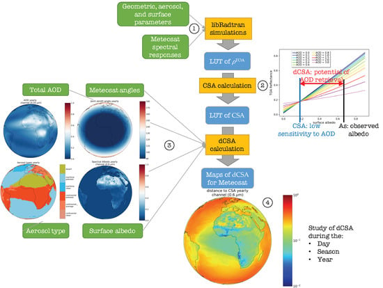
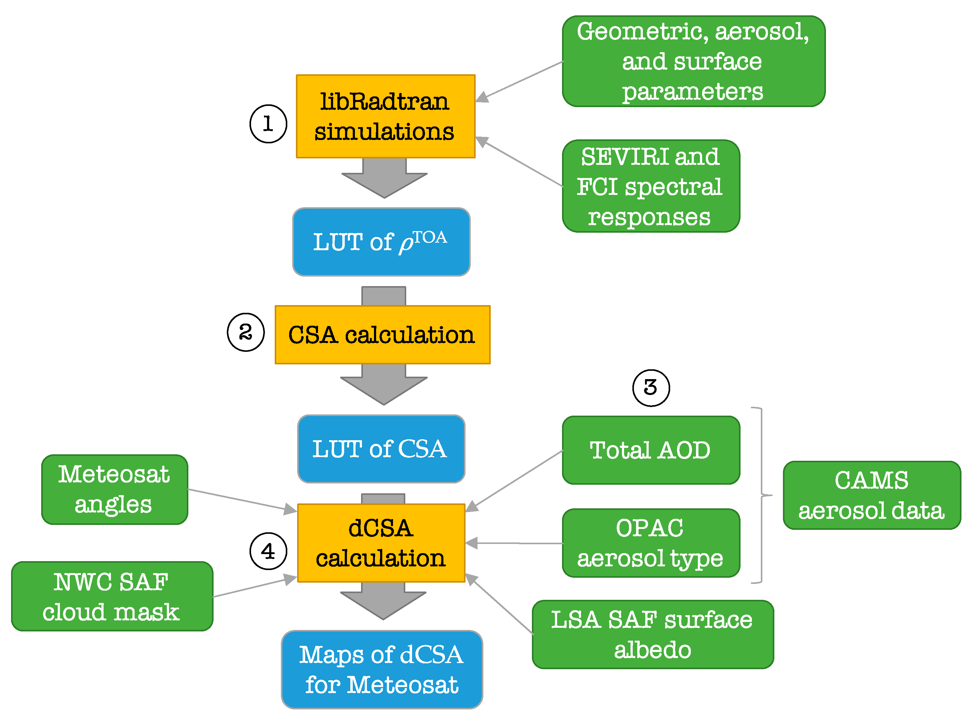
2.1. Overview
2.2. Look-up Table of TOA Reflectance
2.3. Look-Up Table of CSA
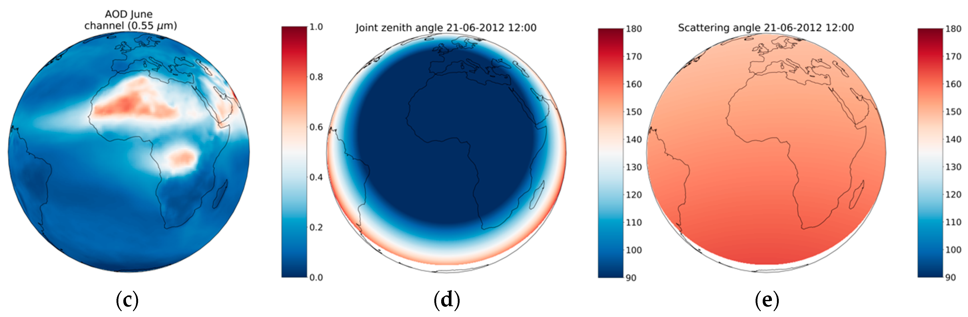
2.4. Input Data to Compute Maps of dCSA for Meteosat
2.4.1. Geometry
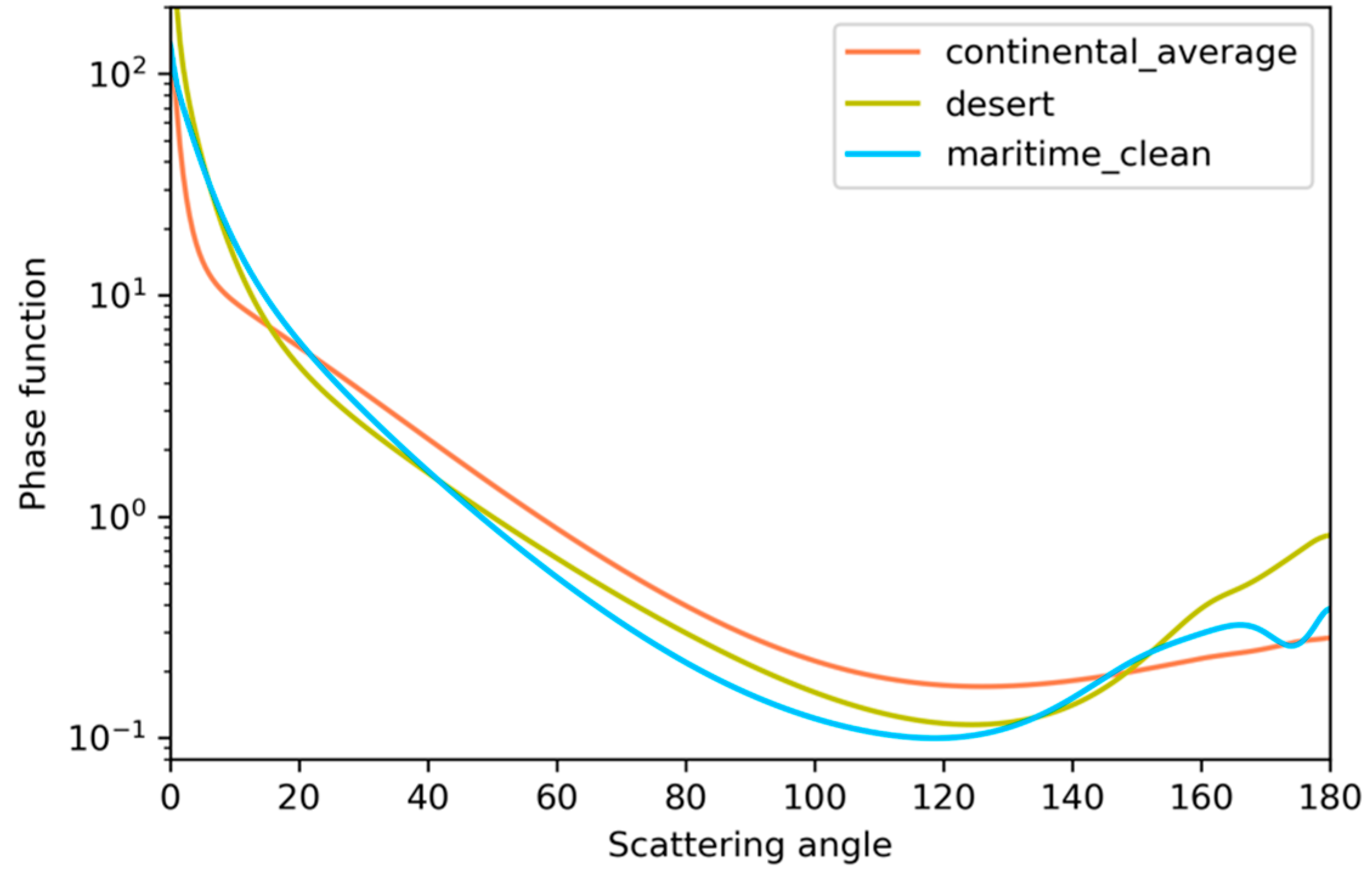
2.4.2. Aerosol Properties
2.4.3. Surface Albedo
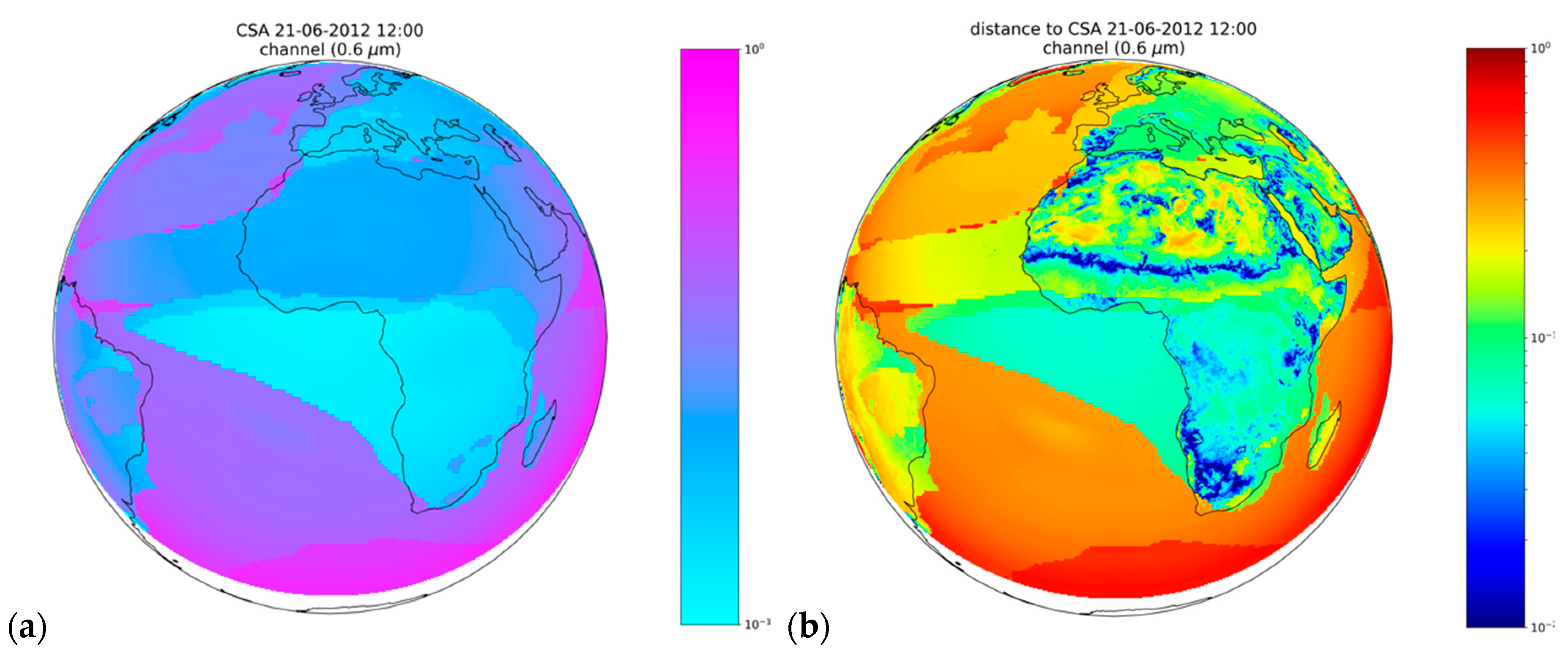
2.5. Calculation of Maps of dCSA for Meteosat
3. Results
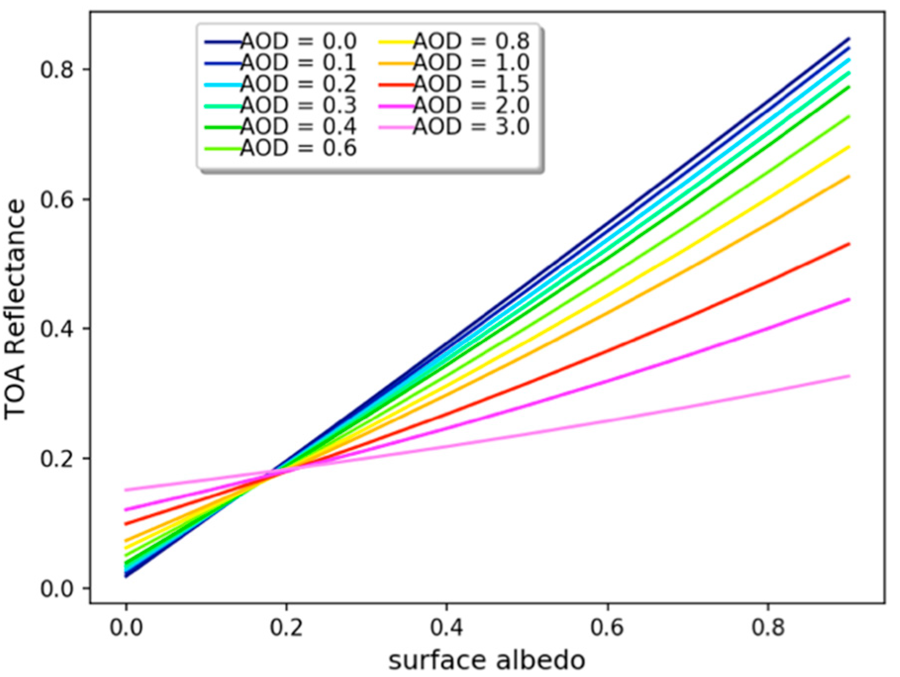
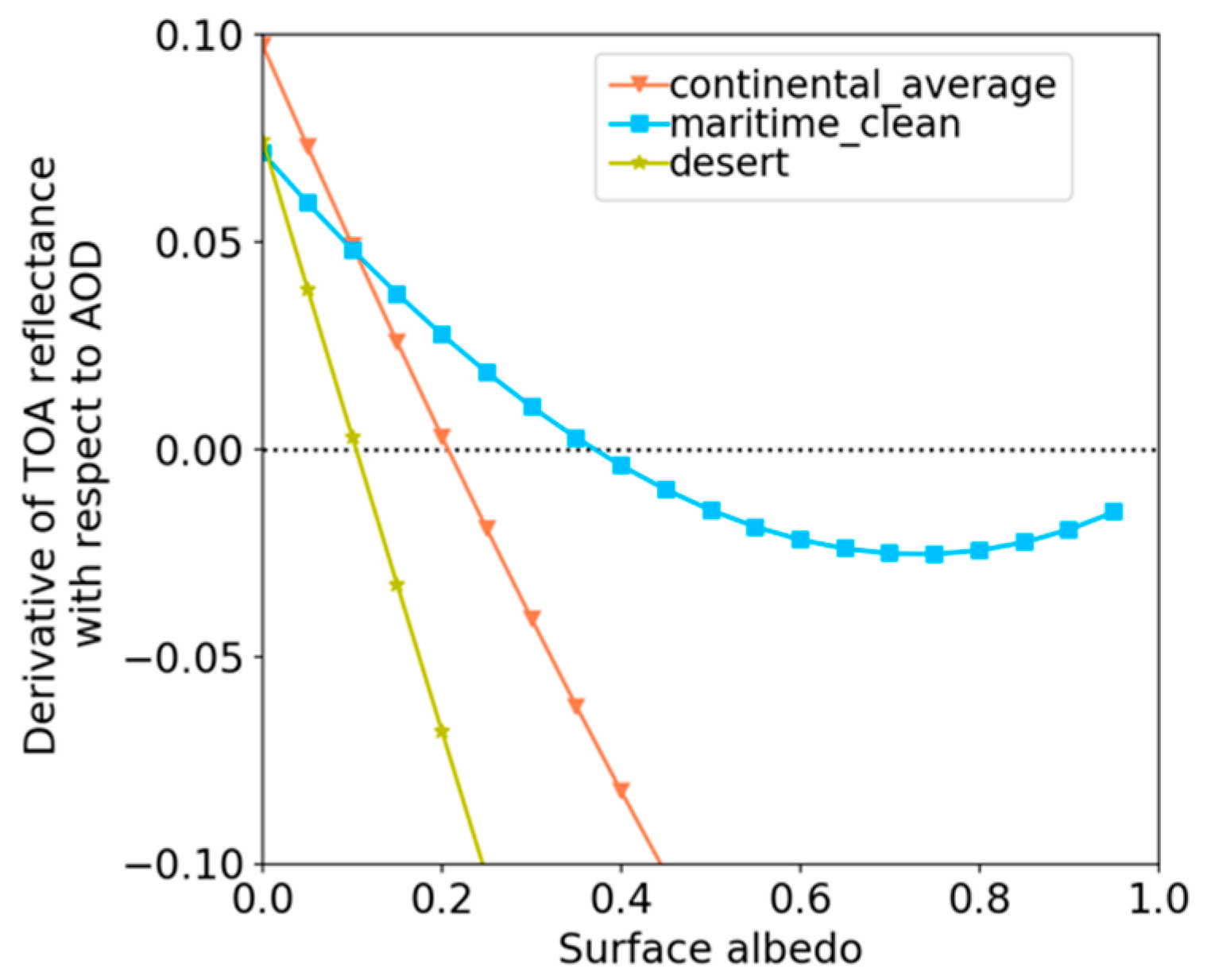
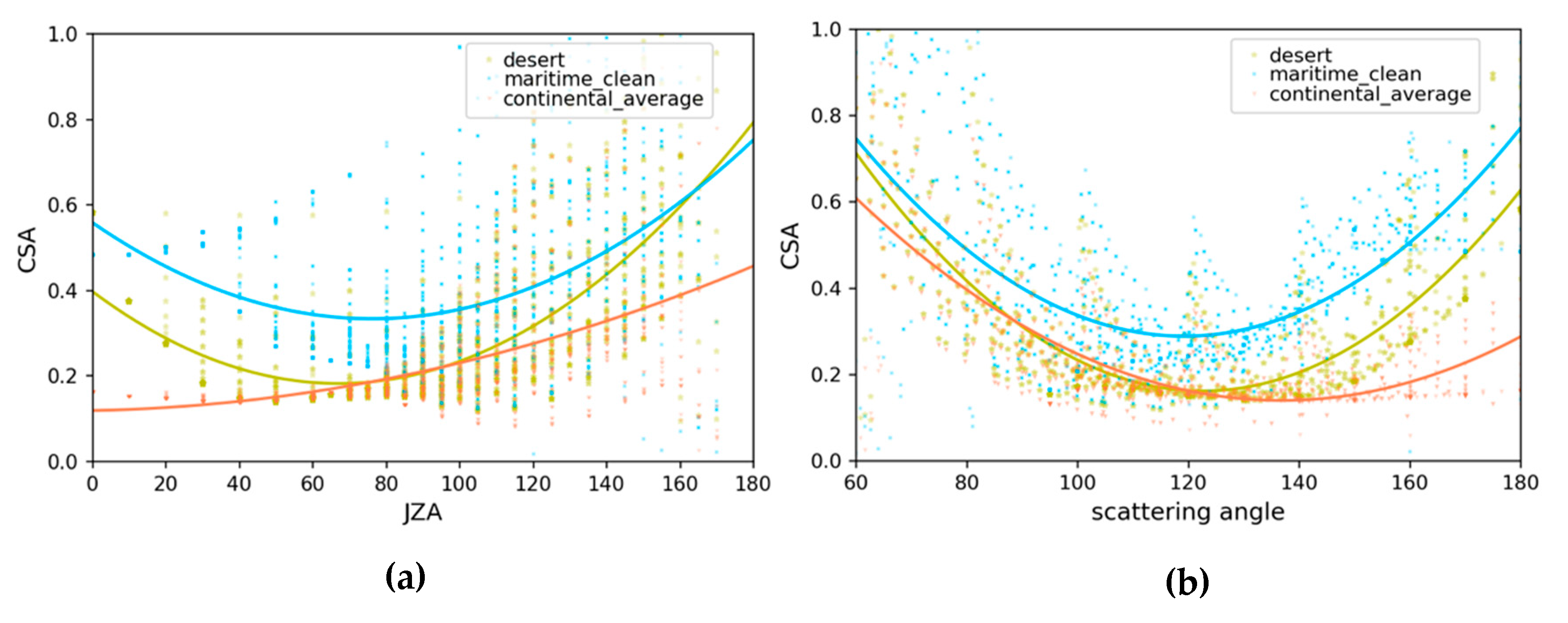
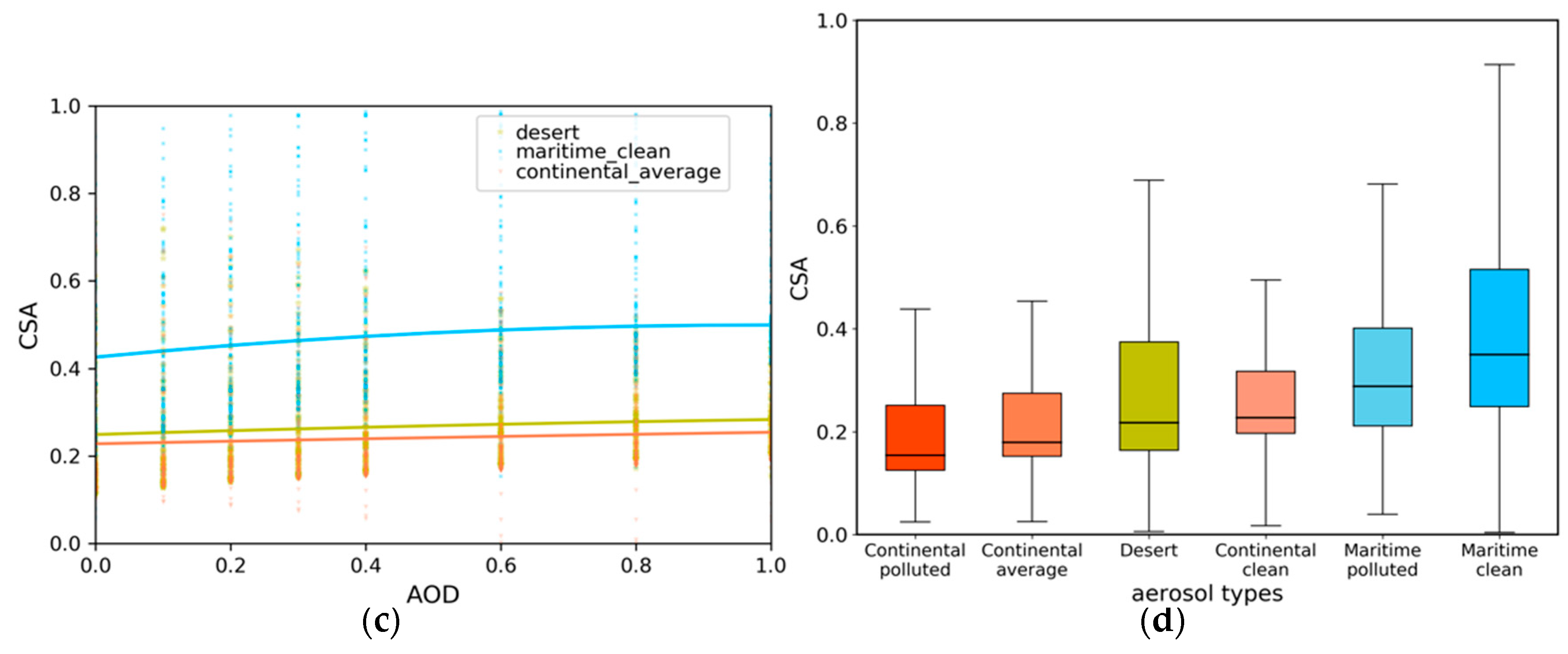
3.1. Dependence of CSA on the Remote Sensing Parameters
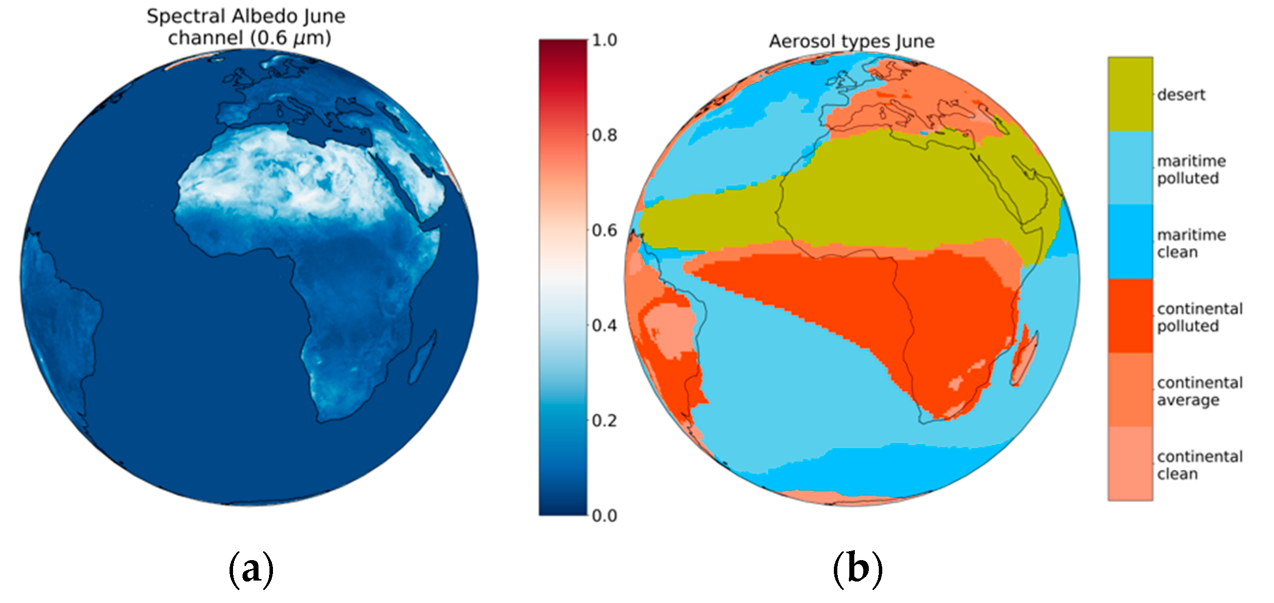
3.2. Calculation of the Map of dCSA for One Meteosat Image
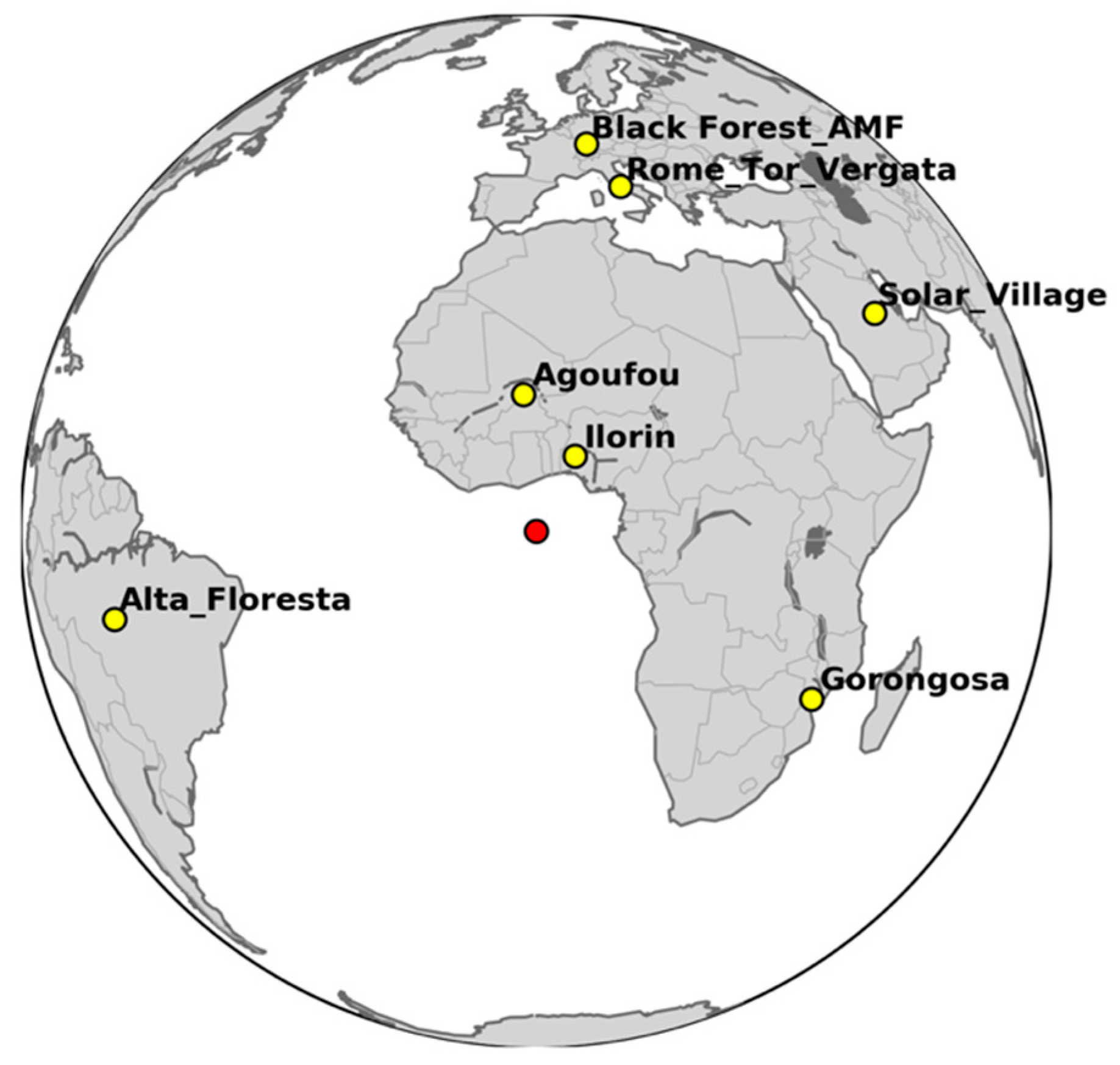
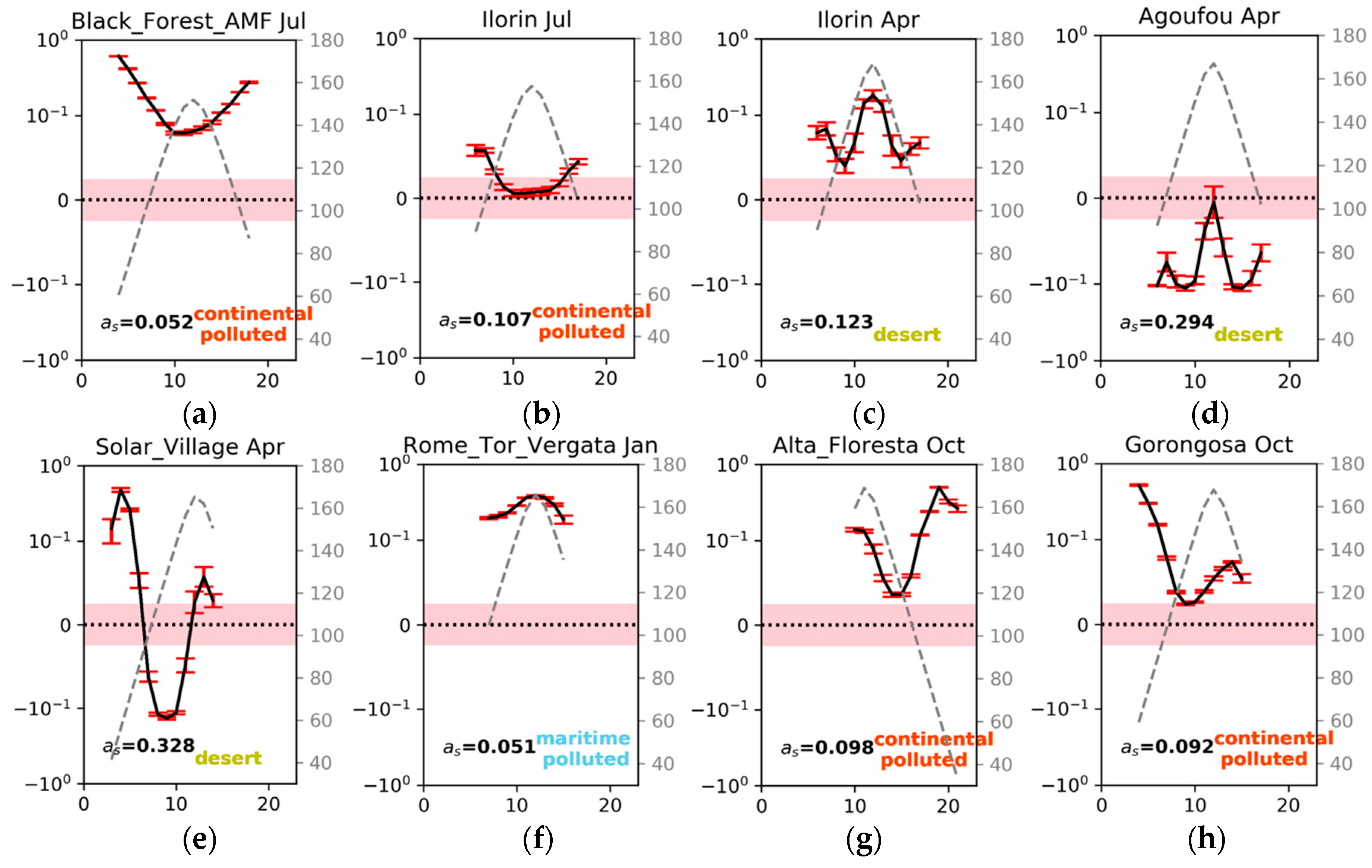
3.3. Diurnal Study
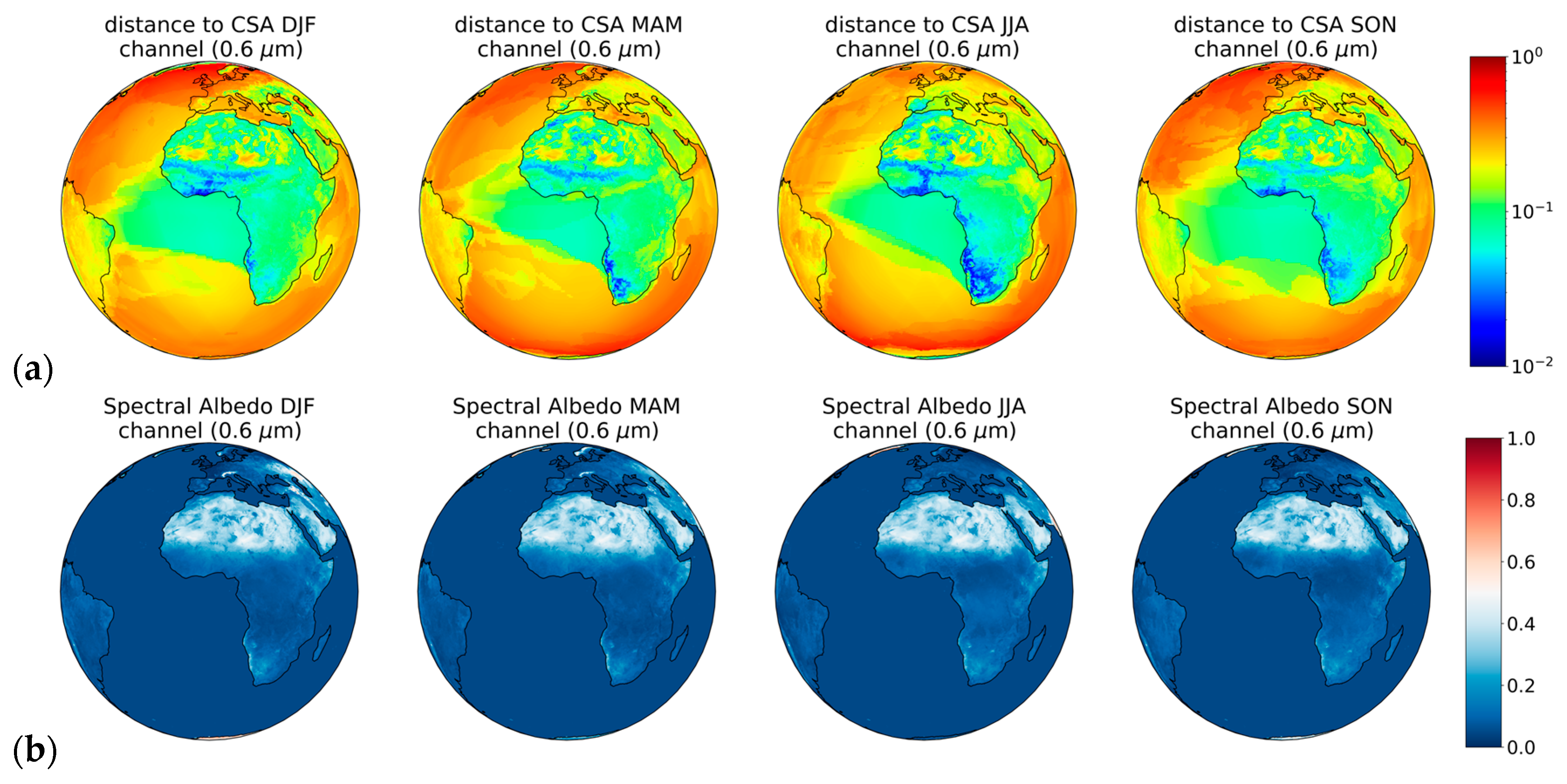
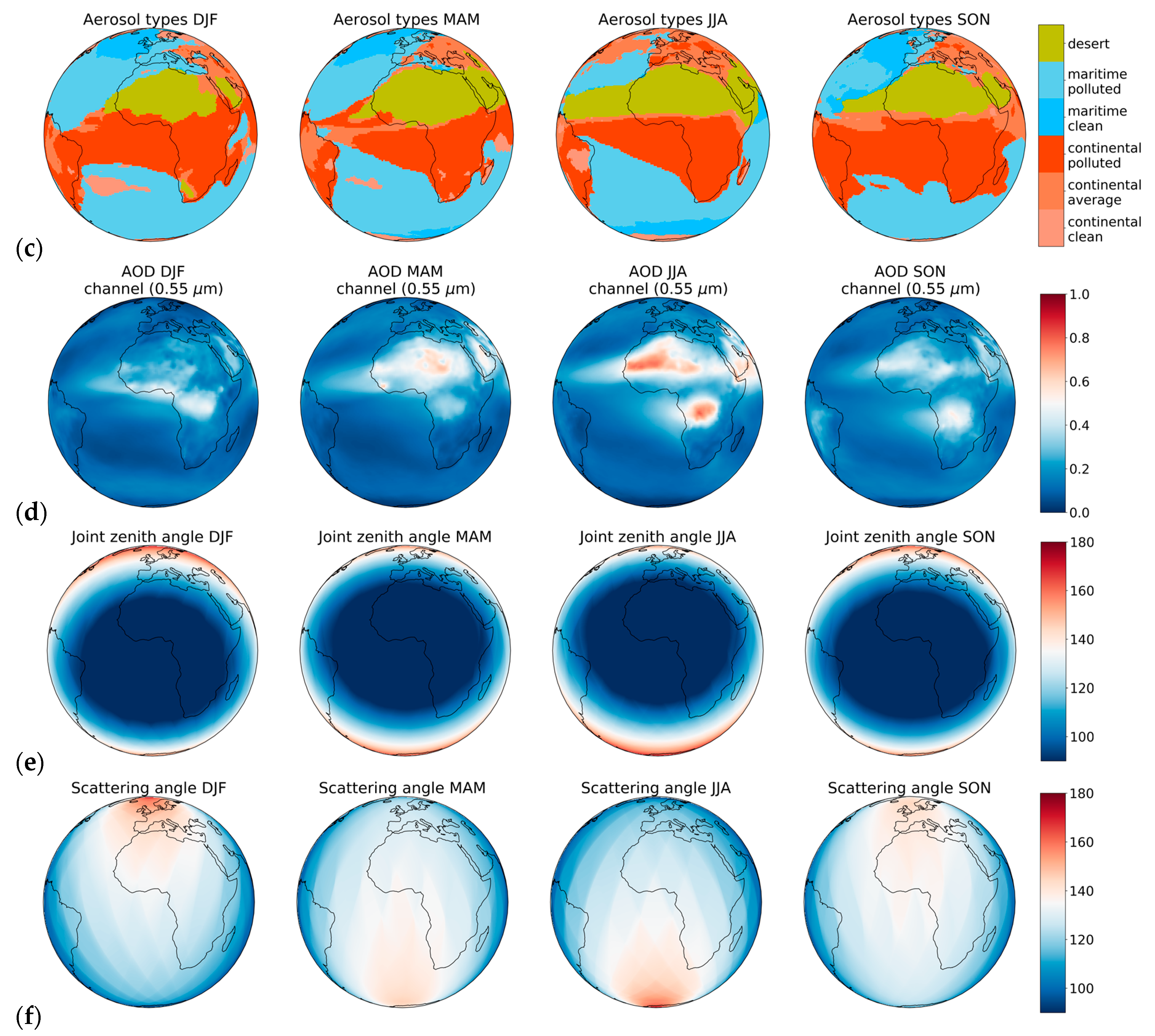
3.4. Seasonal Study
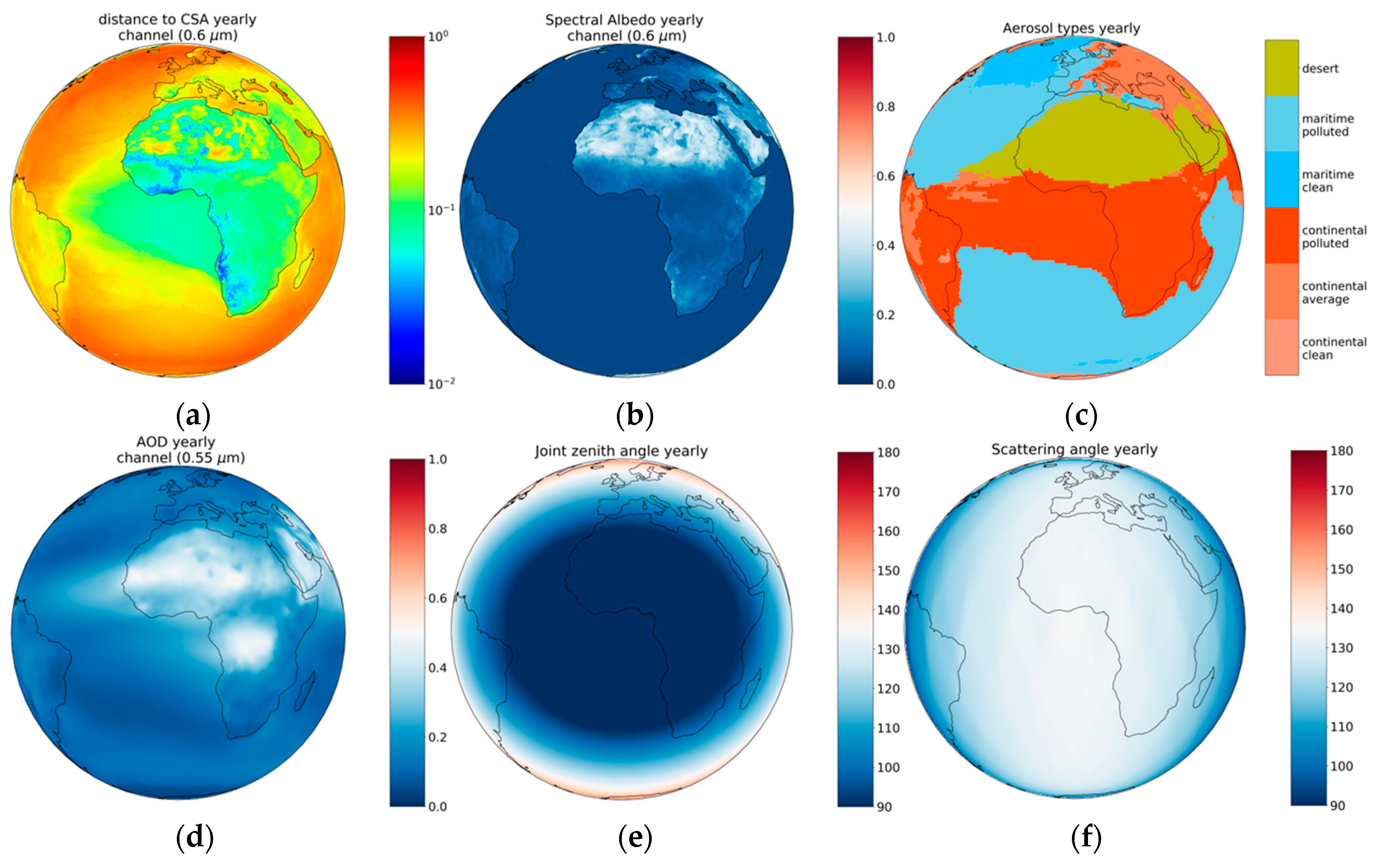
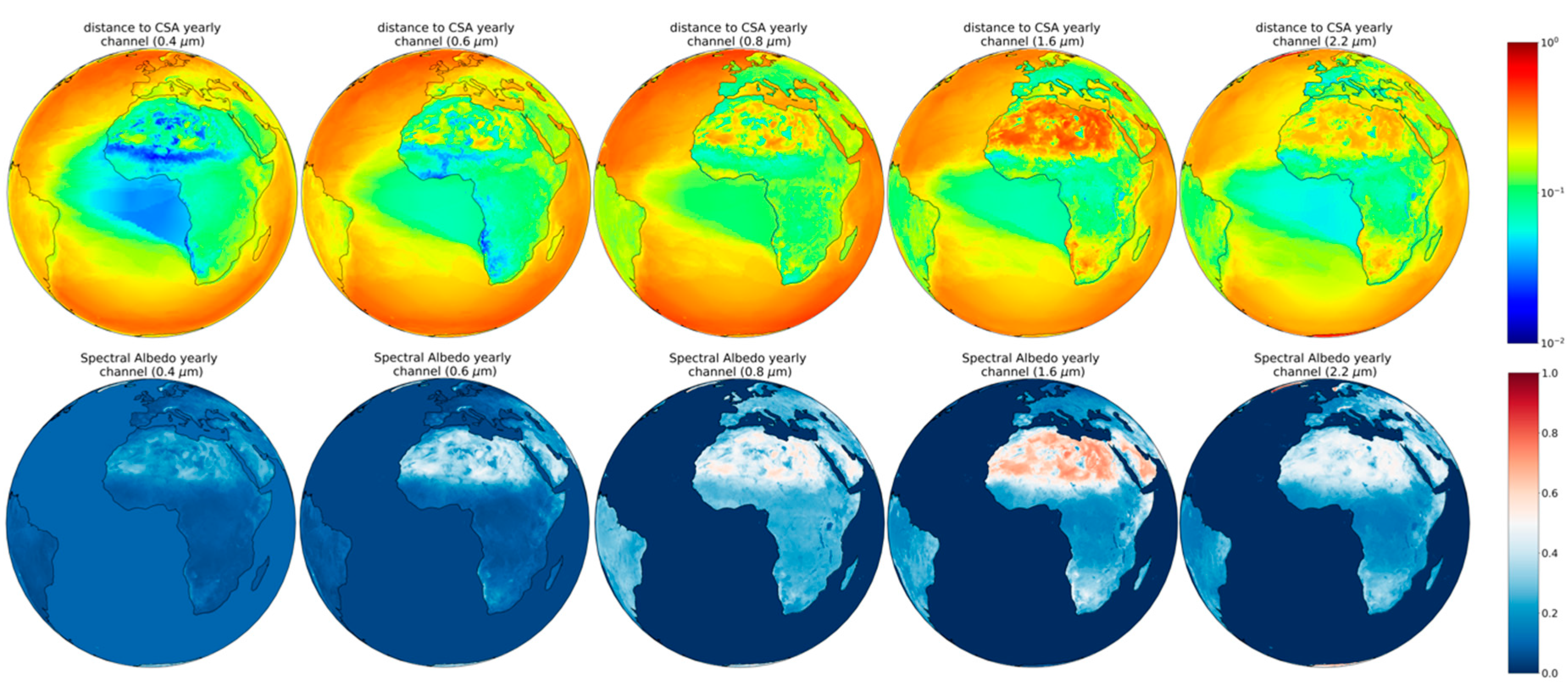
3.5. Yearly Study
3.5.1. Wavelength Dependence
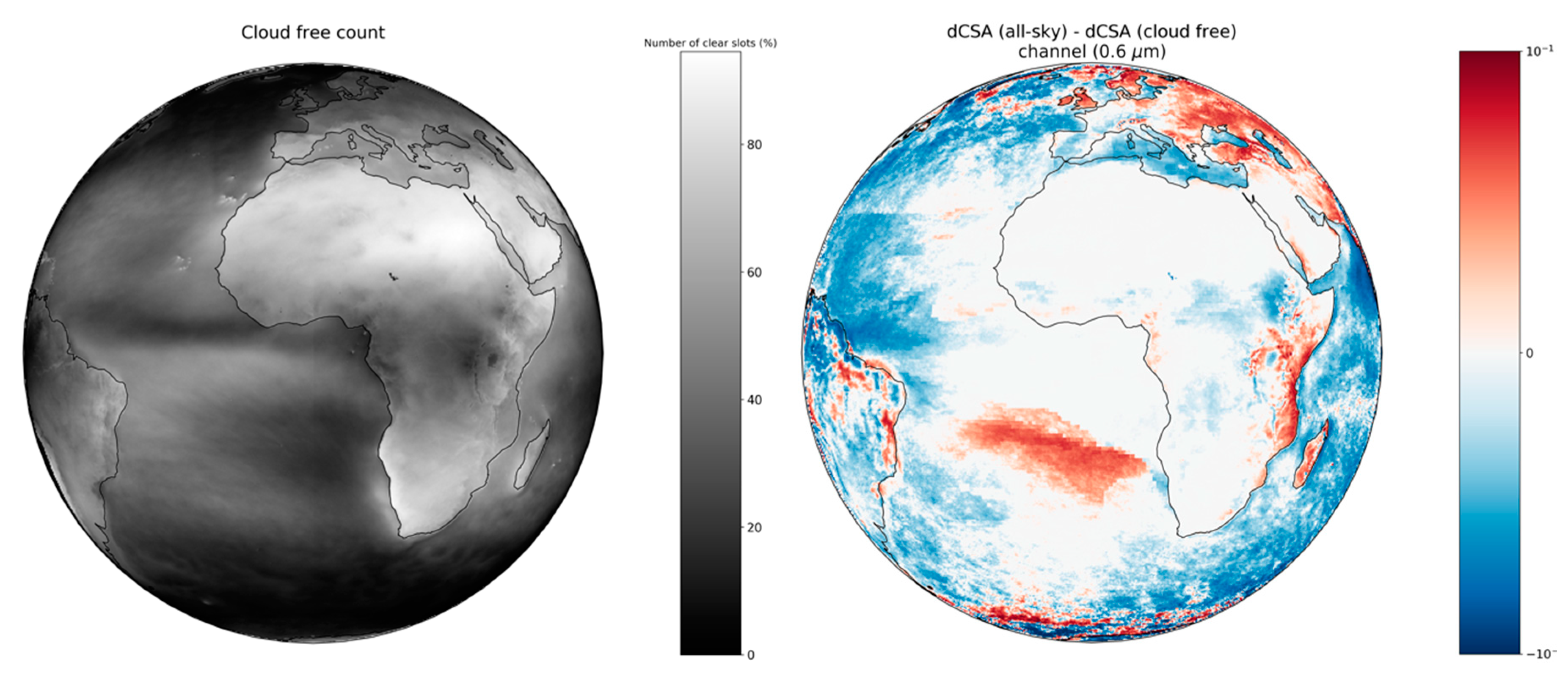
3.5.2. Impact of Cloudiness
4. Discussion
4.1. dCSA and Sensitivity to Aerosols
4.1.1. Geometric and Temporal Information
4.1.2. Spatial Information
4.1.3. Spectral Information
4.2. Limitations
4.3. Implications to Remote Sensing and Future Directions
5. Conclusions
Author Contributions
Funding
Acknowledgments
Conflicts of Interest
Appendix A

| continental_average | desert | maritime_clean | |
|---|---|---|---|
| 0.492 | 0.543 | 0.660 | |
| 0.526 | 0.812 | 1.137 | |
| 0.409 | 0.954 | 1.308 | |
| −0.540 | −0.858 | −0.586 | |
| −0.792 | −0.865 | −0.994 | |
| −0.747 | −0.512 | −0.969 | |
| −0.609 | −0.729 | −0.789 | |
| 1.709 | 2.678 | 2.665 | |
| R-value | 0.973 | 0.908 | 0.915 |
| Bias | 0.000 | 0.000 | 0.000 |
| RMSE | 0.013 | 0.048 | 0.061 |
References
- Boucher, O.; Randall, D.; Artaxo, P.; Bretherton, C.; Feingold, G.; Forster, P.; Kerminen, V.-M.; Kondo, Y.; Liao, H.; Lohmann, U.; et al. Clouds and Aerosols. In Climate Change 2013: The Physical Science Basis. Contribution of Working Group I to the Fifth Assessment Report of the Intergovernmental Panel on Climate Change; Stocker, T.F., Qin, D., Plattner, G.-K., Tignor, M., Allen, S.K., Boschung, J., Nauels, A., Xia, Y., Bex, V., Midgley, P.M., Eds.; Cambridge University Press: Cambridge, UK; New York, NY, USA, 2013. [Google Scholar]
- Kaufman, Y.; Tanré, D.; Boucher, O. A satellite view of aerosols in the climate system. Nature 2002, 419, 215–223. [Google Scholar] [CrossRef] [PubMed]
- King, M.D.; Dubovik, O. Determination of aerosol optical properties from inverse methods. In Aerosol Remote Sensing; Lenoble, J., Remer, L., Tanré, D., Eds.; Springer: Berlin/Heidelberg, Germany, 2013; pp. 13–51. [Google Scholar]
- Laszlo, I.; Ciren, P.; Liu, H.; Kondragunta, S.; Tarpley, J.D.; Goldberg, M.D. Remote sensing of aerosol and radiation from geostationary satellites. Adv. Space Res. 2008, 41, 1882–1893. [Google Scholar] [CrossRef]
- Timmermans, R.M.; Schaap, M.; Builtjes, P.; Elbern, H.; Siddans, R.; Tjemkes, S.; Vautard, R. An Observing System Simulation Experiment (OSSE) for Aerosol Optical Depth from Satellites. J. Atmos. Oceanic Technol. 2009, 26, 2673–2682. [Google Scholar] [CrossRef]
- Castellanos, P.; Da Silva, A.M.; Darmenov, A.S.; Buchard, V.; Govindaraju, R.C.; Ciren, P.; Kondragunta, S. A Geostationary Instrument Simulator for Aerosol Observing System Simulation Experiments. Atmosphere 2019, 10, 2. [Google Scholar] [CrossRef]
- Goto, D.; Kikuchi, M.; Suzuki, K.; Hayasaki, M.; Yoshida, M.; Nagao, T.M.; Choi, M.; Kim, J.; Sugimoto, N.; Shimizu, A.; et al. Aerosol model evaluation using two geostationary satellites over East Asia in May 2016. Atmos. Res. 2019, 217, 93–113. [Google Scholar] [CrossRef]
- Schmetz, J.; Pili, P.; Tjemkes, S.; Just, D.; Kerkmann, J.; Rota, S.; Ratier, A. An Introduction to Meteosat Second Generation (MSG). Bull. Am. Meteorol. Soc. 2002, 83, 977–992. [Google Scholar] [CrossRef]
- Schmit, T.J.; Gunshor, M.M.; Menzel, W.P.; Gurka, J.J.; Li, J.; Bachmeier, A.S. Introducing the next generation Advanced Baseline Imager on GOES-R. Bull. Am. Meteorol. Soc. 2005, 86, 1079–1096. [Google Scholar] [CrossRef]
- Bessho, K.; Date, K.; Hayashi, M.; Ikeda, A.; Imai, T.; Inoue, H.; Kumagai, Y.; Miyakawa, T.; Murata, H.; Ohno, T.; et al. An introduction to Himawari-8/9 - Japan’s new-generation geostationary meteorological satellites. J. Meteorol. Soc. Jpn. Ser. II 2016, 94, 151–183. [Google Scholar] [CrossRef]
- Klaes, K.D. An update on EUMETSAT programmes and plans. In Earth Observing Systems XXIII; International Society for Optics and Photonics: San Diego, CA, USA, 2018; Volume 10764. [Google Scholar]
- Descheemaecker, M.; Plu, M.; Marécal, V.; Claeyman, M.; Olivier, F.; Aoun, Y.; Blanc, P.; Wald, L.; Guth, J.; Sič, B.; et al. Monitoring aerosols over Europe: An assessment of the potential benefit of assimilating the VIS04 measurements from the future MTG/FCI geostationary imager. Atmos. Meas. Technol. 2019, 12, 1251–1275. [Google Scholar] [CrossRef]
- Aoun, Y. Évaluation de la sensibilité de l’instrument FCI à bord du nouveau satellite Meteosat Troisième Génération imageur (MTG-I) aux variations de la quantité d’aérosols d’origine désertique dans l’atmosphère. Ph.D. Thesis, MINES ParisTech, PSL - Research University, Sophia Antipolis, France, 2016. [Google Scholar]
- Knapp, K.R.; Vonder Haar, T.H.; Kaufman, Y.J. Aerosol optical depth retrieval from GOES-8: Uncertainty study and retrieval validation over South America. J. Geophys. Res. 2002, 107, AAC-2. [Google Scholar] [CrossRef]
- Prados, A.I.; Kondragunta, S.; Ciren, P.; Knapp, K.R. GOES Aerosol/Smoke Product (GASP) over North America: Comparisons to AERONET and MODIS observations. J. Geophys. Res. 2007, 112, D15201. [Google Scholar] [CrossRef]
- Carrer, D.; Roujean, J.-L.; Hautecoeur, O.; Elias, T. Daily estimates of aerosol optical thickness over land surface based on a directional and temporal analysis of SEVIRI MSG visible observations. J. Geophys. Res. Atmos. 2010, 115, D10208. [Google Scholar] [CrossRef]
- Govaerts, Y.M.; Wagner, S.; Lattanzio, A.; Watts, P. Joint retrieval of surface reflectance and aerosol optical depth from MSG/SEVIRI observations with an optimal estimation approach: 1. Theory. J. Geophys. Res. 2010, 115, D0220. [Google Scholar] [CrossRef]
- Wagner, S.C.; Govaerts, Y.M.; Lattanzio, A. Joint retrieval of surface reflectance and aerosol optical depth from MSG/SEVIRI observations with an optimal estimation approach: 2. Implementation and evaluation. J. Geophys. Res. 2010, 115, D02204. [Google Scholar] [CrossRef]
- Zhang, H.; Lyapustin, A.; Wang, Y.; Kondragunta, S.; Laszlo, I.; Ciren, P.; Hoff, R.M. A multi-angle aerosol optical depth retrieval algorithm for geostationary satellite data over the United States. Atmos. Chem. Phys. 2011, 11, 11977–11991. [Google Scholar] [CrossRef]
- Carrer, D.; Ceamanos, X.; Six, B.; Roujean, J.-L. AERUS-GEO: A newly available satellite-derived aerosol optical depth product over Europe and Africa. Geophys. Res. Lett. 2014, 41, 7731–7738. [Google Scholar] [CrossRef]
- GOES-R Advanced Baseline Imager (ABI) Algorithm Theoretical Basis Document For Suspended Matter/Aerosol Optical Depth and Aerosol Size Parameter; Version 4.2; NOAA Nesdis Center for Satellite Applications and Research: Grand Forks, ND, USA, 2018.
- Yoshida, M.; Kikuchi, M.; Nagao, T.M.; Murakami, H.; Nomaki, T.; Higurashi, A. Common retrieval of aerosol properties for imaging satellite sensors. J. Meteor. Soc. Jpn. 2018, 96B, 193–209. [Google Scholar] [CrossRef]
- Shi, S.; Cheng, T.; Gu, X.; Letu, H.; Guo, H.; Chen, H.; Wu, Y. Synergistic Retrieval of Multi-temporal Aerosol Optical Depth over North China Plain Using Geostationary Satellite Data of Himawari-8. J. Geophys. Res. Atmos. 2018, 123, 5525–5537. [Google Scholar] [CrossRef]
- Govaerts, Y.; Luffarelli, M. Joint retrieval of surface reflectance and aerosol properties with continuous variation of the state variables in the solution space—Part 1: Theoretical concept. Atmos. Meas. Tech. 2018, 11, 6589–6603. [Google Scholar] [CrossRef]
- Luffarelli, M.; Govaerts, Y. Joint retrieval of surface reflectance and aerosol properties with continuous variation of the state variables in the solution space – Part 2: Application to geostationary and polar-orbiting satellite observations. Atmos. Meas. Tech. 2019, 12, 791–809. [Google Scholar] [CrossRef]
- Gupta, P.; Levy, R.C.; Mattoo, S.; Remer, L.A.; Holz, R.E.; Heidinger, A.K. Retrieval of aerosols over Asia from the Advanced Himawari Imager: Expansion of temporal coverage of the global Dark Target aerosol product. Atmos. Meas. Tech. Discuss. 2019. [Google Scholar] [CrossRef]
- Lenoble, J.; Mishchenko, M.I.; Herman, M. Absorption and Scattering by Molecules and Particles. In Aerosol Remote Sensing; Lenoble, J., Remer, L., Tanré, D., Eds.; Springer: Berlin/Heidelberg, Germany, 2013; pp. 13–51. [Google Scholar]
- Fraser, R.; Kaufman, Y. The Relative Importance of Aerosol Scattering and Absorption in Remote Sensing. IEEE Trans. Geosci. Remote Sens. 1985, GE-23, 625–633. [Google Scholar]
- De Almeida Castanho, A.D.; Vanderlei Martins, J.; Artaxo, P. MODIS Aerosol Optical Depth Retrievals with high spatial resolution over an Urban Area using the Critical Reflectance. J. Geophys. Res. 2008, 113, D02201. [Google Scholar] [CrossRef]
- Zhu, L.; Martins, J.V.; Remer, L.A. Biomass burning aerosol absorption measurements with MODIS using the critical reflectance method. J. Geophys. Res. 2011, 116, D07202. [Google Scholar] [CrossRef]
- Wells, K.C.; Martins, J.V.; Remer, L.A.; Kreidenweis, S.M.; Stephens, G.L. Critical reflectance derived from MODIS: Application for the retrieval of aerosol absorption over desert regions. J. Geophys. Res. 2012, 117, D03202. [Google Scholar] [CrossRef]
- Seidel, F.C.; Popp, C. Critical surface albedo and its implications to aerosol remote sensing. Atmos. Meas. Tech. 2012, 5, 1653–1665. [Google Scholar] [CrossRef]
- Boehmler, J.M.; Loría-Salazar, S.M.; Stevens, C.; Long, J.D.; Watts, A.C.; Holmes, H.A.; Barnard, J.C.; Arnott, W.P. Development of a Multispectral Albedometer and Deployment on an Unmanned Aircraft for Evaluating Satellite Retrieved Surface Reflectance over Nevada’s Black Rock Desert. Sensors 2018, 18, 3504. [Google Scholar] [CrossRef]
- Cochrane, S.P.; Schmidt, K.S.; Chen, H.; Pilewskie, P.; Kittelman, S.; Redemann, J.; LeBlanc, S.; Pistone, K.; Kacenelenbogen, M.; Segal Rozenhaimer, M.; et al. Above-Cloud Aerosol Radiative Effects based on ORACLES 2016 and ORACLES 2017 Aircraft Experiments. Atmos. Meas. Tech. Discuss. 2019. [Google Scholar] [CrossRef]
- Zhang, Q.; Shia, R.-L.; Sander, S.P.; Yung, Y.L. XCO2 retrieval error over deserts near critical surface albedo. Earth Space Sci. 2016, 3, 36–45. [Google Scholar] [CrossRef]
- Mayer, B.; Kylling, A. Technical note: The libRadtran software package for radiative transfer calculations - description and examples of use. Atmos. Chem. Phys. 2005, 5, 1855–1877. [Google Scholar] [CrossRef]
- Emde, C.; Buras-Schnell, R.; Kylling, A.; Mayer, B.; Gasteiger, J.; Hamann, U.; Kylling, J.; Richter, B.; Pause, C.; Dowling, T.; et al. The libRadtran software package for radiative transfer calculations (version 2.0.1). Geosci. Model Dev. 2016, 9, 1647–1672. [Google Scholar] [CrossRef]
- Anderson, G.P.; Clough, S.A.; Kneizys, F.X.; Chetwynd, J.H.; Shettle, E.P. AFGL Atmospheric Constituent Profiles (0–120 km); AFGL-TR-86-0110; Air Force Geophysics Laboratory, Hanscom Air Force Base: Bedford, MA, USA, 1986; 43p. [Google Scholar]
- Hess, M.; Koepke, P.; Schult, I. Optical Properties of Aerosols and Clouds: The Software Package OPAC. Bull. Am. Meteorol. Soc. 1998, 79, 831–844. [Google Scholar] [CrossRef]
- Gasteiger, J.; Wiegner, M. MOPSMAP v1.0: A versatile tool for the modeling of aerosol optical properties. Geosci. Model Dev. 2018, 11, 2739–2762. [Google Scholar] [CrossRef]
- Lefèvre, M.; Oumbe, A.; Blanc, P.; Espinar, B.; Gschwind, B.; Qu, Z.; Wald, L.; Schroedter-Homscheidt, M.; Hoyer-Klick, C.; Arola, A.; et al. McClear: A new model estimating downwelling solar radiation at ground level in clear-sky conditions. Atmos. Meas. Tech. 2013, 6, 2403–2418. [Google Scholar] [CrossRef]
- Geiger, B.; Carrer, D.; Franchisteguy, L.; Roujean, J.-L.; Meurey, C. Land Surface Albedo Derived on a Daily Basis From Meteosat Second Generation Observations. IEEE Trans. Geosci. Remote Sens. 2008, 46, 3841–3856. [Google Scholar] [CrossRef]
- Carrer, D.; Roujean, J.-L.; Meurey, C. Comparing operational MSG/SEVIRI land surface albedo products from Land SAF with ground measurements and MODIS. IEEE Trans. Geosci. Remote Sens. 2010, 48, 1714–1728. [Google Scholar] [CrossRef]
- Samain, O.; Geiger, B.; Roujean, J.-L. Spectral normalization and fusion of optical sensors for the retrieval of BRDF and albedo: Application to VEGETATION, MODIS, and MERIS data sets. IEEE Trans. Geosci. Remote Sens. 2006, 44, 3166–3179. [Google Scholar] [CrossRef]
- Feng, Y.; Liu, Q.; Ying, Q.; Liang, S. Estimation of the ocean water albedo from remote sensing and meteorological reanalysis data. IEEE Trans. Geosci. Remote Sens. 2016, 54, 850–868. [Google Scholar] [CrossRef]
- Proud, S.R.; Fensholt, R.; Rasmussen, M.O.; Sandholt, I. A comparison of the effectiveness of 6S and SMAC in correcting for atmospheric interference of Meteosat Second Generation images. J. Geophys. Res. 2010. [Google Scholar] [CrossRef]
- Jones, H.M.; Crosier, J.; Russel, A.; Flynn, M.J.; Irwin, M.; Choularton, T.W.; Coe, H.; McFiggans, G. In situ aerosol measurements taken during the 2007 COPS field campaign at the Hornisgrinde ground site. Q. J. R. Meteorol. Soc. 2011, 137, 252–266. [Google Scholar] [CrossRef]
- Dramé, M.S.; Ceamanos, X.; Roujean, J.L.; Boone, A.; Lafore, J.P.; Carrer, D.; Geoffroy, O. On the Importance of Aerosol Composition for Estimating Incoming Solar Radiation: Focus on the Western African Stations of Dakar and Niamey during the Dry Season. Atmosphere 2015, 6, 1608–1632. [Google Scholar] [CrossRef]
- Adesina, A.J.; Kumar, K.R.; Sivakumar, V. Variability in aerosol optical properties and radiative forcing over Gorongosa (18.97°S, 34.35°E) in Mozambique. Meteorol. Atmos. Phys. 2015, 127, 217–228. [Google Scholar] [CrossRef]
- Bozzo, A.; Remy, S.; Benedetti, A.; Flemming, J.; Bechtold, P.; Rodwell, M.J.; Morcrette, J.-J. Implementation of a CAMS-Based Aerosol Climatology in the IFS; Technical Memorandum, Research Department, ECMWF: Reading, England, 2017. [Google Scholar]
- Ba, M.B.; Nicholson, S.E.; Frouin, R. Satellite-derived surface radiation budget over the African continent. Part II: Climatologies of the various components. J. Clim. 2001, 14, 60–76. [Google Scholar] [CrossRef]
- Menut, L.; Flamant, C.; Turquety, S.; Deroubaix, A.; Chazette, P.; Meynadier, R. Impact of biomass burning on pollutant surface concentrations in megacities of the Gulf of Guinea. Atmos. Chem. Phys. 2018, 18, 2687–2707. [Google Scholar] [CrossRef]
- Derrien, M.; Le Gleau, H. MSG/SEVIRI cloud mask and type from SAFNWC. Int. J. Remote Sens. 2005, 26, 4707–4732. [Google Scholar] [CrossRef]
- Zieger, P.; Fierz-Schmidhauser, R.; Weingartner, E.; Baltensperger, U. Effects of relative humidity on aerosol light scattering: Results from different European sites. Atmos. Chem. Phys. 2013, 13, 10609–10631. [Google Scholar] [CrossRef]
- Moparthy, S.; Carrer, D.; Ceamanos, X. Can we detect the browness or greenness of the Congo rainforest using satellite-derived surface albedo? A study on the role of aerosol uncertaintites. Suistainability 2019, 11, 1410. [Google Scholar] [CrossRef]
- Witek, M.L.; Garay, M.J.; Diner, D.J.; Bull, M.A.; Seidel, F.C. New approach to the retrieval of AOD and its uncertainty from MISR observations over dark water. Atmos. Meas. Tech. 2018, 11, 429–439. [Google Scholar] [CrossRef]
- Sayer, A.M.; Govaerts, Y.; Kolmonen, P.; Lipponen, A.; Luffarelli, M.; Mielonen, T.; Patadia, F.; Popp, T.; Povey, A.C.; Stebel, K.; et al. A review and framework for the evaluation of pixel-level uncertainty estimates in satellite aerosol remote sensing. Atmos. Meas. Tech. Discuss. 2019. [Google Scholar] [CrossRef]
- Anderson, T.L.; Charlson, R.J.; Winker, D.M.; Ogren, J.A.; Holmén, K. Mesoscale Variations of Tropospheric Aerosols. J. Atmos. Sci. 2003, 60, 119–136. [Google Scholar] [CrossRef]


| Geometry | Aerosols | Surface | Spectral | ||||
|---|---|---|---|---|---|---|---|
| SZA (°) | VZA (°) | RAA (°) | AOD 550 nm | Aerosol type | Albedo | Channel | Wavelength (µm) |
| 0:5:85 | 0:5:85 | 0:20:180 | 0, 0.1, 0.2, 0.3, 0.4, 0.6, 0.8, 1.0, 1.5, 2.0, 3.0 | continental_clean continental_average continental_polluted desert maritime_clean maritime_polluted | 0:0.05:1 | VIS04 1 VIS06 VIS08 IR016 IR022 1 | 0.44 0.63 0.81 1.64 2.25 |
| Aerosol type | VIS06 | IR016 | ||
|---|---|---|---|---|
| SSA | g | SSA | g | |
| continental_clean | 0.94 | 0.68 | 0.85 | 0.68 |
| continental_average | 0.89 | 0.66 | 0.77 | 0.66 |
| continental_polluted | 0.84 | 0.65 | 0.68 | 0.63 |
| desert | 0.92 | 0.7 | 0.94 | 0.69 |
| maritime_clean | 0.98 | 0.75 | 0.98 | 0.79 |
| maritime_polluted | 0.96 | 0.74 | 0.96 | 0.78 |
| Channel | Surface Albedo |
|---|---|
| VIS04 | 0.1 |
| VIS06 | 0.05 |
| VIS08 | 0.01 |
| IR016 | 0 |
| IR022 | 0 |
© 2019 by the authors. Licensee MDPI, Basel, Switzerland. This article is an open access article distributed under the terms and conditions of the Creative Commons Attribution (CC BY) license (http://creativecommons.org/licenses/by/4.0/).
Share and Cite
Ceamanos, X.; Moparthy, S.; Carrer, D.; Seidel, F.C. Assessing the Potential of Geostationary Satellites for Aerosol Remote Sensing Based on Critical Surface Albedo. Remote Sens. 2019, 11, 2958. https://doi.org/10.3390/rs11242958
Ceamanos X, Moparthy S, Carrer D, Seidel FC. Assessing the Potential of Geostationary Satellites for Aerosol Remote Sensing Based on Critical Surface Albedo. Remote Sensing. 2019; 11(24):2958. https://doi.org/10.3390/rs11242958
Chicago/Turabian StyleCeamanos, Xavier, Suman Moparthy, Dominique Carrer, and Felix C. Seidel. 2019. "Assessing the Potential of Geostationary Satellites for Aerosol Remote Sensing Based on Critical Surface Albedo" Remote Sensing 11, no. 24: 2958. https://doi.org/10.3390/rs11242958
APA StyleCeamanos, X., Moparthy, S., Carrer, D., & Seidel, F. C. (2019). Assessing the Potential of Geostationary Satellites for Aerosol Remote Sensing Based on Critical Surface Albedo. Remote Sensing, 11(24), 2958. https://doi.org/10.3390/rs11242958