Abstract
Nowadays, GF-1 (GF is the acronym for GaoFen which means high-resolution in Chinese) remote sensing images are widely utilized in agriculture because of their high spatio-temporal resolution and free availability. However, due to the transferrable rationale of optical satellites, the GF-1 remote sensing images are inevitably impacted by clouds, which leads to a lack of ground object’s information of crop areas and adds noises to research datasets. Therefore, it is crucial to efficiently detect the cloud pixel of GF-1 imagery of crop areas with powerful performance both in time consumption and accuracy when it comes to large-scale agricultural processing and application. To solve the above problems, this paper proposed a cloud detection approach based on hybrid multispectral features (HMF) with dynamic thresholds. This approach combined three spectral features, namely the Normalized Difference Vegetation Index (NDVI), WHITENESS and the Haze-Optimized Transformation (HOT), to detect the cloud pixels, which can take advantage of the hybrid Multispectral Features. Meanwhile, in order to meet the variety of the threshold values in different seasons, a dynamic threshold adjustment method was adopted, which builds a relationship between the features and a solar altitude angle to acquire a group of specific thresholds for an image. With the test of GF-1 remote sensing datasets and comparative trials with Random Forest (RF), the results show that the method proposed in this paper not only has high accuracy, but also has advantages in terms of time consumption. The average accuracy of cloud detection can reach 90.8% and time consumption for each GF-1 imagery can reach to 5 min, which has been reduced by 83.27% compared with RF method. Therefore, the approach presented in this work could serve as a reference for those who are interested in the cloud detection of remote sensing images.
1. Introduction
GF-1 satellite is the first satellite of China’s high-resolution earth observation system (GF is an acronym which means high-resolution in Chinese). It was successfully launched by the Long March -2D carrier rocket at 12:13:04 on 26 April 2013, which opened a new era of China’s earth observation. The GF-1 satellite is characterized by a breakthrough to the key technologies of high spatial resolution, multi-spectral and wide coverage in optical remote sensing, and has a design life of 5 to 8 years. The satellite plays an important role in the survey and dynamic monitoring of land resources, geological hazard monitoring, climate change monitoring and agricultural facilities distribution survey [1,2,3,4,5,6,7].
However, due to the transferrable rationale of optical satellite, many remote sensing images are inevitably covered with a large number of clouds. Cloudless weather is rare, especially in southern China. Clouds impact the application of visible-multispectral remote sensing images. In satellite images, clouds are seen as white due to the fact of scattering light, which can blur remote sensing images and even prevent scientists from observing the surface and cause the images to be completely unusable [8,9,10,11]. At the same time, there are also shadows corresponding to clouds in the image, which block parts of the ground objects and prevent researchers from observing the surface [12,13,14]. Therefore, it is essential to evaluate the quality of remote sensing image data, and identify and calculate the area covered by cloud to avoid the storage of invalid data and the waste of subsequent computing resources.
Until now, the main cloud detection methods can be divided into three categories: The first one is the physical method, which is to detect the cloud in each pixel of a remote sensing image by using its physical multi-spectral features. In the early stage of the study, physical methods often utilized a fixed threshold to distinguish clouds and other objects. In 1987, Saunders used a series of physical thresholds to process the NOAA AVHRR sensor data, which may be the first article to study cloud detection [15]. Then, on the one hand, many researchers proposed diverse thresholds for different remote sensing datasets (e.g., MODIS, Landsat data and GF-1 imagery) [16,17,18,19,20]. On the other hand, some researchers focused on improving a fixed threshold method to acquire an optimal cloud detection result [16,19]. However, using a fixed threshold has many shortcomings and limitations. With the increasing demand for cloud detection accuracy, more and more cloud detection researches have adopted a dynamic threshold instead of a fixed threshold. For example, Gennaro et al. used manual intervention to dynamically select threshold [21]. Although this method can improve the accuracy of cloud detection, it is hard to apply to massive images because it needs manual intervention. In order to address this issue, some researchers proposed several methods which allow thresholds to dynamically change according to the changes of solar altitude angle and adapt to the real atmospheric and surface conditions [22,23]. From the above researches, we found that physical methods have an excellent advantage with high calculational speed because of their simple model, which meets our demand to process massive imageries. Meanwhile, although the dynamic threshold method is rarely applied to the dataset of GF-1 images, it is crucial to find the efficient physical features and a reasonable dynamic adaptive threshold method for GF-1 images.
The second cloud detection method is the method based on the texture and spatial features of the cloud, which is carried out according to the spatial information features of images. An image’s texture reflects the spatial change of the spectral brightness value of a remote sensing image. Although the textures of clouds are variable, clouds have their own unique statistical texture characteristics compared with the ground objects they cover. The cloud coverage area has higher brightness and corresponding grey level. Liu et al. carried out cloud detection on MODIS images by using a classification matrix and dynamic clustering algorithm of shortest distance [24]. Sun et al. generated a cloud mask for Landsat by Gauss filtering [25]. Liu et al. used a grey level co-occurrence matrix to extract the texture features of clouds as a criterion for their cloud detection algorithm [26]. This kind of algorithm is complex and computationally intensive; it is hard to satisfy a prompt computational demand.
The third cloud detecting method is machine learning. With the development of computer technology, machine learning has been widely used in the field of remote sensing, and provides another effective means of cloud detection. There are two key points in the research of cloud detection methods based on machine learning: the first is how to extract and select cloud features, and the second is how to design cloud detectors, including artificial neural network, support vector machine, random forest, clustering and other methods [26,27]. Jin et al. established a back propagation in a neural network for MODIS remote sensing images, which has a better ability to learn knowledge [28]. Yu et al. used a clustering method according to texture features to realize automatic detection of cloud area [29]. Wang Wei et al. used a K-means clustering algorithm to initially classify the clustering feature of the data, and then used spectral threshold judgment to eliminate the interference of smoke and snow to detect clouds in MODIS data [27,30]. Fu et al. succeeded to detect clouds in an FY meteorological satellite with Random Forest Method [31]. However, the method based on machine learning usually requires a large number of training samples and test samples for model construction and accuracy evaluation, which cannot effectively guarantee the generalization ability of the model in a wide range of applications.
Aiming at detecting clouds promptly for GF-1 remote sensing images in the whole China and considering the data quality requirements of subsequent agricultural applications, this paper considers that it is more important to reduce the leakage recognition rate of clouds (i.e., if there are 100 cloud pixels in an image, we should do our best to find these pixels, no matter what the total pixels we mark as clouds is) than to reduce the error recognition rate of clouds. Therefore, after analyzing the spectral features of typical targets in GF-1 remote sensing images, three cloud detection feature parameters are selected to ensure that the suspected cloud pixels can also be identified. Meanwhile, this work utilizes Kawano’s dynamic threshold method to build a relationship between the features and solar altitude angle of each image, which can realize the dynamic adjustment of thresholds of different features. Experiments demonstrate that the algorithm is simple and efficient. It can be used to realize automatic cloud detection of GF-1 remote sensing images throughout China.
This paper is organized as follows. Section 2 introduces a cloud detection algorithm for a GF-1 remote sensing image based on hybrid multispectral features with dynamic threshold, including analysis and selection of the feature parameters, seasonal adjustment of coefficients in the HOT calculation and spatial adjustment of feature parameters threshold. Section 3 demonstrates the cloud detection experimental results. Finally, Section 4 and Section 5 discuss the experimental results and list future work.
2. Methodology
In this section, the spectral features of typical targets in GF-1 remote sensing images are analyzed, and three feature parameters are selected, namely NDVI (Normalized Difference Vegetation Index), WHITENESS and HOT (Haze-Optimized Transformation). Then, the seasonal background field of clear sky is designed, and the coefficients in the HOT calculation suitable for different seasons are obtained. Finally, a dynamic threshold method adapting to the change of solar altitude angle is adopted to dynamically change the three features’ thresholds according each GF-1 image. Before detecting cloud, the radiometric calibration, atmospheric correction and orthorectification of the GF-1 multispectral images are carried out with the GF-1 remote sensing data preprocessing system developed by Ye et al. [1,32,33], and the reflectance values of the images are obtained.
2.1. Spectral Features
2.1.1. NDVI
NDVI is the normalized difference vegetation index. For Landsat TM (The Thematic Mapper (TM) is an advanced, multispectral scanning, Earth resources sensor) images, most of the values of the NDVI and normalized snow index of cloud pixels are near zero because of the white color feature of cloud in the visible band [34]. With the increase of wavelength, the reflectance of cloud decreases slowly, while the reflectance of vegetation increases [35], so the pixels which are clouds or crops in the image can be preliminarily distinguished by NDVI. The NDVI equation is shown as (1), NIR represents the near infrared reflectance of remote sensing images, and R represents the red band reflectance.
In this section, 20 images in Heilongjiang Province, China are selected (10 images in summer and 10 images in winter, each image represents 800 × 800 km). Each image is classified according to four types of objects: thick cloud, thin cloud, crop and water. Then the NDVI parameter is calculated, and the mean, the standard deviation and the range of the four types of objects are calculated, as Table 1 shows.

Table 1.
The normalized difference vegetation index (NDVI) value statistics of clouds and other ground objects in the same and different seasons.
It can be seen from Table 1 that, in the same season, the NDVI mean values of different objects, such as thick cloud, crop and water differ greatly, which means there is a potential threshold that can be used to distinguish clouds and other ground objects. In different seasons, the NDVI mean values of the thick cloud differ slightly, which means the potential threshold is stable in different seasons. Therefore, using the NDVI parameter as one of the cloud detection features is feasible.
2.1.2. WHITENESS
WHITENESS was first proposed by Gomez-Chova in 2007 [36]. In the visible band, clouds always appear white because of their plane reflection characteristics. This parameter uses the sum of the absolute difference between each visible band and the overall brightness to capture the attribute of clouds. But for Landsat TM images and GF-1 multispectral images with only three visible bands, the effect is not ideal. However, by improving the calculation method [14], as in Equations (2) and (3) list, it can be well adapted to the multispectral images of GF-1. Band is the blue band of GF-1, Band is the green band and Band is the red band. Band represents the ith band of GF-1, MeanVis is the average of visible bands of GF-1.
The WHITENESS value statistics of clouds and other ground objects in the same and different seasons is calculated like NDVI, the results are shown in Table 2.
Table 2.
The WHITENESS value statistics of clouds and other ground objects in the same and different seasons.
It can be seen from Table 2 that at the same season, the WHITENESS mean values of different objects, such as thick cloud and crop, thick cloud and water, differ greatly, which means there is a potential threshold that can be used to distinguish clouds and other ground objects.At different seasons, the values of thick clouds differ slightly, which means the potential threshold is stable in different seasons. Therefore, it has a good effect on distinguishing thick cloud, crop and water that using WHITENESS as one of cloud detection features.
2.1.3. HOT
The HOT (Haze-Optimized Transformation) [37] algorithm was first published by Zhang in 2002. By analyzing a large amount of spectral information of multi-spectral remote sensing images, it was found that under sunny weather conditions, the blue-band pixel values of images are highly correlated with the red-band pixel values, and this relationship has nothing to do with the types of objects. In the image band scatter map, most of the pixels in red and blue bands are distributed on a straight line, which is defined as “clear sky line”. The pixels in the cloud cover area will deviate from the clear sky line. The thicker the cloud, the greater the deviation. The HOT formula is Equation (4), Band represents the pixel values of the blue band, Band represents the pixel values of the red band, and is the angle between the horizontal axis (blue band) and the clear sky line.
The HOT value statistics of clouds and other ground objects in the same and different seasons is calculated like NDVI and WHITENESS, the results are shown in Table 3.
Table 3.
The HOT value statistics of clouds and other ground objects in the same and different seasons.
It can be seen from Table 3 that at the same season, the HOT mean values of different objects, such as thin cloud and crop, thin cloud and water, differ greatly, but there is a partial overlap of HOT values’ range between thin clouds and some high-brightness water, and at different seasons, the HOT mean values of the same land objects differ slightly. Therefore, HOT parameters can distinguish thin clouds from most crops, but HOT parameters are weak at distinguishing thin clouds from water.
In the three Tables above, it can be found that the corresponding features of thick clouds also vary with seasons, this may be relative to lots of aspects such as solar altitude angle, the concentration of composition of thick clouds, and so on.
2.1.4. Hybrid Multispectral Features
From the experiments, we found that all three features will fail to recognize some pixels in clouds. In order to reduce the leakage recognition rate of clouds, this work uses these features together to detect clouds, which is the cloud detection method based on hybrid multispectral features, as Figure 1 shows.
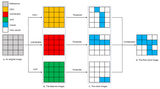
Figure 1.
The cloud detection method based on hybrid multispectral features. (a) An original image. (b) The features images. (c) The cloud images. (d) The final cloud image.
We assume there is an original image with 4 × 4 pixels. The first step is to calculate the three features values respectively and get the three features images. The second step is to detect which pixels are clouds and which are not. The last step is to combine these three cloud images to get the final cloud image, the combined principle is if a pixel has been detected as a cloud pixel in any cloud images, we think it is a cloud pixel in the final cloud image. However, the HOT formula (4) is variant because of the two coefficients ( and ), so how to stabilize these two coefficients is an essential point in the method, which we will introduce in the next section.
2.2. Seasonal HOT Formula
2.2.1. Seasonal Datasets
The first step of the HOT feature algorithm is to select the clear sky area in the image and calculate the clear sky line. However, due to the influence of external factors such as solar irradiation intensity and aerosol concentration, the clear sky area and the clear sky line will be different in each image, so the conventional method needs to select the clear sky area manually. In this section, the method of establishing a clear sky background field is used to determine the clear sky line and HOT feature parameter of each image, which avoids manual selection of clear sky area and improves efficiency. A large number of clear and cloudless multispectral images of the satellite are selected as the data source to establish the seasonal clear sky background field, as Figure 2 shows. After pre-processing and geometric registration, the coordinates of different images have been unified. Then, the blue and red band data sets of all images are averaged separately, and the mean images of the two data sets (clear sky background field) are obtained by C# (a kind of programming language).
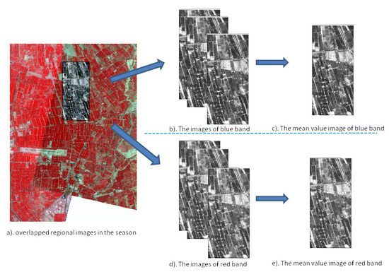
Figure 2.
Seasonal clear sky background field method. (a) overlapped regional images in the season. (b) The images of blue band. (c) The mean value image of the blue band. (d) The images of the red band. (e) The mean value image of the red band.
2.2.2. Linear Regression
The next step is to calculate the clear sky line for every season. Firstly, the red and blue band scatter diagram of all the pixels in the seasonal background field is constructed using the least square method. The result is shown in Figure 3.
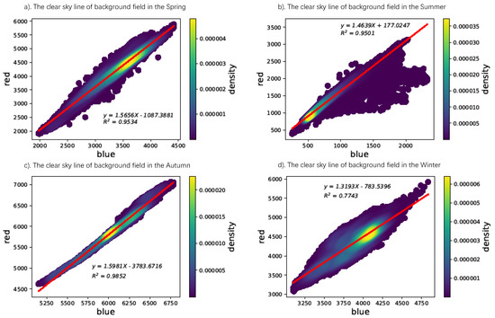
Figure 3.
Clear sky lines for seasonal backgrounds. (a) The clear sky line of background field in the Spring. (b) The clear sky line of background field in the Summer. (c) The clear sky line of background field in the Autumn. (d) The clear sky line of the background field in the Winter.
In Figure 3, the horizontal axis represents the blue band and the vertical axis represents the red band. The red and blue band pixel values of the clear sky background field in each season are linearly correlated. The regression coefficients b and a of the clear sky line equation in each season are shown in Table 4.
Table 4.
The coefficients of clear sky line.
It can be seen from Table 4 that the determinant coefficient R of the clear sky line equation in each season is high, which indicates that the background field can be used as the reference data for calculating the feature value, HOT. From the regression equation of the clear sky lines and Equation (4), the Equations (5) and (6) can be derived. Therefore, the and in Equation (4) can be derived, as Table 5 shows.
Table 5.
The parameters of HOT.
2.3. Dynamic Thresholds
Variability in surface characteristics over the vast territory of China makes using a fixed threshold for cloud detection unreasonable. In theory, there is no fixed threshold for nationwide cloud detection of multispectral features. Therefore, a dynamic threshold calculation method combined with solar elevation angle is adopted.
2.3.1. Coefficients of Formula
Koichi Kawano [22] believes that for visible and near infrared bands, the relationship between local solar elevation angle and image reflectance can be defined by Equation (7).
In the equation, is the reflectance of the pixel, and is the solar elevation angle. The values of and are obtained by linear regression analysis of a series of point pairs composed of and . In this section, 10 high-resolution multispectral images of Heilongjiang in 2015 are selected for band linear fitting, and the coefficients in the equations between solar elevation angle and reflectance in blue, red, green and near infrared bands of GF-1 images are obtained separately, as Table 6 shows.
Table 6.
The coefficient table of sun elevation and reflectance.
2.3.2. Algorithm
The flow chart of cloud detection with dynamic threshold is shown as Figure 4.
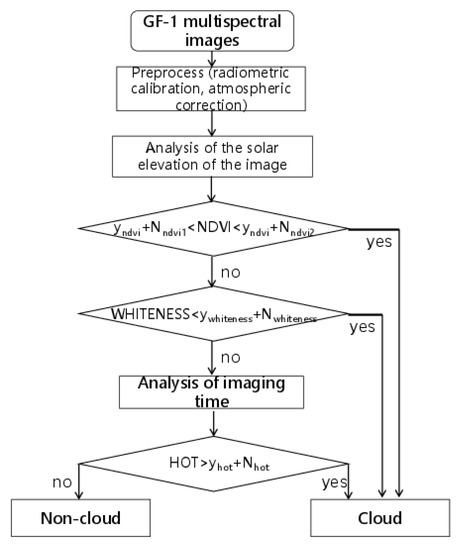
Figure 4.
The flow chart of cloud detection with dynamic threshold.
The algorithm flow of calculating dynamic threshold and the parameters in the Figure 4 are as follows:
- (1)
- suppose that the reference image’s central point is x and solar elevation angle is . After radiation correction and atmospheric calibration, three cloud detection feature parameters are calculated respectively. Then we continually adjust thresholds (t, t, t and t) until the accuracy of cloud detection of the reference image is more than 90% with these thresholds.
- (2)
- (3)
- (4)
- calculate the difference (N) between features of the reference image and the thresholds, as shown in Equation (10).
- (5)
- suppose that the center point of the image (the clouds that need to be detected) is y and the solar elevation angle is . After radiation correction and atmospheric calibration, the pixel values of the ith band of the image’s central point y(y) can be obtained through the Equation (7) and coefficients in Table 6, as shown in Equation (11).
- (6)
- (7)
- calculate the threshold (T) of NDVI, WHITENESS and HOT of the image which is needed to detect clouds, as shown in Equation (13).
When we use this method to detect clouds of GF-1 imageries, we only need to find out the thresholds of the reference image, then we save the thresholds as fixed parameters, there is no need to tune the thresholds every time. After that, we can use this method to automatically calculate the features’ thresholds of each image from the reference image, which make it possible to detect clouds in different images (large-scale area).
3. Results
3.1. Experiment Design
The paper designed three experiments to demonstrate the proposed method has a high accuracy and efficiency. The first experiment is a comparison between the HMF and single features mentioned in Section 2, which can interpret why we chose the HMF rather than a single feature. The second experiment is making a comparison between the proposed method and a random forest method in accuracy and efficiency. The experimental environment is a personal computer with the Ubuntu 14.06 operation system, an 8 GB RAM, an Intel(R) Core(TM) i7-7700HQ CPU and Python 3.6. The third experiment uses the proposed method in parallel to detect clouds in the whole of China, which illustrates that our method can be applied over a large-scale area.
3.2. The Comparative Accuracy and Efficiency
3.2.1. Comparison between the HMF and Single Features
In this section, the experiment data is a GF-1 multi-spectral image with 8 m spatial resolution of TIFF format, randomly selected from Heilongjiang province. The image is shown in Figure 5a. In the image, the underlying surface is vegetation with some scattered thick clouds and a small amount of thin clouds. The image is classified into five types of objects: thick cloud, thin cloud, vegetation, water body and bare land by supervised classification. Then the NDVI, WHITENESS and HOT parameters of the image are calculated. Finally, the best threshold values of the three parameters of the image for cloud recognition are obtained by bisection and visual interpretation respectively: −0.1 < NDVI < 0.21, WHITENESS < 0.1, HOT > 1050, cloud detection results with different feature combinations are shown in Figure 5.
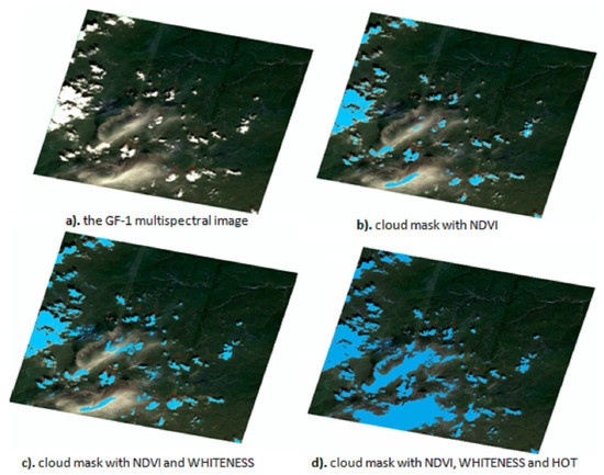
Figure 5.
The cloud detection effect with different feature combinations (The pixel depth of the image in part a is 16 bit unsigned integer, the whole volume of image is about 0.15 GB, the rows and columns of the image are about 4500 × 4500).
In order to quantitatively evaluate the accuracy of cloud detection with combination of different features, ArcGIS random selection and classification evaluation function is used to gather statistics for the accuracy of the cloud detection results of images. In this section, 100 corresponding points were randomly selected from the two images for each type of object and were compared. The results are shown in Table 7, Table 8 and Table 9.
Table 7.
Accuracy assessment of the cloud detection result with NDVI.
Table 8.
Accuracy assessment of the cloud detection result with NDVI and WHITENESS.
Table 9.
Accuracy assessment of the cloud detection result with three feature parameters.
Figure 5b and Table 7 demonstrate that the cloud detection with NDVI can detect thick clouds and non-cloud objects well. The accuracy of thick clouds detection is 84%, but it does not work well on thin clouds detection, with an accuracy of only 35%.
After comparing Figure 5b,c, Table 7 and Table 8, it can be seen that a combination of NDVI and WHITENESS improves cloud detection compared with just using NDVI. However, the detection of thin clouds is unsatisfactory with an accuracy of only 59%.
Through visual interpretation of cloud detection results (Figure 5d), it can be clearly seen that thick clouds or thin clouds in the image are effectively detected and the results of the clouds’ edge detection mask are highly consistent with the shape of clouds’ edge. From Table 9, it can be seen that the detection accuracy of clouds or non-cloud objects is more than 90% by using three multispectral features. Compared with thick clouds, some thin clouds are still misjudged, but the overall accuracy of clouds detection is more than 90%, which can meet the requirements of subsequent agricultural applications.
3.2.2. The Comparison to the Random Forest Method
We also conducted an experiment to compare the proposed method with the accuracy and efficiency of the random forest approach. We adopted the same programming language, Python 3.6, to achieve the two methods. The random forest approach is described in the reference [31], then four randomly selected GF-1 16-m images were used as the experimental data. One of the four images was used to collect the training samples, and other images were used to test the accuracy and the efficiency of cloud detection. The accuracy is shown in Table 10. It can be found that the two methods have no apparent difference when it comes to detecting clouds, but random forest is more likely to categorize crops into clouds by mistake. Furthermore, the average time consumption with random forest to detect clouds for a GF-1 image is 12 h 21 min, but the proposed method only needs 2 h 4 min. Therefore, the proposed method has the advantage of efficient calculation compared to the random forest approach.
Table 10.
A comparison of the proposed method and random forest method
3.3. Large-Scale Cloud Detection
In order to evaluate the cloud detection capability in a large-scale area, some randomly selected GF-1 multispectral remote sensing images in China are used to detect clouds. The results are shown in the Figure 6 and the accuracy assessment is shown in Table 11.
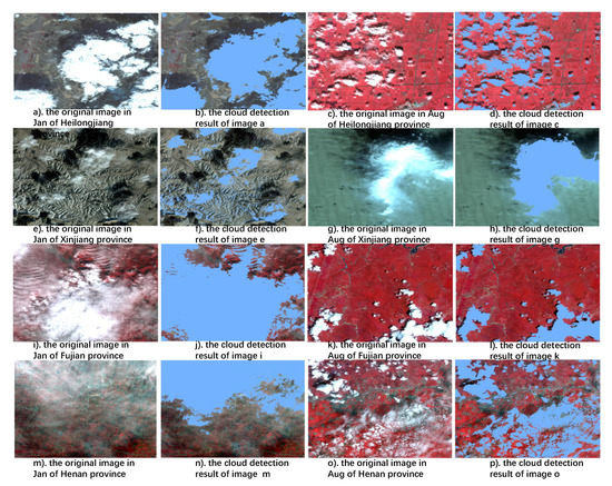
Figure 6.
The contrast of original images and cloud detection results (the columns of the 1st and 3rd are original images, the other columns are corresponding cloud detection results).
Table 11.
Accuracy assessment of the cloud detection result with the hybrid multispectral features with dynamic thresholds.
Through visual interpretation of cloud detection results (Figure 6) and analyzing Table 11, it can be seen that thick cloud detection accuracy can reach 93.8% and thin cloud detection accuracy can reach 87.9%. Although the detection accuracy of thin clouds is slightly lower than that of thick clouds, the overall detection accuracy of cloud pixels is 90.8%, and that of non-cloud pixels is 94.6%, so it can be shown that thick clouds or thin clouds in the nationwide image are effectively detected. At the same time, this section presents statistics on the cloud detection speed of a 8-m multispectral image and a 16-m multispectral image with the number of 1, 20, 50, 100 and 200. The statistical results are shown in the following Figure 7. It can be seen that the computing speed of the cloud detection system can reach the second level in processing GF-1 8-m multispectral images and the minute level for 16-m multispectral images, and the computing efficiency has reached the current application requirements.
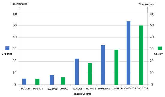
Figure 7.
The cloud detection efficiency for 16-m images/8-m images.
4. Discussion
The fixed thresholds of each feature parameter found in Section 3.2 are partially inconsistent with the range of each parameter corresponding to the cloud in Section 2.1. This is mainly because the data which were used are not the same data, so it shows that although the threshold method can distinguish cloud and non-cloud objects to a certain extent, the thresholds of different regions or different seasons are variable, which implies that there is no fixed threshold for nationwide cloud detection of multispectral features. Thus, the method of cloud detection with a dynamic threshold proposed in this paper is essential, and can calculate the corresponding threshold for each GF-1 remote sensing image.
However, due to the overlap of cloud and snow in spectral characteristics and the lack of the Short Wave Infrared (SWIR) band in the GF-1 images which is needed when calculating the Normalized Difference Snow Index (NDSI), it is easy to make a misjudgement when using this method to detect cloud and snow. The main attempt in this work is to acquire the real reflectance of crops for subsequent agricultural application. If crops are covered by snow, the reflectance of a remote sensing image cannot reflect the real information of a crop, so these pixels cannot be utilized either. Therefore, this kind of misjudgement has a positive impact, which can be ignored in this study. However, for other applications, clouds and snow might need to be distinguished effectively. In this case, interested researchers can consider using texture features to distinguish clouds and snow. Furthermore, cloud shadow is also a challenge in cloud detection. In this paper, the method cannot address this problem. In future work, some feature parameters which can detect cloud shadow will be considered.
In evaluating the accuracy of the cloud detection results, this work and most researchers still choose the corresponding points randomly from an original image and detected image, then evaluate the accuracy by visual interpretation and judge the effect of cloud detection based on the results. Therefore, how to evaluate cloud detection accuracy more objectively is the difficulty of the current research stage, and is also the next research work of this study. This paper establishes a set of parameters from images in Heilongjiang province, even though the nationwide application has demonstrated that this method works. In the future, we would also focus on exploring and researching the differences of these parameters in different regions.
5. Conclusions
Based on the features of the GF-1 satellite sensor and the requirement of cloud detection in agriculture, this paper proposes a cloud detection method based on hybrid multispectral features with a dynamic threshold for GF-1 remote sensing images to achieve the high precision and highly efficient distinction between clouds and crops. Through experiments and analysis of various multispectral features, this work preliminarily shows that NDVI, WHITENESS and HOT provide a certain degree of discrimination between cloud and other ground objects in GF-1 satellite data. Combining this with experimental analysis, this work finds out that the accuracy of cloud detection is the highest when the three features are used in combination, which is more than 90%. In this paper, through the establishment of clear sky background field and linear fitting in four seasons, the corresponding HOT parameter calculation equations in different seasons are obtained. The R of fitting results in spring, summer and autumn all reach above 0.95, the fitting effect is excellent, and the influence of different imaging times on the calculation of HOT parameters is reduced as far as possible. At the same time, this paper adopts an effective method to dynamically acquire the thresholds of NDVI, WHITENESS and HOT according to the change of solar elevation angle, which minimizes the influence of different imaging positions on the three feature parameters’ thresholds. In addition, experiments show that the proposed method can process 8-m and 16-m GF-1 images efficiently, the speed can reach second and minute levels respectively. In terms of accuracy, cloud detections are carried out for random images in China, and the overall cloud detection accuracy is 90.8%. The main contributions of this work as follows: 1. we explored an effective strategy based on previous researchers’ works without any other auxiliary data to detect clouds of the GF-1 images which are not suitable for some popular algorithms. 2. the proposed method has been applied into scientific production and supports other researches in the preprocessing of remote sensing images [33] and crop mapping [38,39].
Author Contributions
Conceptualization, Q.X. and Y.W.; Methodology, Q.X. and Y.W.; Software, D.L., Z.D. and W.L.; Validation, S.Y., Q.X. and Y.W.; Formal Analysis, S.Y.; Investigation, Y.W.; Resources, W.S. and X.Z.; Data Curation, J.H.; Writing–original Draft Preparation, Q.X.; Writing–review and Editing, Q.X., X.Y.; Visualization, Y.W.; Supervision, D.Z.; Project Administration, D.Z.; Funding Acquisition, X.Z. All authors have read and agreed to the published version of the manuscript.
Funding
This research was funded by [National Natural Science Foundation of China] grant number [41771104].
Conflicts of Interest
The authors declare no conflict of interest.
Abbreviations
The following abbreviations are used in this manuscript:
| GF-1 | GaoFen No.1 |
| NDVI | Normalized Difference Vegetation Index |
| HOT | Haze-Optimized Transformation |
| AVHRR | Advanced Very High Resolution Radar |
| NOAA | National Oceanic and Atmospheric Administration |
| MODIS | Moderate Resolution Imaging Spectroradiometer |
| TM | The Thematic Mapper |
| HMF | Hybrid Multispectral Features |
References
- Ye, S.; Zhao, C.; Wang, Y.; Liu, D.; Du, Z.; Zhu, D. Design and implementation of automatic orthorectification system based on GF-1 big data. Trans. Chin. Soc. Agric. Eng. 2017, 33. [Google Scholar] [CrossRef]
- Zeng, C. The Quality Assessment and Feature Analysis of Domestic High Resolution Satellite Images. Master’s Thesis, Chengdu University of Technology, Chengdu, China, 2017. [Google Scholar]
- Bai, Z. Technical characteristics of GF-1 remote sensing satellite. Aerosp. China 2013, 5–9. [Google Scholar]
- Dong, Q.; Yue, C. Image Fusion and Quality Assessment of GF-1. For. Inventory Plan. 2016, 41, 1–5, 10. [Google Scholar] [CrossRef]
- Jia, K.; Liang, S.; Gu, X.; Baret, F.; Wei, X.; Wang, X.; Yao, Y.; Yang, L.; Li, Y. Fractional vegetation cover estimation algorithm for Chinese GF-1 wide field view data. Remote Sens. Environ. 2016, 177, 184–191. [Google Scholar] [CrossRef]
- Li, J.; Chen, X.; Tian, L.; Huang, J.; Feng, L. Improved capabilities of the Chinese high-resolution remote sensing satellite GF-1 for monitoring suspended particulate matter (SPM) in inland waters: Radiometric and spatial considerations. ISPRS J. Photogramm. Remote Sens. 2015, 106, 145–156. [Google Scholar] [CrossRef]
- Chen, N.; Li, J.; Zhang, X. Quantitative evaluation of observation capability of GF-1 wide field of view sensors for soil moisture inversion. J. Appl. Remote Sens. 2015, 9, 097097. [Google Scholar] [CrossRef]
- Wang, M. Study on the Distributions and Physical Properties of Cirrus clouds. Master’s Thesis, Nanjing University of Information Science & Technology, Nanjing, China, 2013. [Google Scholar]
- Chen, X. Research on Recognition Technology of Typtical Ground-based Cloud. Ph.D. Thesis, Southeast University, Nanjing, China, 2015. [Google Scholar]
- Cai, W.; Liu, Y.; Li, M.; Cheng, L.; Zhang, C. A self-adaptive homomorphic filter method for removing thin cloud. In Proceedings of the 2011 19th International Conference on Geoinformatics, Shanghai, China, 24–26 June 2011; pp. 1–4. [Google Scholar] [CrossRef]
- Wang, X.; Li, M.; Tang, H. A modified homomorphism filtering algorithm for cloud removal. In Proceedings of the 2010 International Conference on Computational Intelligence and Software Engineering, Wuhan, China, 10–12 December 2010; pp. 1–4. [Google Scholar] [CrossRef]
- Zhu, Z.; Woodcock, C.E. Object-based cloud and cloud shadow detection in Landsat imagery. Remote Sens. Environ. 2012, 118, 83–94. [Google Scholar] [CrossRef]
- Wang, B.; Ono, A.; Muramatsu, K.; Fujiwara, N. Automated detection and removal of clouds and their shadows from Landsat TM images. IEICE Trans. Inf. Syst. 1999, 82, 453–460. [Google Scholar]
- Zhu, Z.; Woodcock, C.E. Automated cloud, cloud shadow, and snow detection in multitemporal Landsat data: An algorithm designed specifically for monitoring land cover change. Remote Sens. Environ. 2014, 152, 217–234. [Google Scholar] [CrossRef]
- Saunders, R.W.; Kriebel, K.T. An improved method for detecting clear sky and cloudy radiances from AVHRR data. Int. J. Remote Sens. 1988, 9, 123–150. [Google Scholar] [CrossRef]
- Ackerman, S.A.; Strabala, K.I.; Menzel, W.P.; Frey, R.A.; Moeller, C.C.; Gumley, L.E. Discriminating clear sky from clouds with MODIS. J. Geophys. Res. Atmos. 1998, 103, 32141–32157. [Google Scholar] [CrossRef]
- Li, W.; Fang, S.; Dian, Y.; Guo, J. Cloud Detection in MODIS Data Based on Spectrum Analysis. Geomat. Inf. Sci. Wuhan Univ. 2005, 30, 435–438. [Google Scholar] [CrossRef]
- Liu, X.; Wang, Y.; Shi, H.; Long, Z.; Jiang, Z. Cloud Detection over the Southest China Basing on Statistical Analysis. J. Image Graph. 2005, 15, 1783–1789. [Google Scholar]
- Li, C.; Liu, L.; Wang, J.; Song, X.; Wang, R. Automatic detection and removal of thin haze based on own features of Landsat image. J. Zhejiang Univ. Sci. 2006, 40, 10–13. [Google Scholar]
- Yun, Y.; Xia, Y.; Zhang, J.; Pan, Y. Cloud and Cloud Shadow Detection in GF-1 Imagery Using Single-date Method. Remote Sens. Inf. 2017, 32, 35–40. [Google Scholar] [CrossRef]
- Automatic Cloud Detection from MODIS Images; 2004; Volume 5235. [CrossRef]
- Kawano, K.; Kudoh, J.I. Cloud detection method for NOAA AVHRR images by using local area parameters. In Proceedings of the IEEE 2001 International Geoscience and Remote Sensing Symposium (Cat. No. 01CH37217), Sydney, NSW, Australia, 9–13 July 2001; Volume 5, pp. 2155–2157. [Google Scholar] [CrossRef]
- Dybbroe, A.; Karlsson, K.G.; Thoss, A. NWCSAF AVHRR cloud detection and analysis using dynamic thresholds and radiative transfer modeling. Part I: Algorithm description. J. Appl. Meteorol. 2005, 44, 39–54. [Google Scholar] [CrossRef]
- Liu, Z.; Li, Y.; Huang, F. Cloud Detection of MODIS Satellite Images Based on Dynamical Cluster. Remote. Sens. Inf. 2007, 4, 33–35. [Google Scholar]
- Sun, S. A multi-spectral remote sensing imagery cloud detection algorithm based on spectral angle principle. Microcomput. Its Appl. 2017, 36, 16–18. [Google Scholar] [CrossRef]
- Liu, Z.; Han, L.; Zhou, P.; Wang, X.; Wu, T. A Method for Cloud Interpretation in ZY-3 Satellite Imagery and Its Application. Remote Sens. Inf. 2017, 32, 41–46. [Google Scholar] [CrossRef]
- Wu, J. Cloud Detection Algorithm for Domestic High-Resolution Multispectral Image Data. Comput. Netw. 2015, 41, 45–47. [Google Scholar]
- Jin, Z.; Zhang, L.; Liu, S.; Yi, F. Cloud Detection and Cloud Phase Retrieval Based on BP Neural Network. Opt. Optoelectron. Technol. 2016, 14, 74–77. [Google Scholar]
- Yu, W.; Cao, X.; Xu, L.; Bencherkei, M. Automatic cloud detection for remote sensing image. Chin. J. Sci. Instrum. 2006, 27, 2184–2186. [Google Scholar] [CrossRef]
- Wang, W.; Song, W.; Liu, S.; Zhang, Y.; Zheng, H.; Tian, W. A Cloud Detection Algorithm for MODIS Images Combining Kmeans Clustering and Multi-Spectral Thershold Method. Spectrosc. Spectr. Anal. 2010, 31, 1061–1064. [Google Scholar] [CrossRef]
- Fu, H.; Shen, Y.; Liu, J.; He, G.; Chen, J.; Liu, P.; Qian, J.; Li, J. Cloud detection for FY meteorology satellite based on ensemble thresholds and random forests approach. Remote Sens. 2019, 11, 44. [Google Scholar] [CrossRef]
- Ye, S. Research on Application of Remote Sensing Tupu—Take Monitoring of Meteorological Disaster for Example. Ph.D. Thesis, China Agricultural University, Beijing, China, 2016. [Google Scholar]
- Ye, S.; Liu, D.; Yao, X.; Tang, H.; Xiong, Q.; Zhuo, W.; Du, Z.; Huang, J.; Su, W.; Shen, S.; et al. RDCRMG: A Raster Dataset Clean & Reconstitution Multi-Grid Architecture for Remote Sensing Monitoring of Vegetation Dryness. Remote Sens. 2018, 10, 1376. [Google Scholar] [CrossRef]
- Jiang, D.; Wang, N.; Yang, X.; Liu, H. Principles of the Interaction Between NDVI Profile and the Growing Situation of Crops. Acta Ecol. Sin. 2002, 22, 247–252. [Google Scholar]
- Yang, Y.; Zhan, Y.; Tian, Q.; Gu, X.; Yu, T.; Wang, L. Crop classification based on GF-1/WFV NDVI time series. Trans. Chin. Soc. Agric. Eng. 2015, 31, 155–161. [Google Scholar] [CrossRef]
- Gómez-Chova, L.; Camps-Valls, G.; Calpe-Maravilla, J.; Guanter, L.; Moreno, J. Cloud-screening algorithm for ENVISAT/MERIS multispectral images. IEEE Trans. Geosci. Remote Sens. 2007, 45, 4105–4118. [Google Scholar] [CrossRef]
- Zhang, Y.; Guindon, B.; Cihlar, J. An image transform to characterize and compensate for spatial variations in thin cloud contamination of Landsat images. Remote Sens. Environ. 2002, 82, 173–187. [Google Scholar] [CrossRef]
- Yang, N.; Liu, D.; Feng, Q.; Xiong, Q.; Zhang, L.; Ren, T.; Zhao, Y.; Zhu, D.; Huang, J. Large-Scale Crop Mapping Based on Machine Learning and Parallel Computation with Grids. Remote Sens. 2019, 11, 1500. [Google Scholar] [CrossRef]
- Zhang, L.; Liu, Z.; Liu, D.; Xiong, Q.; Yang, N.; Ren, T.; Zhang, C.; Zhang, X.; Li, S. Crop Mapping Based on Historical Samples and New Training Samples Generation in Heilongjiang Province, China. Sustainability 2019, 11, 5052. [Google Scholar] [CrossRef]


© 2020 by the authors. Licensee MDPI, Basel, Switzerland. This article is an open access article distributed under the terms and conditions of the Creative Commons Attribution (CC BY) license (http://creativecommons.org/licenses/by/4.0/).