Analysis of Grassland Degradation in Zona da Mata, MG, Brazil, Based on NDVI Time Series Data with the Integration of Phenological Metrics

 ,
,
Abstract
1. Introduction
2. Materials and Methods
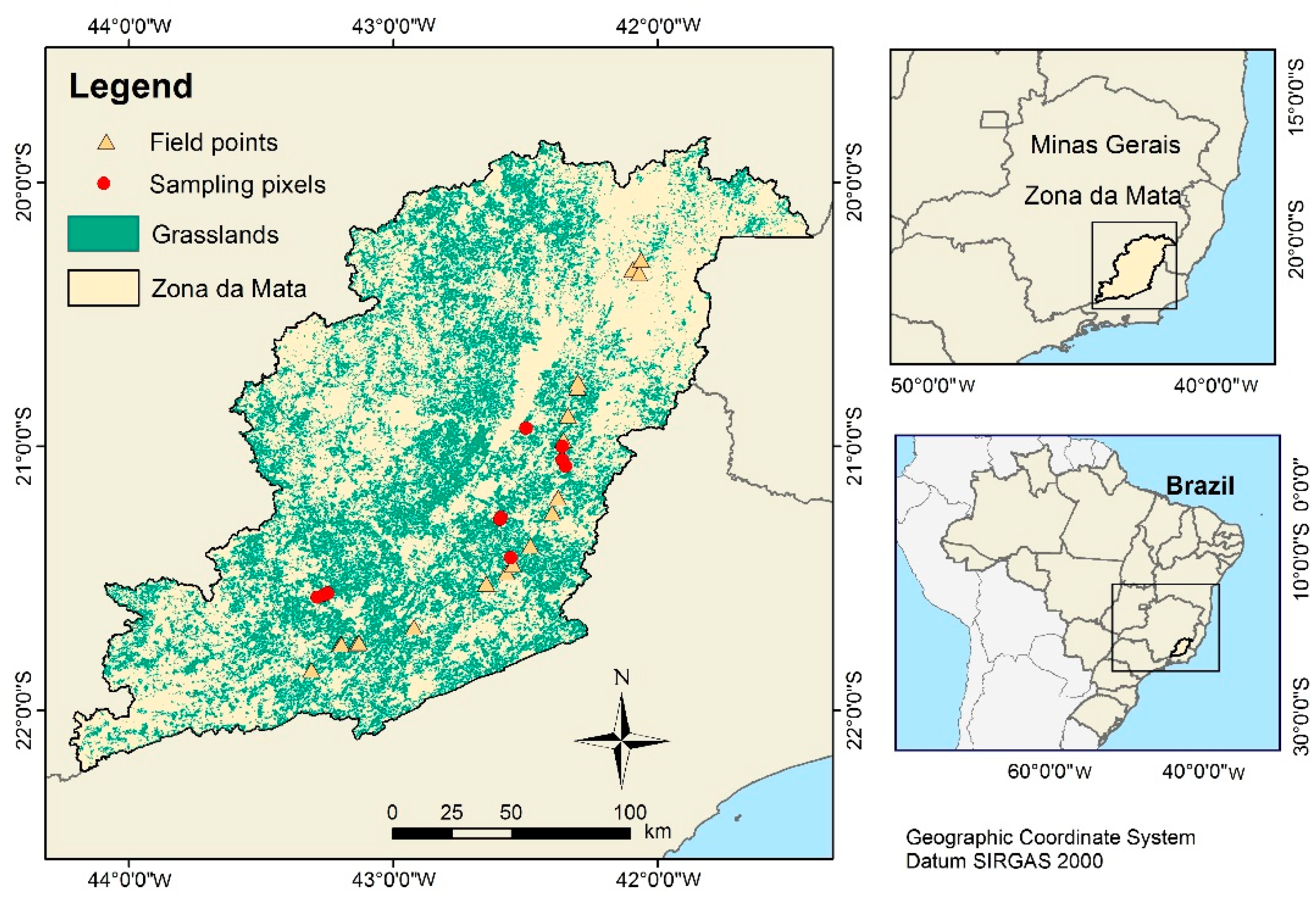
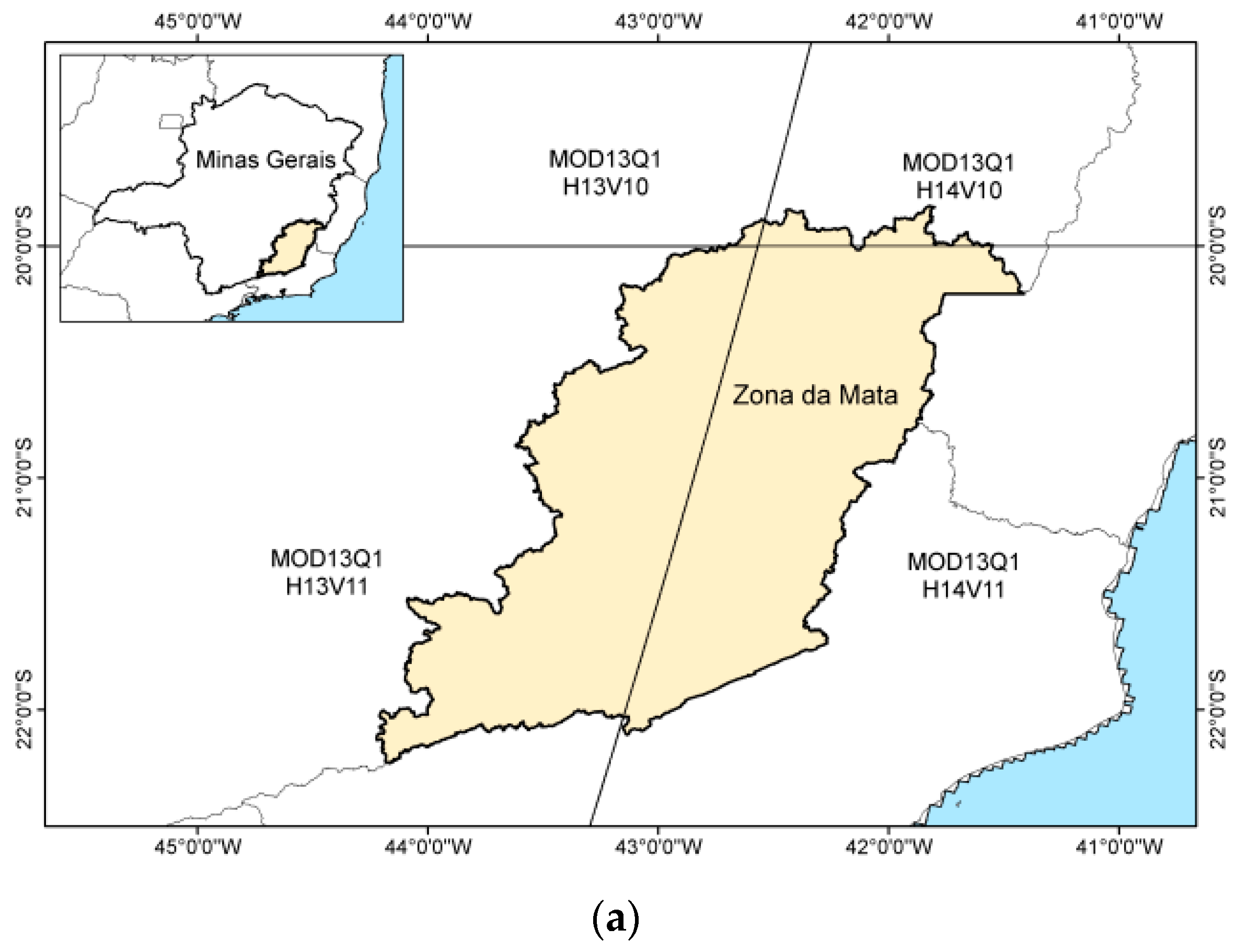
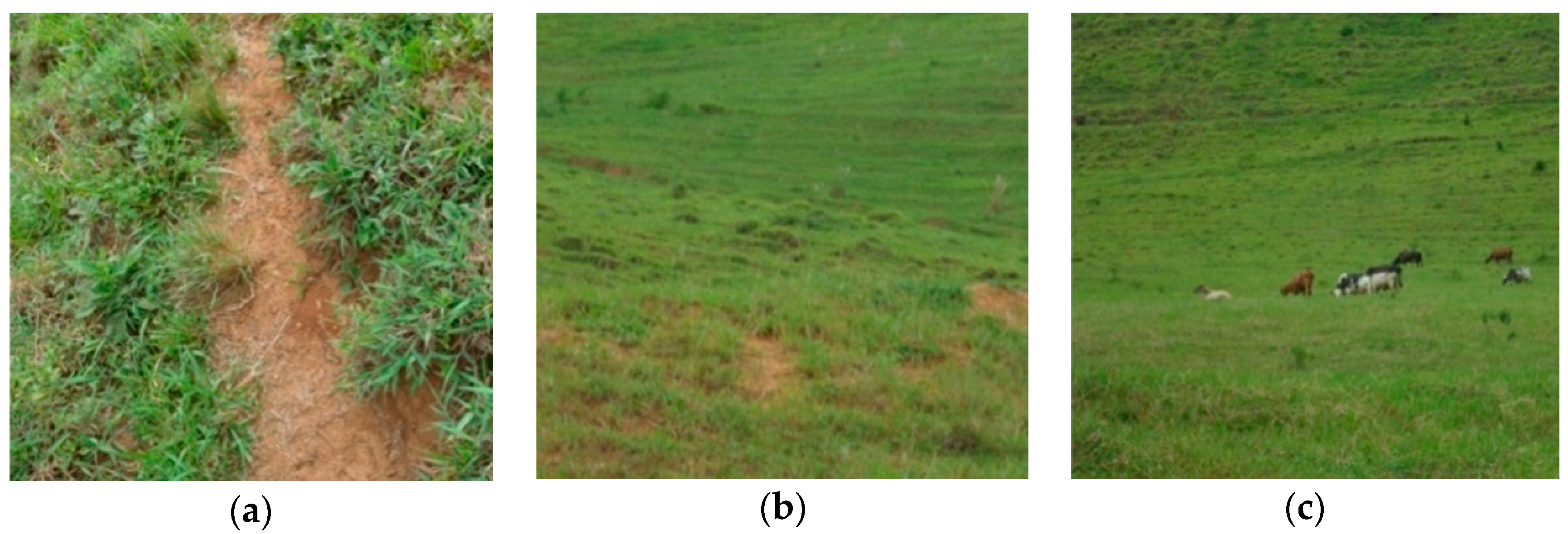
2.1. Study Area
2.2. Materials
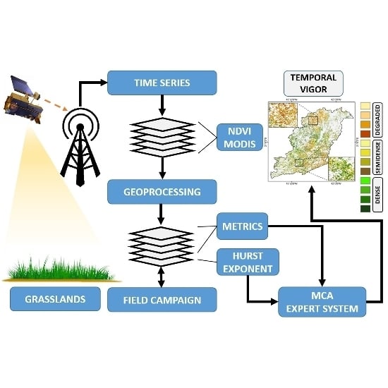
2.3. Methods
2.3.1. Growth Index
2.3.2. Linear Trend: Slope
2.3.3. Exploratory Metrics: Maximum, Minimum, and Mean
2.3.4. Hurst Exponent
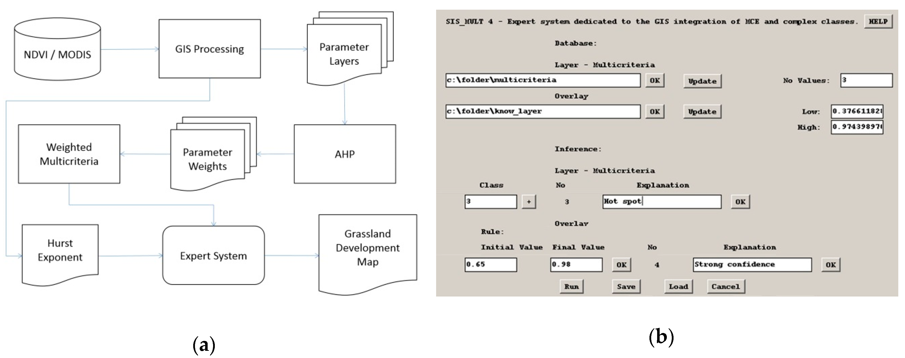
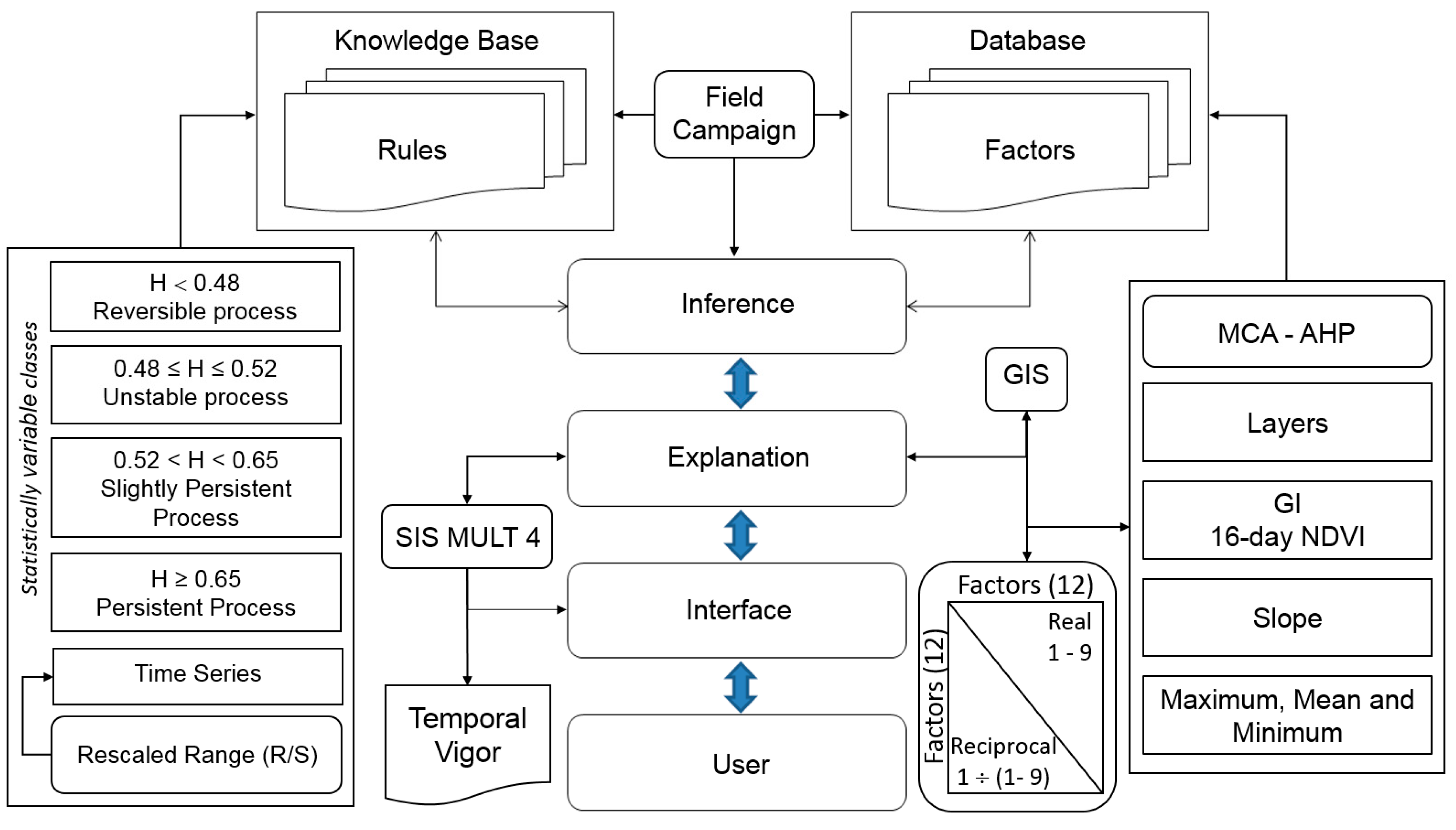
2.3.5. Multicriteria Analysis and Expert System
- Degraded and reversible: The vegetation index decreases over time, with low plant cover; the future trend is an increase in plant cover.
- Degraded and unstable: A decreasing vegetation index with low plant cover and a small or unobservable trend.
- Degraded and slightly persistent: The decreasing vegetation index indicates low plant cover, a moderate trend for maintenance of the degradation process, sparse grasslands, compacted soils, and overgrazing.
- Degraded and persistent: The decrease in the vegetation index shows low plant cover and a strong trend for maintenance of the grassland degradation.
- Semidense and reversible: This class has a moderate to high vegetation index and sparse to semidense plant cover, and it shows a trend toward plant density instability from fallow, burnings, or crop rotation.
- Semidense and unstable: This class is characterized by moderate plant cover and a low or no temporal trend due to complex farming practices such as variations in the cattle stocking rate.
- Semidense and slightly persistent: Areas in this class have moderate plant cover and show a reasonable trend for sustained grassland vigor.
- Semidense and persistent: This class has reasonable plant cover and exhibits a strong trend for sustaining this vegetation condition.
- Dense and reversible: There is a high level of plant cover, but with a trend toward reversal of the plant density over time, from the adjacent management or degradation.
- Dense and unstable: There is a high level of plant cover and a low or no temporal trend.
- Dense and slightly persistent: There is a high level of plant cover and a moderate trend for sustained grassland vigor.
- Dense and persistent: This class has a high level of plant cover and a strong indication for sustained density or a high vegetation index.
3. Results
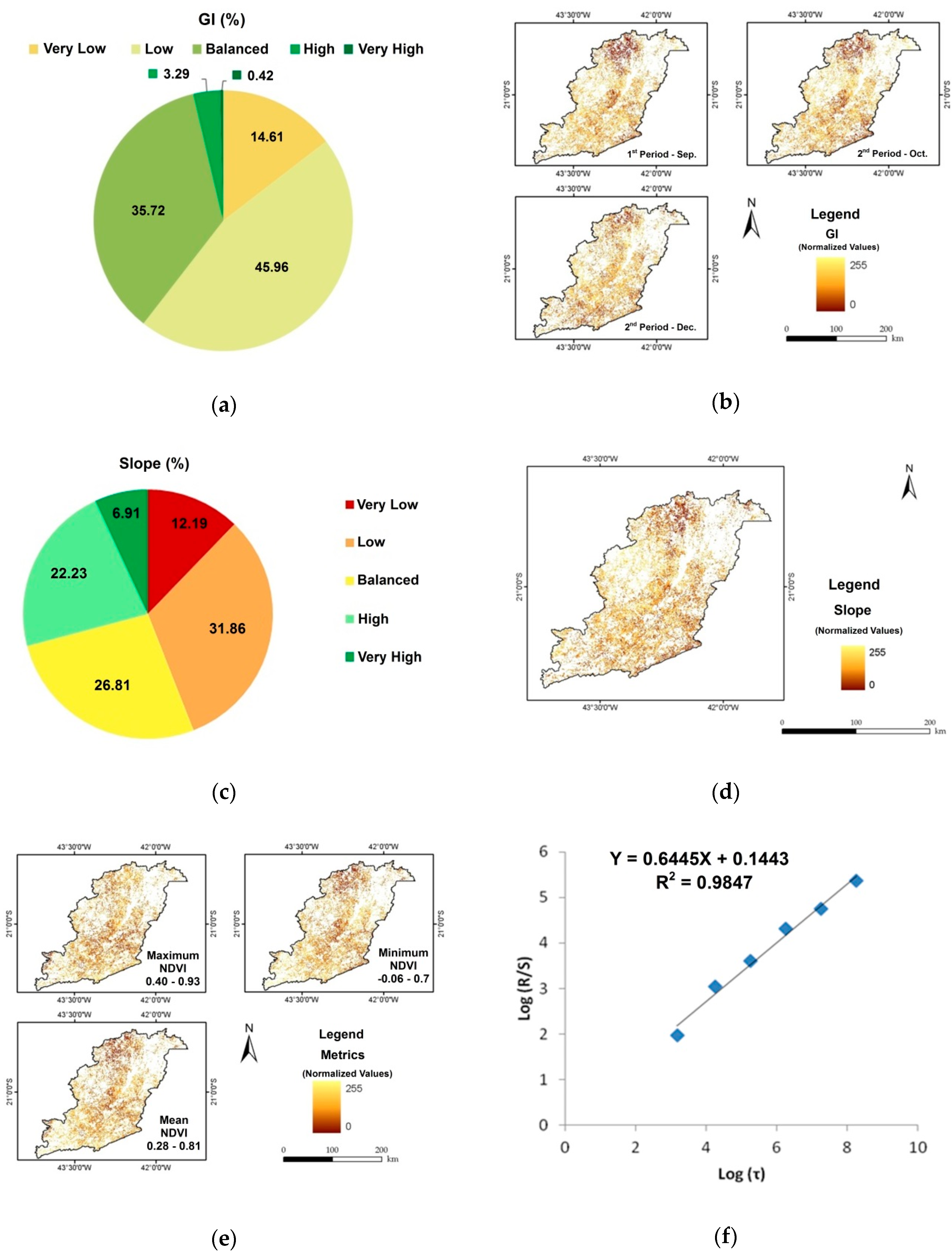
3.1. GI for Spring
3.2. Slope Metrics
3.3. Maximum, Minimum, and Mean NDVI
3.4. Temporal Statistic (H)
3.5. Multicriteria and Expert Systems
3.5.1. MCA
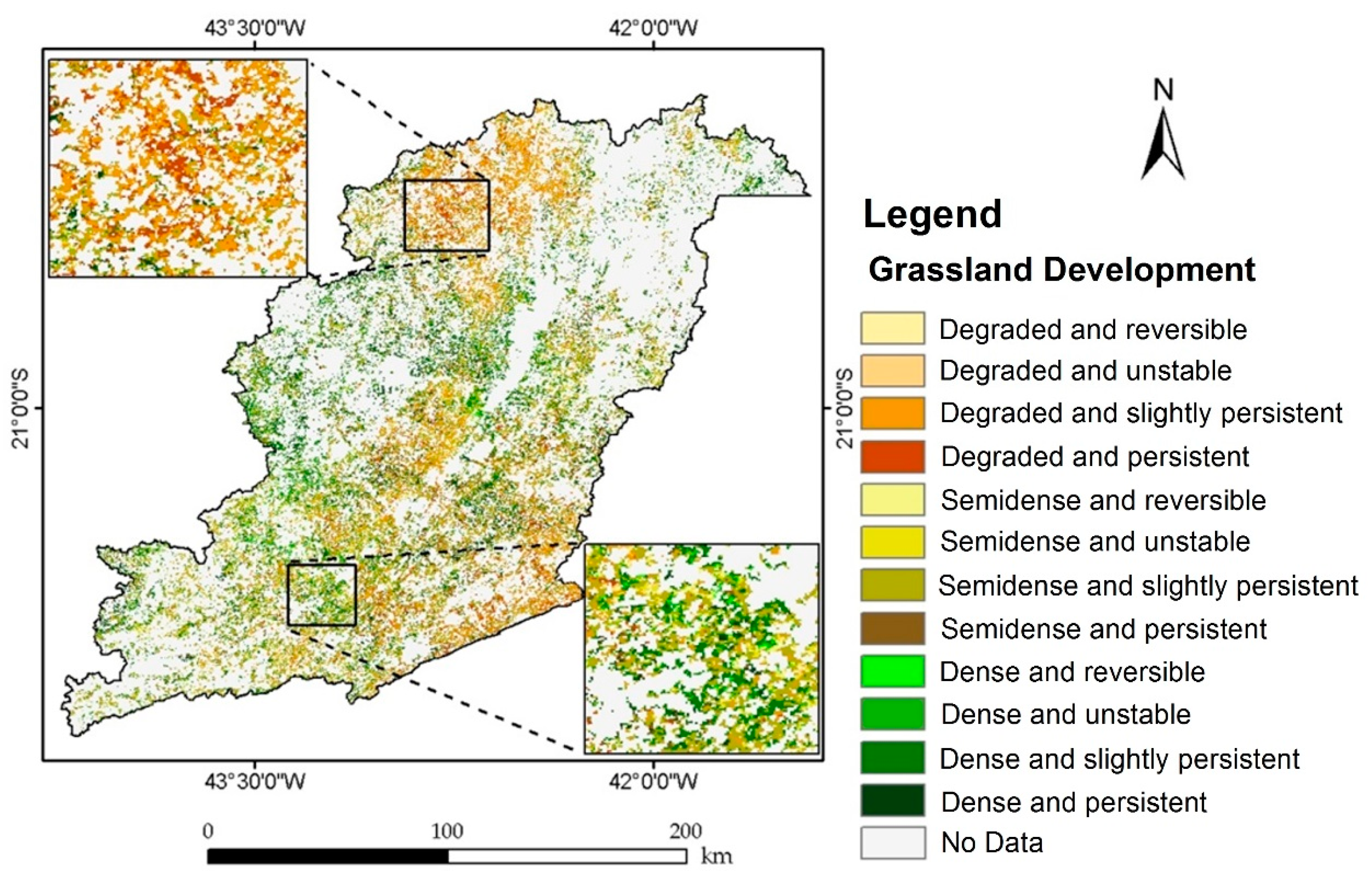
3.5.2. ESS
4. Discussion
5. Conclusions
- Most grasslands in Zona da Mata (approximately 61.5%) are degraded or are undergoing degradation with long-term persistence;
- Approximately 27% of the grasslands presented adequately sustainable density conditions, according to the temporal analysis methods; and
- The phenological metrics based on remote sensing and temporal statistics were used effectively to build a management legend to provide guidelines for decision-making in relation to grassland development derived from NDVI/MODIS data and field evaluations.
Author Contributions
Acknowledgments
Conflicts of Interest
References
- IBGE. Instituto Brasileiro de Geografia e Estatística. Censo Agropecuário. Available online: http://www.ibge.gov.br (accessed on 24 October 2017).
- Li, Z.; Huffman, T.; McConkey, B.; Townley-Smith, L. Monitoring and modeling spatial and temporal patterns of grassland dynamics using time-series MODIS NDVI with climate and stocking data. Remote Sens. Environ. 2013, 138, 232–244. [Google Scholar] [CrossRef]
- Rigge, M.; Smart, A.; Wylie, B.; Gilmanov, T.; Johnson, P. Linking Phenology and Biomass Productivity in South Dakota Mixed-Grass Prairie. Rangel. Ecol. Manag. 2013, 66, 579–587. [Google Scholar] [CrossRef]
- Sellers, P.J. Canopy reflectance, photosynthesis and transpiration. Int. J. Remote Sens. 1985, 6, 1335–1372. [Google Scholar] [CrossRef]
- Sellers, P.J. Canopy reflectance, photosynthesis and transpiration, II The role of biophysics in the linearity of their interdependence. Remote Sens. Environ. 1987, 21, 143–183. [Google Scholar] [CrossRef]
- Sellers, P.J.; Berry, J.A.; Collatz, G.J.; Field, C.B.; Hall, F.G. Canopy reflectance, photosynthesis and transpiration. III. A reanalysis using improved leaf models and a new canopy integration scheme. Remote Sens. Environ. 1992, 42, 187–216. [Google Scholar] [CrossRef]
- Reeves, M.C.; Zhao, M.S.; Running, S.W. Applying improved estimates of MODIS productivity to characterize grassland vegetation dynamics. Rangel. Ecol. Manag. 2006, 59, 1–10. [Google Scholar] [CrossRef]
- Brito, J.L.S.; Sano, E.E.; Arantes, A.E.; Ferreira, L.G. MODIS estimates of pasture productivity in the Cerrado based on ground and Landsat-8 data extrapolations. J. Appl. Remote Sens. 2018, 12. [Google Scholar] [CrossRef]
- Gichenje, H.; Godinho, S. Establishing a land degradation neutrality national baseline through trend analysis of GIMMS NDVI Time-series. Land Degrad. Develop. 2018, 29, 2985–2997. [Google Scholar] [CrossRef]
- Chen, J.; GU, S.; Shen, M.; Tang, Y.; Matsuchita, B. Estimating aboveground biomass of grassland having a high canopy cover. An exploratory analysis of in situ hyperspectral data. Int. J. Remote Sens. 2009, 30, 6497–6517. [Google Scholar] [CrossRef]
- Huang, C.; Geiger, E.L.; Van Leeuwen, W.J.D.; March, S.E. Discrimination of invaded and native species sites in a semi-desert grassland using MODIS multi-temporal data. Int. J. Remote Sens. 2009, 30, 897–917. [Google Scholar] [CrossRef]
- Holm, A.M.; Cridland, S.W.; Roderick, M.L. The use of time-integrated NOAA NDVI data and rainfall to assess landscape degradation in the arid shrubland of Western Australia. Remote Sens. Environ. 2003, 85, 145–158. [Google Scholar] [CrossRef]
- Ratana, P.; Huete, A.R.; Ferreira, L. Analysis of Cerrado physiognomies and conversion in the MODIS seasonal-temporal domain. Earth Interact. 2005, 9, 1–22. [Google Scholar] [CrossRef]
- Clerici, N.; Weissteiner, C.J.; Gerard, F. Exploring the use of MODIS NDVI-based phenology indicators for classifying forest general habitat categories. Remote Sens. 2012, 4, 1781–1803. [Google Scholar] [CrossRef]
- You, X.Z.; Meng, J.H.; Zhang, M.; Dong, T. Remote sensing based detection of crop phenology for agricultural zones in China using a new threshold method. Remote Sens. 2013, 5, 3190–3211. [Google Scholar] [CrossRef]
- Gong, Z.; Kawamura, K.; Ishikawa, N.; Goto, M.; Wulan, T.; Alateng, D.; Yin, T.; Ito, Y. MODIS normalized difference vegetation index (NDVI) and vegetation phenology dynamics in the Inner Mongolia grassland. Solid Earth 2015, 6, 1185–1194. [Google Scholar] [CrossRef]
- USGS. United States Geological Survey. Remote Sensing Phenology. Available online: http://phenology.cr.usgs.gov/methods_metrics.php (accessed on 20 February 2016).
- XU, B.; Yang, X.C.; Tao, W.G.; Miao, J.M.; Yang, Z.; Liu, H.Q.; Jin, Y.X.; Zhu, X.H.; Qin, Z.H.; Lv, H.Y.; et al. MODIS-based remote-sensing monitoring of the spatiotemporal patterns of China’s grassland vegetation growth. Int. J. Remote Sens. 2013, 34, 3867–3878. [Google Scholar] [CrossRef]
- Stow, D.; Daeschner, S.; Hope, A.; Douglas, D.; Petersen, A.; Myneni, R.; Zhou, L.; Oechel, W. Variability of the seasonally integrated normalized difference vegetation index across the north slope of Alaska in the 1990s. Int. J. Remote Sens. 2003, 24, 1111–1117. [Google Scholar] [CrossRef]
- Liu, S.; Wang, T.; Guo, J.; Qu, J.; An, P. Vegetation change based on SPOT-VGT data from 1998–2007, northern China. Environ. Earth Sci. 2010, 60, 1459–1466. [Google Scholar] [CrossRef]
- Zhang, Y.C.; Zhao, Z.Q.; Li, S.C.; Meng, X.F. Indicating variation of surface vegetation cover using SPOT NDVI in the northern part of North China. Geogr. Res. 2008, 27, 745–754. [Google Scholar] [CrossRef]
- Hurst, H.E. The long-term storage capacity of reservoirs. Trans. Am. Soc. Civ. Eng. 1951, 116, 770–799. [Google Scholar]
- Mandelbrot, B.; Wallis, J. Robustness of the rescaled range R/S in the measurement of noncyclic long run statistical dependence. Water Resour. Res. 1969, 5, 967–988. [Google Scholar] [CrossRef]
- Hou, X.; Hana, L.; Gao, M.; Bi, X.; Zhu, M. Application of spatiotemporal data mining and knowledge discovery for detection of vegetation degradation. In Proceedings of the Fuzzy Systems and Knowledge Discovery (FSKD), Yantai, China, 10–12 August 2010; pp. 2124–2128. [Google Scholar] [CrossRef]
- Katsev, S.; L’Heureux, I. Are Hurst exponents estimated from short or irregular time series meaningful? Comput. Geosci. 2003, 29, 1085–1089. [Google Scholar] [CrossRef]
- Souza, S.R.S.; Tabak, B.M.; Cajueiro, D.O. Investigação da memória de longo prazo na taxa de cambio no Brasil. Rev. Bras. Econ. 2006, 60, 193–209. [Google Scholar] [CrossRef]
- Ashutosh, C.; Abhey, R.B.; Dimri, V.P. Wavelet and rescaled range approach for the Hurst coefficient for short and long time series. Comput. Geosci. 2007, 33, 83–93. [Google Scholar] [CrossRef]
- Kale, M.; Butar, F. Fractal Analysis of Time Series and Distribution Properties of Hurst Exponent. Math. Sci. Math. Educ. 2011, 6, 8–19. Available online: http://msme.us/2011-1-2.pdf (accessed on 5 May 2015).
- Flynn, M.N.; Pereira, W.R.L.S. Ecological diagnosis from biotic data by Hurst exponent and the R/S analysis adaptation to short time series. Biomatemática 2013, 23, 1–14. Available online: http://www.ime.unicamp.br/~biomat/bio23_art1.pdf (accessed on 11 June 2015).
- Peng, J.; Liu, Z.; Liu, Y.; WU, J.; Han, Y. Trend analysis of vegetation dynamics in Qinghai-Tibet Plateau using Hurst Exponent. Ecol. Indic. 2012, 14, 28–39. [Google Scholar] [CrossRef]
- Huete, A.R.; Huete, A.; Didan, K.; Miura, T.; Rodriguez, E.P.; Gao, X.; Ferreira, L.G. Overview of the radiometric and biophysical performance of the MODIS vegetation indices. Remote Sens. Environ. 2002, 83, 195–213. [Google Scholar] [CrossRef]
- Malczewski, J. GIS-based multicriteria decision analysis: A survey of the literature. Int. J. Geogr. Inf. Sci. 2006, 20, 703–726. [Google Scholar] [CrossRef]
- Estoque, R.C.; Murayama, Y. Suitability analysis for beekeeping sites in La union, Philippines, using GIS & MCE techniques. Res. J. Appl. Sci. 2010, 5, 242–253. [Google Scholar]
- Murayama, Y.; Thapa, R.B. Spatial Analysis and Modeling in Geographical Transformation Process: GIS-Based Applications, 1st ed.; Springer: Dordrecht, The Netherlands, 2011; Volume 100, ISBN 978-94-007-0670-5. [Google Scholar]
- Plant, R.E.; Vayssières, M.P. Combining expert system and GIS technology to implement a state-transition model of oak woodlands. Comput. Electron. Agric. 2000, 27, 71–93. [Google Scholar] [CrossRef]
- Metternicht, G. Assessing temporal and spatial changes of salinity using fuzzy logic, remote sensing and GIS. Foundations of an expert system. Ecol. Model. 2001, 144, 163–179. [Google Scholar] [CrossRef]
- Yang, X.; Skidmore, A.K.; Melick, D.R.; Zhou, Z.; Xu, J. Mapping non-wood forest product (matsutake mushrooms) using logistic regression and a GIS expert system. Ecol. Model. 2006, 198, 208–218. [Google Scholar] [CrossRef]
- Ahmadia, F.F.; Ebadi, H. Using cognitive information in the expert interface system for intelligent structuring and quality control of spatial data measured from photogrammetric or remotely sensed images. Measurement 2014, 48, 167–172. [Google Scholar] [CrossRef]
- Carvalho, L.M.T.; Fonseca, L.M.G.; Murtagh, F.; Clevers, J.G.P.W. Digital change detection with the aid of multiresolution wavelet analysis. Int. J. Remote Sens. 2001, 22, 3871–3876. [Google Scholar] [CrossRef]
- Gitelson, A.A.; Peng, Y.; Huemmrich, K.F. Relationship between fraction of radiation absorbed by photosynthesizing maize and soybean canopies and NDVI from remotely sensed data taken at close range and from MODIS 250 m resolution data. Remote Sens. Environ. 2014, 147, 108–120. [Google Scholar] [CrossRef]
- Oliveira, J.C.; Epiphanio, J.C.N.; Rennó, C.D. Window Regression: A Spatial-Temporal Analysis to Estimate Pixels Classified as Low-Quality in MODIS NDVI Time Series. Remote Sens. 2014, 6, 3123–3142. [Google Scholar] [CrossRef]
- IBGE. Instituto Brasileiro de Geografia e Estatística. Censo Agropecu. 2015. [Google Scholar]
- Saaty, T.L. The Analytic Hierarchy Process; McGraw-Hill: New York, NY, USA, 1980; p. 176. [Google Scholar]
- Lo, W. Long-term memory in stock market prices. Econometrica 1991, 59, 1279–1313. [Google Scholar] [CrossRef]
- Peters, E.E. Fractal Market Analysis: Applying Chaos Theory to Investment and Economics; Wiley: New York, NY, USA, 1994. [Google Scholar]
- Sánchez, Z.; Trinidad, J.E.; García, P.J. Some comments on Hurst exponent and the long memory processes on capital markets. Phys. A Stat. Mech. Appl. 2008, 387, 5543–5551. [Google Scholar] [CrossRef]
- Liu, S.; Cheng, F.; Dong, S.; Zhao, H.; Hou, X.; Wu, X. Spatiotemporal dynamics of grassland aboveground biomass on the Qinghai-Tibet Plateau based on validated MODIS NDVI. Sci. Rep. 2017, 7, 4182. [Google Scholar] [CrossRef] [PubMed]
- Xin, X.P.; Gao, Q.; Li, Y.Y.; Yang, Z.Y. Fractal analysis of grass patches under grazing and flood disturbance in an alkaline grassland. Acta Bot. Sin. 1999, 41, 307–313. [Google Scholar]
- Soterroni, A.C.; Domingues, M.O.; Ramos, F.M. Estimativa do expoente de Hurst de séries temporais caóticas por meio da transformada wavelet discreta. In Proceedings of the Congresso Temático de Dinâmica, Controle e Aplicações—DINCON, Presidente Prudente, Brazil, 7–9 May 2008; Volume 7, pp. 437–442. [Google Scholar]
- Qi, J.; Yang, H. Hurst exponents for short time series. Phys. Rev. E 2011, 84, 066114. [Google Scholar] [CrossRef] [PubMed]
- Markovic, D.; Koch, M. Sensitivity of Hurst parameter estimation to periodic signals in time series and filtering approaches. Geophys. Res. Lett. 2005, 32, 17401. [Google Scholar] [CrossRef]
- Calijuri, M.L.; Melo, A.L.O.; Lorentz, J.F. Identificação de áreas para implantação de aterros sanitários com uso de análise estratégica de decisão. Inform. Públ. 2002, 4, 231–250. [Google Scholar]
- Moura, A.C.M. Reflexões metodológicas como subsídio para estudos ambientais baseados em Análise de Multicritérios. In Proceedings of the Simpósio Brasileiro de Sensoriamento Remoto, Florianópolis, Brazil, 21–26 April 2007; Volume 13, pp. 2899–2906. [Google Scholar]
- Saaty, T.L. Relative measurement and it’s generalization in decision making why pairwise comparisons are central in mathematics for the measurement of intangible factors—the Analitic Hierarchy/Network Process. Rev. Real Acad. Cienc. Exactas Fis. Y Nat. Ser. A. Mat. 2008, 102, 251–318. [Google Scholar] [CrossRef]
- Sartori, A.A.C.; Silva, R.F.B.; Zimback, C.R.L. Combinação linear ponderada na definição de áreas prioritárias à conectividade entre fragmentos florestais em ambiente SIG. Rev. Árvore 2012, 36, 1079–1090. [Google Scholar] [CrossRef]
- Rabuske, R.A. Inteligência Artificial; UFSC: Florianópolis, Brazil, 2000. [Google Scholar]
- Andrade, G.A.P.; MAPA, S.; Almeida, P.E.M.; Moura, A.C.M. Sistema Especialista para determinação do índice de potencial de expansão urbana para unidade territorial. In Proceedings of the Congresso Brasileiro de Cartografia, Rio de Janeiro, Brazil, 21–24 October 2007; Volume 23. [Google Scholar]
- Andrade, R.G.; Leivas, J.F.; Garçon, E.A.M.; Silva, G.B.S.; Loebmann, D.G.S.W.; Vicente, L.E.; Bolfe, E.L.; Victoria, D.C. Monitoramento de Processos de Degradação de Pastagens a Partir de Dados Spot Vegetation; Boletim de Pesquisa e Desenvolvimento; EMBRAPA—Monitoramento por Satélite: Campinas, Brazil, 2011. [Google Scholar]
- Parente, L.; Ferreira, L. Spatial and Occupation Dynamics of the Brazilian Pasturelands Based on the Automated Classification of MODIS Images from 2000 to 2016. Remote Sens. 2018, 10, 606. [Google Scholar] [CrossRef]
- Pereira, O.J.R.; Ferreira, L.G.; Pinto, F.; Baumgarten, L. Assessing Pasture Degradation in the Brazilian Cerrado Based on the Analysis of MODIS NDVI Time-Series. Remote Sens. 2018, 10, 1761. [Google Scholar] [CrossRef]


| Numerical Scale | Importance Criteria | Process |
|---|---|---|
| 1 | Equal | Both factors contribute equally |
| 3 | Weak | One factor is more important than the other |
| 5 | Strong | One factor is much more important than the other |
| 7 | Very Strong | One factor is significantly more important than the other |
| 9 | Extremely Strong | One factor is much more significant and important than the other |
| 2, 4, 6, 8 | Intermediaries between the criteria | Weighted gradient between factors |
| N | 3 | 4 | ... | 7 | 8 | 9 | 10 | 11 | 12 |
| RI | 0.52 | 0.89 | ... | 1.35 | 1.40 | 1.45 | 1.49 | 1.51 | 1.54 |
| M Classes Temporal Vigor | H < 0.48 Antipersistence | 0.48 ≤ H ≤ 0.52 Random | 0.52 < H < 0.65 Low Persistence | H ≥ 0.65 Persistence |
|---|---|---|---|---|
| Low | Degraded and reversible | Degraded and unstable | Degraded and slightly persistent | Degraded and persistent |
| Medium | Semidense and reversible | Semidense and unstable | Semidense and slightly persistent | Semidense and persistent |
| High | Dense and reversible | Dense and unstable | Dense and slightly persistent | Dense and persistent |
| Hurst Class | Area (ha) | Area (%) |
|---|---|---|
| H < 0.48 | 29,956.25 | 2.47 |
| 0.48 ≤ H ≤ 0.52 | 105,575.00 | 8.70 |
| 0.52 < H < 0.65 | 833,768.75 | 68.71 |
| H ≥ 0.65 | 244,206.25 | 20.12 |
| Total | 1,213,506.25 | 100.00 |
| Factors | Weight | Product | Ratio |
|---|---|---|---|
| 1st Sep. | 0.107 | 1.363 | 12.755 |
| 2nd Sep. | 0.100 | 1.279 | 12.844 |
| 1st Oct. | 0.100 | 1.279 | 12.844 |
| 2nd Oct. | 0.093 | 1.204 | 12.892 |
| 1st Nov. | 0.088 | 1.134 | 12.852 |
| 2nd Nov. | 0.084 | 1.080 | 12.925 |
| 1st Dec. | 0.075 | 0.981 | 13.109 |
| 2nd Dec. | 0.071 | 0.934 | 13.221 |
| Slope | 0.150 | 2.069 | 13.819 |
| Maximum | 0.054 | 0.694 | 12.818 |
| Minimum | 0.040 | 0.519 | 12.400 |
| Mean | 0.038 | 0.461 | 12.241 |
| CI | 0.0812 | CI/RI = 0.05 |
| Temporal Vigor | ||
|---|---|---|
| Class - MCA | Area (ha) | Area (%) |
| Low | 286,031 | 23.57 |
| Mean | 564,025 | 46.48 |
| High | 363,450 | 29.95 |
| Total | 1,213,506 | 100.00 |
| Class | Area (ha) | Area (%) |
|---|---|---|
| Degraded and reversible | 4662.50 | 0.39 |
| Degraded and unstable | 18,256.20 | 1.50 |
| Degraded and slightly persistent | 204,838.00 | 16.88 |
| Degraded and persistent | 58,275.00 | 4.80 |
| Semidense and reversible | 17,893.80 | 1.47 |
| Semidense and unstable | 58,956.20 | 4.86 |
| Semidense and slightly persistent | 404,662.00 | 33.35 |
| Semidense and persistent | 82,512.50 | 6.80 |
| Dense and reversible | 7393.30 | 0.61 |
| Dense and unstable | 28,362.50 | 2.34 |
| Dense and slightly persistent | 224,269.00 | 18.48 |
| Dense and persistent | 103,425.00 | 8.52 |
| Total | 1,213,506.00 | 100.00 |
© 2019 by the authors. Licensee MDPI, Basel, Switzerland. This article is an open access article distributed under the terms and conditions of the Creative Commons Attribution (CC BY) license (http://creativecommons.org/licenses/by/4.0/).
Share and Cite
Hott, M.C.; Carvalho, L.M.T.; Antunes, M.A.H.; Resende, J.C.; Rocha, W.S.D. Analysis of Grassland Degradation in Zona da Mata, MG, Brazil, Based on NDVI Time Series Data with the Integration of Phenological Metrics. Remote Sens. 2019, 11, 2956. https://doi.org/10.3390/rs11242956
Hott MC, Carvalho LMT, Antunes MAH, Resende JC, Rocha WSD. Analysis of Grassland Degradation in Zona da Mata, MG, Brazil, Based on NDVI Time Series Data with the Integration of Phenological Metrics. Remote Sensing. 2019; 11(24):2956. https://doi.org/10.3390/rs11242956
Chicago/Turabian StyleHott, Marcos C., Luis M. T. Carvalho, Mauro A. H. Antunes, João C. Resende, and Wadson S. D. Rocha. 2019. "Analysis of Grassland Degradation in Zona da Mata, MG, Brazil, Based on NDVI Time Series Data with the Integration of Phenological Metrics" Remote Sensing 11, no. 24: 2956. https://doi.org/10.3390/rs11242956
APA StyleHott, M. C., Carvalho, L. M. T., Antunes, M. A. H., Resende, J. C., & Rocha, W. S. D. (2019). Analysis of Grassland Degradation in Zona da Mata, MG, Brazil, Based on NDVI Time Series Data with the Integration of Phenological Metrics. Remote Sensing, 11(24), 2956. https://doi.org/10.3390/rs11242956