Article

Multi-Scale Association between Vegetation Growth and Climate in India: A Wavelet Analysis Approach

1
Department of Civil Engineering, Indian Institute of Technology Bombay, Mumbai, Maharashtra 400076, India
2
NASA Ames Research Center, Moffett Field, CA 94035, USA
3
Bay Area Environmental Research Institute, Moffett Field, CA 94035, USA
4
Centre for Biodiversity and Conservation, Ashoka Trust for Research in Ecology and the Environment (ATREE), Bengaluru, Karnataka 560064, India
5
Department of Civil Engineering, North Eastern University, Boston, MA 02115, USA
6
Interdisciplinary Program in Climate Studies, Indian Institute of Technology Bombay, Mumbai, Maharashtra 400076, India
*
Author to whom correspondence should be addressed.
Remote Sens. 2019, 11(22), 2703; https://doi.org/10.3390/rs11222703
Submission received: 16 September 2019 / Revised: 30 October 2019 / Accepted: 6 November 2019 / Published: 18 November 2019
(This article belongs to the Special Issue Remote Sensing of Tropical Phenology)

Abstract

:
Monsoon climate over India has high degree of spatio-temporal heterogeneity characterized by the existence of multi-climatic zones along with strong intra-seasonal, seasonal, and inter-annual variability. Vegetation growth of Indian forests relates to this climate variability, though the dependence structure over space and time is yet to be explored. Here, we present a comprehensive analysis of this association with quality-controlled satellite-based remote sensing dataset of vegetation greenness and radiation along with station based gridded precipitation datasets. A spatio-temporal time-frequency analysis using wavelets is performed to understand the relative association of vegetation growth with precipitation and radiation at different time scales. The inter-annual variation of forest greenness over the Tropical India are observed to be correlated with the seasonal monsoon precipitation. However, at inter and intra-seasonal scales, vegetation has a strong association with radiation in regions of high precipitation like the Western Ghats, Eastern Himalayas, and Northeast hills. Forests in Western Himalayas were found to be correlated more on the winter precipitation from western disturbances than the south west monsoon precipitation. Our results provide new and useful region-specific information for dynamic vegetation modelling in the Indian monsoon region that may further be used in understanding global vegetation-land-atmosphere interactions.

Graphical Abstract

1. Introduction

A significant fraction of the Indian population depends on forest resources, which according to the India State of Forest Report, 2017 [1] is 21.54% of the total geographical area. These forests are also important biodiversity hotspots [2]. Studies across the globe have shown that the structure and distribution of forests are dependent on the climate patterns; however, any such analysis specific to Indian forest is yet to be performed. The climate in India is characterized by strong seasonality due to the southwest Indian summer monsoon rainfall that occurs during June to September, contributing to 80% of total annual rainfall [3]. The summer monsoon rainfall has variability at both inter-annual and intra-seasonal scales. Inter-annual variability results in surplus and deficit monsoon years in India, whereas the intra-seasonal variability results in active and break periods with high spatial variability [4]. Northeast monsoon resulting from the reversal of wind direction during withdrawal phase of southwest monsoon contributes to the annual rainfall during months of October to December in the Southern parts of India [5,6]. Western disturbances that originate in the Mediterranean Sea cause rainfall in northwestern parts of the country during January and February [7,8]. Hence, Indian climate has a wide spatial heterogeneity and this might affect the dependence of forest growth across the forest regions in the country.
The role of climate variables on the vegetation growth vary significantly across different global climatic zones. In humid temperate biomes, for example, temperature is the primary factor controlling the seasonality of vegetation growth and shifts in the onset of growth cycle have been observed in response to global warming over these regions [9,10]. However, water availability controls the vegetation growth in arid and semiarid ecosystems and seasonally dry tropical climates [11,12,13]. The tropical forests show significant dependence on the precipitation pattern predominantly due to the vegetation structure and species composition [14,15,16]. The species densities were found to increase with increasing precipitation, and the co-existence of the different species is facilitated by a lesser competition for water and low growth rate of understory plants due to less available light [17,18]. Gentry (1988) [16] found a nearly linear relationship of vegetation with precipitation to shift to an asymptotic behavior when the precipitation exceeds 4000 mm/year and concluded that the richness of species in neo-tropical forests is more dependent on precipitation than on soil properties. The regional precipitation gradients can also have indirect effects on leaf functions by controlling the light and nutrient availability. Recent studies in the global tropical forests highlight the role played by radiation on vegetation dynamics, when there is an adequate moisture supply [19,20,21]. It was found that even though the lowest enhanced vegetation index (EVI) in water-limited regions was observed in dry months, the same is not the case when precipitation was observed to be higher than 2000 mm yr-1 [19,21]; the seasonal radiation then act as the climatic control on the forest greening. The same has been confirmed with the help of flux tower observations showing leaf flushing and higher photosynthesis rates in dry seasons [19]. More than 90% of the African tropical evergreen forests, 78% of South East Asian, and 59% of Amazonian forests are below this 2000 mm/year threshold indicating a high water sensitivity of tropical forests in these regions. Nemani et al. (2003) [22] concluded that the water availability is the primary limiting factor for vegetation growth for over 40% of the Earth’s vegetated surface by calculating the relative contributions of different factors using bioclimatic indices. However, they pointed out that the effect of temperature and radiation too cannot be neglected as they have an influence over 33% and 27% of the Earth’s vegetated surface. The findings from the Indian region denoted that the water availability and solar radiation co-limit the vegetation growth and the nearly constant cloud cover limits the incoming solar radiation. Nemani et al. (2003) [22] also analyzed the variation of these factors over the period 1982 to 1999 using analyses data and suggested that wetter rainfall regimes due to changing monsoon dynamics and increase in solar radiation under climate change scenarios for the Indian region can potentially boost the vegetation productivity. However, they did not quantify the relative contributions of the different factors at multiple time scales.
Prasad et al. (2008) [23] concluded that the distribution of forests in the Western Ghats biodiversity hotspot in India is dependent on regional climatic patterns. Regions with an annual rainfall greater than 2000 mm are mostly covered by evergreen forests with a maximum of 10% decline in canopy during dry season. However, in the drier parts of Western Ghats, which are comprised mainly of deciduous forests or savanna woodlands, the greenness is mainly controlled by the precipitation regime. Prasad et al. (2005, 2007) [24,25] conducted studies to understand the relationship between NDVI and climate variables for various forest types in India by regression and correlation analysis. They, however, did not consider the variation of vegetation greenness with climate variables at different temporal scales, which will help us to understand how the diverse forests ecosystems react to shocks from the climate system at different time scales and how fast can they recover, thus understanding the resilience of specific forest ecosystem. We present here the first study to address this multi-scale response of vegetation greenness to precipitation and radiation in India with data acquired from remote sensing platforms.
The conventional approach to understand the multi-scale variability of variables is the use of frequency domain with Fourier transforms. However, the Fourier transform is not capable to specify the temporal location of a particular frequency as it analyzes the signal globally. It is also very sensitive to the changes in function. Fourier transforms are less applicable for non-stationary signals like climate and vegetation variables as it considers the entire series together and makes it more computationally expensive. Hence, wavelet transform, which considers the signal as functions with varying window lengths to transform it into a time-frequency domain, is employed in the current study. Furon et al. (2008) [26] highlighted the use of wavelet analysis in the study of multi-scale and non-stationary processes over various spatial and temporal domain. The significance and validity of wavelet analysis have been discussed over the years [27,28,29]. Wavelet analysis is widely employed in the fields of meteorology [30,31,32,33,34,35,36,37], oceanography [38,39], and geophysics [40,41]. A study conducted by Martínez and Gilabert (2009) [42], analyzed the NDVI time series using the wavelet transform to determine the dynamics of vegetation at different time scales and to identify the phenological cycle. Application of wavelets in understanding the association of vegetation growth with climate at multiple time scales is limited and we present the same for Indian forest regions.

2. Materials and Methods
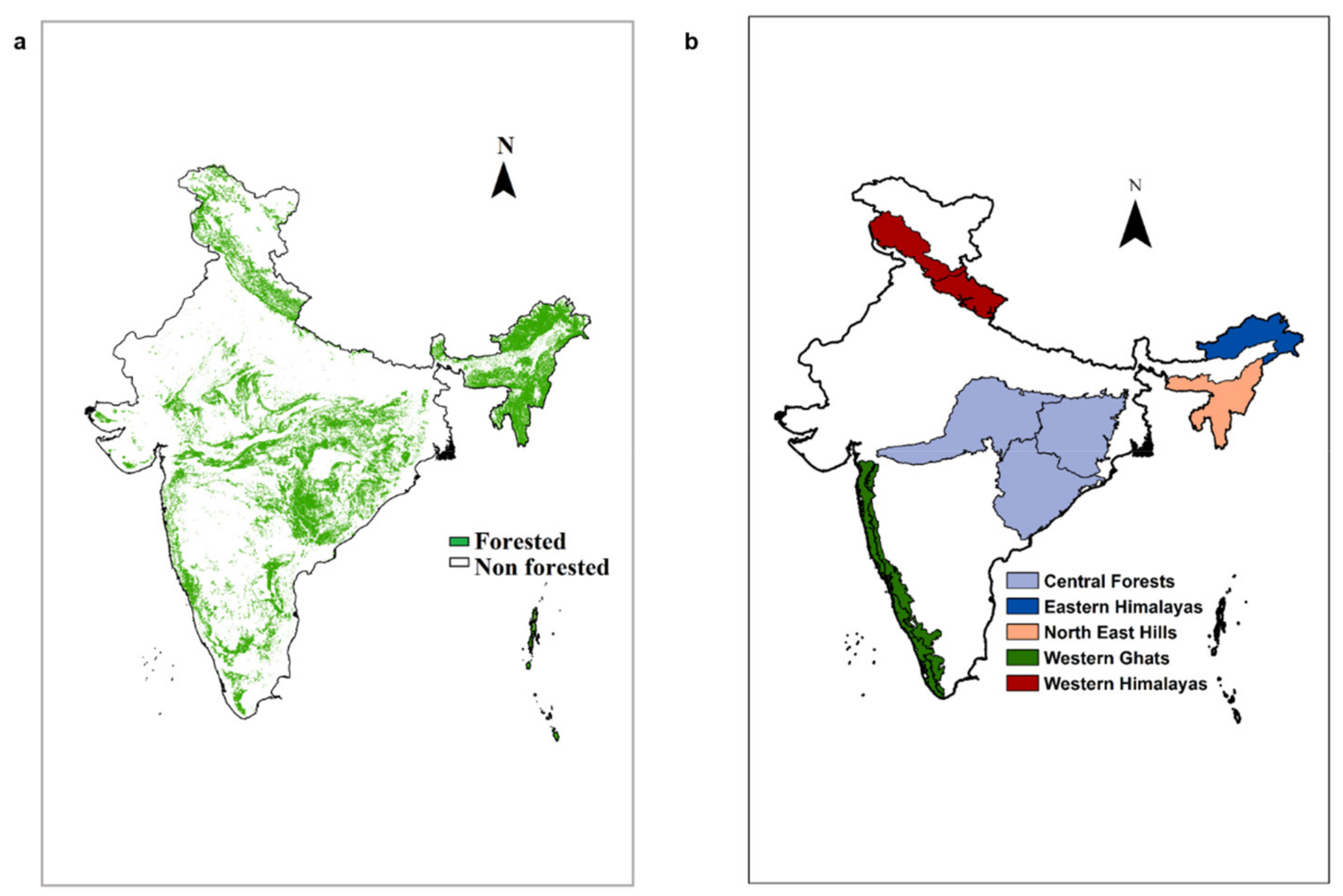
2.1. Study Region

Almost 21.5% of the Indian land mass which spreads over the tropical and sub-tropical zones of the globe is covered by forests. The forest pixels in the country, consisting of deciduous broad and needle-leaved forests, evergreen broad and needle-leaved forests, mixed forests, and mangroves are extracted from a land use land cover (LULC) map provided by Roy et al. (2015) [43] (Figure 1a) and divided into five zones based on the biogeographic classification of Rodgers et al. (2002): Western Ghats forests (WG), central forests (CF), Western Himalayan forests (WH), Eastern Himalayan forests (EH), and forests of Northeast hills (NEH) (Figure 1b).

2.2. Datasets

Daily gridded precipitation at 0.25° resolution, developed from station data is provided by the India Meteorological Department [44]. Daily direct normal irradiance (DNI), which is the amount of solar radiation received per unit area of a surface held perpendicular to radiation, is considered as a proxy for radiation in the current study. It is developed using observations from the Meteosat weather satellite and is provided at 10 km resolution by the National renewable energy laboratory (NREL) National solar radiation database (NSRDB) [45]. Sixteen-day composite enhanced vegetation index (EVI) at 250 m resolution is obtained from MOD13Q1 product [46] of the moderate-resolution imaging spectroradiometer (MODIS) from NASA’s Terra satellite. Considered an indicator of the vegetation greenness, EVI is a measure of the photosynthetically active radiation (PAR) absorbed by chlorophyll. It is defined as:
E V I = G N I R R E D N I R + C 1 R E D C 2 B L U E + L
where G is the gain factor; NIR, RED, and BLUE are the atmospherically corrected reflectance; L is the canopy background adjustment; C1 and C2 are coefficients for atmospheric correction due to aerosol resistance. EVI’s widely used predecessor, NDVI (normalized difference vegetation index), becomes saturated at higher levels of greenness. The inclusion of atmospheric and canopy corrections in the EVI calculation improves sensitivity in high biomass regions. In a comparative study between the two indices, Xiao et al. (2005) [47] concluded that NDVI is unskilled in representing subtle changes in the canopy of wet evergreen forest, which is a major forest type in India. A quality filtering is further employed to remove the effects of clouds, aerosols, and other atmospheric corrections. Based on the availability of both climate and vegetation data, our study is performed over a period of 11 years from 2003 to 2013. The daily precipitation and DNI data are converted to 16-day data by accumulating and averaging over 16 days, respectively, to reach a consensus between the temporal resolutions of the different data.

2.3. Quality Filter

A quality filter provided with the MODIS EVI product specifies the pixel-wise product quality. Applying this filter to forest pixels extracts only high-quality pixels for the study. The bits of the quality assurance (QA) filter correspond to vegetation index (VI) quality, VI usefulness, aerosol quantity, adjacent clouds, mixed clouds, and possible shadow. The minimum quality requirements, as mentioned by Didan et al. (2015) [46], are considered to filter the pixels. Pixels with high VI quality or those which can be accepted by cross-checking with the other quality parameters are only considered. VI usefulness takes into account several conditions including aerosol quantity, atmospheric correction conditions, cloud cover, shadow, and sun-target-viewing geometry. While both low and intermediate aerosol quantity is considered acceptable, the presence of adjacent clouds, mixed clouds, and possible shadow are considered to contaminate the pixel and preclude its use for further analysis.

2.4. Wavelet Analysis

The geophysical processes driving precipitation, radiation, and EVI have variations at multiple time scales and a time-frequency analysis is required to understand this variability. The conventional Fourier transforms consider the entire series as infinite to get time-frequency signals. The spectral composition of the signal is identified without providing the temporal localization of the components in Fourier transforms. On the contrary, variation at different scales can be represented as functions of time corresponding to the periodic components in wavelet analysis [29,31]. Wavelets have varying window lengths in time and frequency domains; thus, a better time localization of different frequencies is possible as compared to Fourier transforms. The window length determines the time and frequency resolution that can be achieved. A narrow window can achieve better time resolution, capable of analyzing high-frequency components, whereas a wider window is capable in low-frequency component identification. In wavelet transform, a signal is decomposed into wavelets φ(t). A wavelet function has zero mean and is localized in both time and frequency. It is a function of translation (τ) and scale (a). Translation parameter is a measure of time and depicts the time shift in the varying window, whereas scale is the inverse of frequency.
φ a , τ t = 1 a φ t τ a
The size of the varying window depends on the frequency to be analyzed. For analyzing high frequencies, narrower windows are employed for better time resolutions. However, at low frequencies, better frequency resolution is given priority and wider windows are selected. For a given mother wavelet, for a time series x(t), the wavelet transform is performed as:
W x a , τ = 1 a + x t φ t τ a d t =   + x t φ a , τ t d t
where the * denotes the complex conjugate form of the function. The mother wavelet considered in the current study is the Morlet wavelet (with frequency as 6), which is ideal for feature extraction and provides a good balance between time and frequency localization. Non-dimensional frequency of 6 satisfies the admissibility condition (zero mean and localized in both time and frequency space) for Morlet wavelet, resulting in a wavelet scale comparable to the Fourier period. The continuous wavelet transform (CWT) normally have edge effects as the beginning and the end of the time series, as it assumes the data to be cyclic. The best way to reduce edge effects is to incorporate longer signals so that it will not affect the part of the signal we are interested in. Another solution is to pad the signals with sufficient zeroes to increase the total length to next higher power of 2 before doing the wavelet transform and then remove them afterward. Padding with zeroes increases discontinuities near the edge points and at larger scales, more zeroes enter the signal, decreasing the amplitude. Cone of influence is the area where the edge effects are important, outside which it can be neglected [29], and is determined as where the wavelet power caused by discontinuities at edges has dropped to e−2 of the value at edge [48]. The statistical significance of a wavelet spectrum is generally determined using the null hypothesis that the signal is stationary and the red noises in the signal can be easily modeled using first order auto regressive functions.
To examine the relationship between the time series of two variables in time–frequency space, cross wavelet transform and wavelet coherence are employed [48], using the Matlab Toolbox provided by Grinsted et al. (2004) [48]. The cross wavelet transform, which identifies the cross-wavelet spectrum, is defined as:
W x , y a , τ = W x a , τ W y a , τ .
Cross wavelet coherency is the correlation between the spectra of two time series [49]. After normalization by individual spectra, cross wavelet coherency takes a value ranging between 0 and 1. Liu (1994) [50] defined cross wavelet coherency as follows:
Γ = W x a , τ W y a , τ W x a , τ W y a , τ .
Since the “wavelet-based quantities” vary in time, they could be used to study the transient association between two signals [50]. To determine the temporal variation of correlation between two non-stationary signals, a smoothing function can be further provided to the wavelet and cross wavelet spectrums. A value of 1 for wavelet coherence indicates a perfect linear correlation between the two signals at the particular time and frequency, while phase difference implies a possible lag between the two signals. Cross wavelet analysis has been employed in applications with non-stationary variables, such as to determine the effect of changing climate on the discharge patterns at continental and regional scales [51,52], understanding rainfall–ground water interactions at different soil depths [53] and the role played by different plant functional types in these interactions [54].

3. Results and Discussions

We apply the wavelet analysis to the natural forested pixels, which are comprised of deciduous broad and needle-leaved vegetation, evergreen broad and needle-leaved vegetation, mixed forests, and mangroves, as shown in Figure 1a, after spatially identifying them as five regions. The radiation received over the Indian landmass is highly affected by the precipitation distribution due to cloud cover. The monsoon precipitation and radiation are found to have a negative correlation of 0.6, indicating the negative impacts of precipitation on radiation. A wavelet analysis of both the variables highlighted the anti-phase nature of both the signals at inter-seasonal and annual timescales represented by the large width of the significant band of higher coherence in Figure S1.

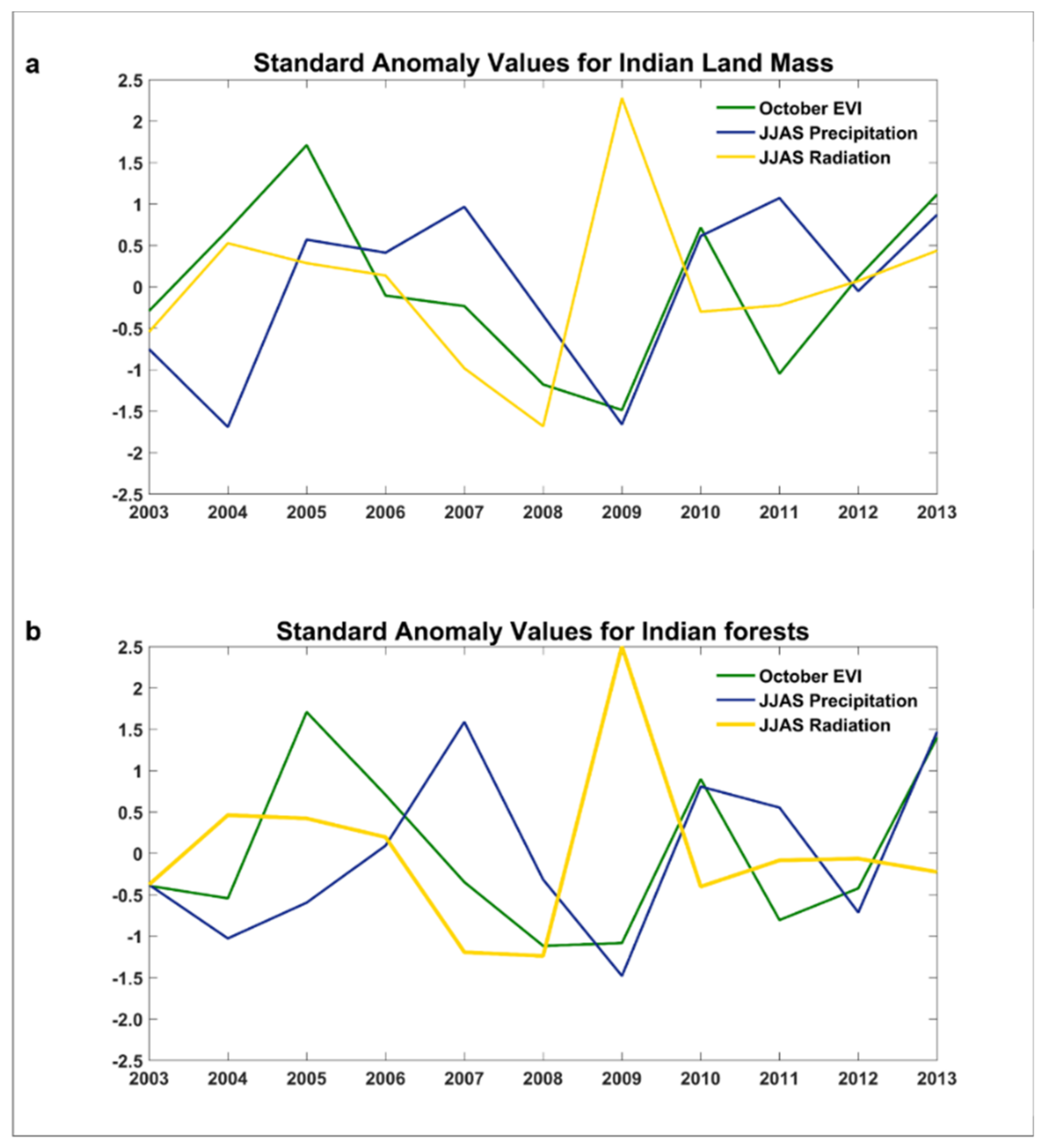
3.1. Multi-Scale Temporal Variation

The vegetation achieves the maximum greenness during the monsoon months (June to September (JJAS)); however, due to the extended cloud cover, its value might be compromised. Hence, the October EVI is considered for understanding the inter-annual variability, taking into account the maximum greenness in vegetation and the quality of EVI data. The inter-annual variability of standard anomalies of October EVI over the entirety of India is compared with the standard anomalies in precipitation and radiation values during monsoon months (June to September, Figure 2a). A clear association of EVI with radiation in addition to precipitation is visible over the years. A deviation from the same is observed in 2009, when a large negative EVI anomaly existed even with a large positive radiation anomaly. This is attributed to the low greenness observed in the previous year (2008) with less precipitation and radiation followed by a very weak monsoon precipitation in 2009, which could not recover the vegetation greenness. This suggests low resilience of vegetation to severe climatic shocks and lingering stresses and how the control on vegetation switches from radiation to precipitation during the periods of low water availability. This dependence on moisture was observed further in 2010, even during a positive precipitation anomaly, suggesting the memory of the land ecosystems with respect to previous cumulative climatic stress and time to recover. To understand the association of vegetation with climate variables in the relatively less human-dominated ecosystems, a similar comparison is done for the forested pixels as shown in Figure 2b. The inter-annual variability of the forest greenness, too, cannot be explained either by precipitation or radiation alone. However, their response is different compared to entire landmass where anthropogenic activities play a major role. The relative role played by precipitation and radiation can be dependent on the regional climate and given the large spatial heterogeneity in monsoon precipitation over India, a region-specific analysis of forests needs to be done.
To analyze the relative influences of precipitation and radiation on vegetation, we conduct a study on the five forest regions in India (Figure 3), considering only the forest pixels shown in Figure 1a. The years are separated based on the anomalies from the multi-year mean monsoon precipitation (or radiation) as positive and negative years. The EVI climatology for years with positive and negative anomalies in precipitation (or radiation) in monsoon months are plotted separately for all the forest regions, with bands representing the variation from the multi-year mean for the various anomaly cases. Different phenology cycles in the four cases (positive and negative anomaly years of precipitation and radiation respectively) indicate that the inter-annual variabilities of precipitation and radiation have impacts on the inter-annual variability of forest greenness; however, it is difficult to get a one-to-one correspondence due to the complex interactions of multiple bio-geophysical processes. It is observed that the composite of EVI in the central forests has higher variability during the greening phase (period before the peak of growing season, where there is an increase in plant greenness) in years with negative anomalies in the monsoon precipitation. Higher variability in the EVI during browning phases is observed for years with negative radiation anomalies. The browning phase (period after the peak of growing season, where there is a decline in plant greenness), also witnesses a higher EVI during the years with positive precipitation anomalies and negative radiation anomalies. The climatology of EVI for all cases are similar in the central forests, which may be attributed to the seasonal nature of the dry deciduous vegetation in the region. However, the variability in EVI values across different years is very high during the growing period, in all cases of precipitation and radiation anomalies. This suggests the influence of other factors like soil moisture availability, local circulation pattern, etc., which have to be addressed while modelling the vegetation in this region. A higher pre-monsoon precipitation, during March through May (MAM), is favorable for the greening of central forests (Figure S2), with an advance in peak during positive MAM precipitation anomaly years compared to negative MAM anomaly years.
A growing season could not be established for the Eastern and Western Himalayas because of the evergreen broad-leaf and needle-leaf trees in the region. A higher band width indicating larger inter-annual variability in Eastern Himalayas (Figure 3c,d), may be attributed to the influence of factors like soil moisture. The relatively less variations in EVI (represented in terms of band width of the climatology plot in Figure 3e,j) in the Western Himalayas proposes that either the EVI has remained stable inter-annually or the variations of EVI are almost fully explained by the variations of precipitation and radiation in this region. Precipitation from the western disturbances during January–February also has an impact on vegetation in the Western Himalayas (Figure S3). Though the climatology is similar in all cases, a positive precipitation and radiation anomaly in January and February (JF) leads to higher EVI values during the two months and a seasonal response similar to those in monsoon months.
Forests in Northeast hills show a fluctuating variability patterns across all the years, with similar EVI climatology for positive precipitation/negative radiation anomalies and negative precipitation/positive radiation anomalies. The co-occurrence of positive precipitation anomalies and negative radiation anomalies in Northeast Hills indicates the possible dimming effect of clouds. The variability bands in this region, however, are narrow, suggesting that the vegetation dynamics are mainly controlled by precipitation and radiation.
The disparity between EVI bands in positive and negative radiation anomaly years in deciduous and evergreen forests of Western Ghats show a high association with the inter-annual variability of radiation in monsoon season. A wider variation band is observed for positive radiation anomaly years than for negative radiation anomaly years, although the climatology in both the cases are similar. The variability hints influence of other factors, such as soil moisture availability during high radiation periods. There is a temporal advancement in the first of the two EVI local maxima in the years with positive monsoon precipitation anomalies, signaling a faster greening with higher precipitation. This pattern is also observed in years with positive pre-monsoon (MAM) precipitation anomalies.
To understand the seasonal association of vegetation with precipitation, the mean change in EVI between monsoon months (JJAS) and pre-monsoon months (MAM), is calculated as:
d e l E V I = E V I J J A S E V I M A M .
Positive values of delEVI indicate the dependence of vegetation on summer monsoon precipitation, whereas negative values of delEVI suggest lack of dependence on summer monsoon and a possible dependence on radiation and non-monsoonal precipitation (Figure 4). Forest pixels are not isolated in understanding the inter-seasonal dependence. The Eastern Himalayas, the Northeast hills, and some parts of Western Ghats region, which receive the majority of annual rainfall in the monsoon months, have a mean decrease in EVI, suggesting radiation dependence of vegetation in high precipitation regions [19]. This is also in agreement with the findings of Xiao et al. (2005) [47] for the moist evergreen forests in Brazil, where they observe a higher photosynthesis rate in the dry season than the wet season. Moreover, most of the over-story species in the region demonstrate dry season leaf flushing [55] and may be another reason for the higher EVI during pre-monsoon months. The southern coasts of Tamil Nadu also have negative mean change values, as these coasts receive the majority of annual precipitation from the Northeast monsoon during October to December and, hence, the delEVI values do not prove dependence of vegetation on radiation.
The spatial mean of multi-year averages of precipitation, radiation, and EVI values of the forest pixels are calculated for the five regions (Figure 5) to understand differences in forest phenology. The mean percentage of high-quality pixels denote the effect of clouds on the EVI satellite product; with the maximum effect visible during monsoon months due to extended cloud cover. The EVI climatology in central Forests (Figure 5a) and Western Ghats (Figure 5d) follow that of precipitation, except at peak values, highlighting that the radiation acts as a limiting factor during periods of high-water availability. The number of high-quality pixels remain significantly high in the central forests, thus suggesting that the observation is not affected by data quality; however, a decline in the high-quality pixels is observed in Western Ghats. The Eastern Himalayas and Northeast hills (Figure 5b,c), receive very high precipitation and demonstrate fluctuating EVI values, which cannot be explained by the climatology of either precipitation or radiation individually, indicating combined effect of both the variables. The local minima of EVI, corresponding to the maximum precipitation and minimum radiation in both the regions, supports the association of EVI with radiation. However, the number of high-quality pixels is found to be reduced during the latter half of monsoon period and such quality issues may also add to the uncertainty in responses of radiation to EVI. The response of forests in Eastern Himalayas, Northeast hills, and Western Ghats imply a weaker influence of precipitation on vegetation above a threshold precipitation value of 2000 mm/year as found by Guan et al. (2015) [19] and is marked by a transition phase with fluctuating EVI in the growing season. Vegetation greenness in the Western Himalayas is mainly associated with rainfall values as seen from the climatology pattern in Figure 5e. This highlights that the vegetation is moisture limited in the regions with low precipitation. We also find a large decrease in the number of high-quality pixels in the Western Himalayas during the period of western disturbances (December to February) possibly due to cloud cover. The region, which has a mountainous terrain, has the lowest number of high-quality pixels compared to other regions, thus revealing the shortcoming of MODIS data in mountainous terrains.

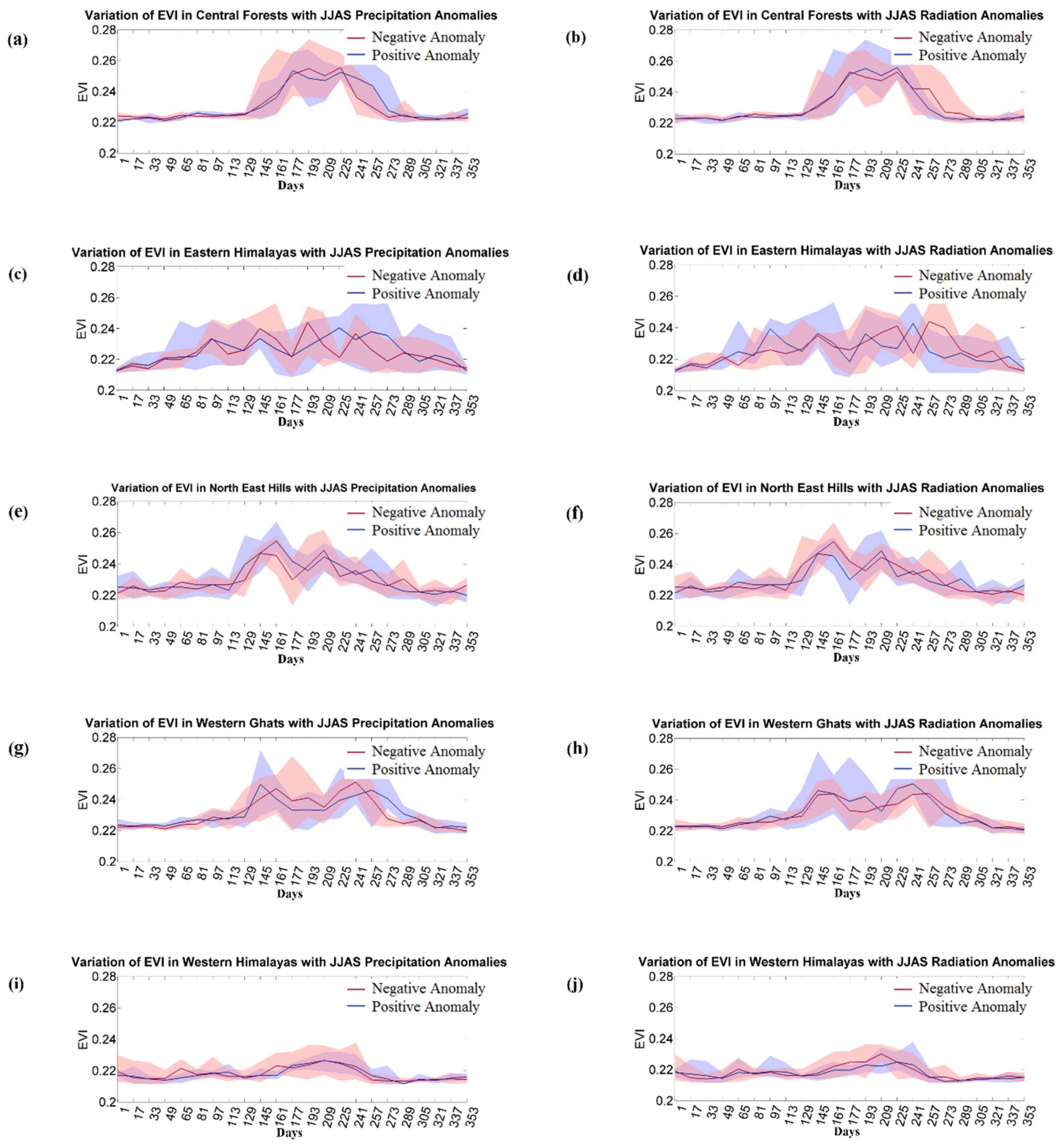
3.2. Wavelet Analysis

Cross wavelet analysis is employed to understand the degree of association of vegetation with precipitation and radiation patterns using 16-day data over a period of 11 years from 2003 to 2013 (253 time steps). Here, continuous wavelet transform (CWT) using Morlet as the mother wavelet is performed on EVI, precipitation, and radiation data. Since the study is based on 16-day EVI data, the period obtained from wavelet analysis needs to be multiplied by 16 to obtain actual periodicity of the events. Since the length of the datasets is very short, the role of edge effects will be significant. Hence the cone of influence is determined to exclude edge effects, depicted with a lighter shade. The significant levels are constant between periods 16–32, for all the study regions and the edge effects might not be affecting the spectrum at large scales where its influence is generally higher. The 5% significance level against red noise is marked with a thick contour. As the CWT power spectrum shown in Figure S4 has a maximum power during a period between 256 to 512 days (period ranging from 16 to 32), it indicates an annual periodicity for the vegetation events throughout the study period, except for the Western Himalayas (affected by westerly disturbances). A few significant periodicities are present at lower time scales in all regions except the Western Himalayas. The wavelet power spectra of Western Himalayas have two major bands, one corresponding to an annual periodicity in some years and the other to a seasonal periodicity of almost 160 days controlled by western disturbances, even though all features are not significant (Figures S5e and S6e). This is suggestive of a seasonality in the EVI pattern in Western Himalayas controlled by the analogous features in the CWTs of precipitation and radiation in these regions.
Interdependencies among two signals can be quantified by the calculation of wavelet transform coherences (WTC). Figure 6 represents the power spectra of WTC between EVI and precipitation for the entire study period and the average coherence values for durations at different periodicities. A larger value of WTC denotes a higher correlation between power spectra of the two variables at the corresponding time and frequency; hence, the relationship at multiple time scales over the study period can be identified. The period at which the maximum coherence is observed can be identified by multiplying the periodicity obtained from WTC analysis with 16 (as the data interval is 16 days). Furthermore, the arrows represent the phase angle between the two signals, with horizontal arrows to the right indicating the signals to be in phase and those to the left as anti-phase in nature. Signals at an angle can either denote a time lag or a lack of association between the two signals. Significant WTCs were observed in the central forests for periodicity ranging from 128 to 512 days (period ranging from 8 to 32 in Figure 6a) for the entire study duration. Larger coherence values having periodicity greater than 256 days depict an annual cycle for vegetation in the central forests. The arrows oriented to the right highlight that the signals are in phase, representing an association of vegetation with the precipitation pattern. However, minor shifts were observed at lower periodicities or seasonal scale (64 to 128 days indicated by a period range of 4 to 8 in Figure 6a). This may be suggestive of the role played by other climatic or environmental factors during periods of high moisture availability. Eastern Himalayas, Northeast hills, and Western Ghats, however, have narrower spectra of high coherency with periodicity greater than 256 days (period greater than 16 in Figure 6c,e,g), which is visible for the entire study duration. The discontinuous multiple patches of high coherency at smaller periodicities propose that the role of seasonal precipitation vary across the years. The EVI and precipitation signals in the Eastern Himalayas and Western Ghats (Figure 6c,g) are in phase at higher periodicities, indicating a close association with precipitation and vegetation at annual scales. However, their behaviors are different when the smaller patches of lower periodicities are considered. This insinuates the influence of other factors such as local circulation and soil moisture on the smaller scale seasonal variations. The EVI and precipitation signals in Northeast hills (Figure 6e) follow a more complex relationship, wherein the signals are in phase during the beginning and end of the study period with a slight deviation in phase angle during the intermediate period. However, the role of edge effects on this pattern is not clear, even though we consider only regions outside the cone of influence. Guan et al. (2015) [19] observed that in regions of high precipitation, the dependency of vegetation on precipitation shifts to radiation dependence. The forests in Northeast hills, being the recipient of very high rainfall, may hence be limited by the available radiation, even at larger periodicities and hence an out-of-phase behavior between EVI and precipitation. The Western Himalayas (Figure 6i), however, has two spectral bands of high coherence spread almost throughout the study duration, suggesting the presence of a seasonal relationship in addition to the annual cycle. Hence, two peaks are visible in the WTC-period curve (Figure 6j), when averaged over the study duration. This can be attributed to the influence of western disturbance on the vegetation pattern of Western Himalayas, though the region is evergreen in nature. EVI and precipitation signals in Western Himalayas are not in phase and whether it be a time lag between the two signals or a lack of any association between them, merits further study. The climatology plots in Figure 5e suggest an association of EVI with precipitation, which supports the existence of a lag between the precipitation and vegetation signals for Western Himalayas.
In most of the regions, wavelet coherence between radiation and EVI signals at periods with high duration are anti-phase, implying that lesser radiation favors vegetation growth at an inter-annual scale (Figure 7). The phase angles for Eastern Himalayas are, however, slightly deviated from anti-phase (Figure 7c) due to a time lag between the two signals or a lack of association between them. The transient phase in the EVI climatology of Eastern Himalayas during monsoon months may be cited as the reason for large variation observed in EVI climatology in Eastern Himalayas. Isolated events of smaller periods, however, have phase angles in the opposite direction, proposing that the role played by radiation shifts at smaller time scales. The Western Himalayas (Figure 7i), like in the case of the EVI‒precipitation relationship, has two bands; however, the smaller band at lower periodicity is not spread across the entire time period as in the case of EVI‒precipitation. The maximum WTC between EVI and radiation in Western Himalayas is higher than that between EVI and precipitation. The seasonal band, however, has a higher WTC between EVI and precipitation suggesting a more limiting role played by precipitation on the Western Himalayan forests during western disturbances than the annual cycle. The transient phases of vegetation greenness, indicated by fluctuating EVI during the monsoon months in Eastern Himalayas and Western Ghats (Figure 5b,d) are visible from the time-averaged WTC values of EVI and precipitation, which show a periodicity at a seasonal scale. The transient phase of vegetation greenness in Northeast hills (Figure 5c) is clearly visible in the time-averaged WTC values of EVI and radiation, thus showing the higher radiation dependence of the region. Significant coherence values and out-of-phase behavior at periods at lower periodicities also point to a complex relationship between EVI and radiation at inter-seasonal scales. The EVI in central forests, however, exhibits no prominent seasonal dynamics, in agreement with the findings in Figure 3 and Figure 5. Hence, a shift in the role played by precipitation and radiation on controlling vegetation greenness across different time scales is inferred and is found to be dependent on climatic pattern over the region. As the Indian climate observes a large spatial and temporal variability, the structure of association of vegetation with climate also has a spatial heterogeneity with temporal shifts and is summarized in Table 1.

4. Conclusions

Although the majority of the forest regions around the globe are water limited, radiation also plays a significant role in the greenness of tropical moist forests with an adequate moisture supply. Hence, studies on climate impacts must account for forest-specific response to non-stationary climate drivers. Differences in vegetation response to climate variables are visible among different forest zones at varying timescales. Inter-annual variation is analyzed by comparing the standard anomalies of EVI with precipitation and radiation. Although the association of forests with radiation anomalies is relatively less, no definite pattern in inter-annual variation is identified. EVI response to climate variables is found to vary across forest regions in the country. The response of evergreen forests in Western Himalayas to inter-annual variability of precipitation and radiation are found to be the least. In regions with heavy precipitation like the Northeast region of India and some parts of Western Ghats, the seasonality of forest greenness does not match well with the monsoon, suggesting radiation to be the limiting factor. At the intra-seasonal scale, all regions except for the Western Himalayas shows an association of vegetation with radiation received. The local minimum of EVI at maximum precipitation for the central forests is minor and indicates that radiation plays a limiting role only at its annual minimum. The Eastern Himalayas, Northeast hills, and Western Ghats, which receive an annual rainfall greater than 2000 mmyr-1, demonstrate radiation as the limiting factor to greenness during the monsoon season. A climate changing scenario resulting in an increase of radiation and moisture supply [56] could have implications for greening of these forests subject to other limiting factors such as soils). The forests in Northeast hills are correlated with the pre-monsoon radiation as it aids in the flushing of new leaves. Vegetation seasonality in the Western Himalayas is also influenced by westerly disturbances, which causes rainfall in the months of January and February. Wavelet analysis denotes a weak relationship between EVI and precipitation in Northeast hills, while the EVI and radiation appears to be in phase. Although forests in the Eastern Himalayas and Western Ghats show an association between vegetation and the precipitation at larger periodicities, it is absent in events of smaller periodicities. The effects of westerly disturbances are observed in the coherence plots of Western Himalayas, but the responses of EVI in central forests to precipitation and radiation are more complex. Thus, the response of vegetation to climate variables at various temporal scales has a huge spatial heterogeneity, which can be attributed to the non-uniform spatial distribution of climate, vegetation, and soil in the different regions. Future efforts to study the climate change response of forests should take into consideration the unique behaviors of various forests. Response of the different forests can be further understood by using site observations to validate the current results. Since the association with climate variables varies among different plants, a species-specific study would further strengthen the understanding of the response of forests to climate and climate change.

Supplementary Materials

The following are available online at https://www.mdpi.com/2072-4292/11/22/2703/s1.

Author Contributions

Conceptualization, S.G. (Subimal Ghosh); data curation, D.E.S. and S.G. (Subimal Ghosh); formal analysis, D.E.S. and S.G. (Subimal Ghosh); funding acquisition, S.G. (Subimal Ghosh); investigation, D.E.S., R.N. and S.G. (Subimal Ghosh); methodology, D.E.S. and S.G. (Subimal Ghosh); project administration, S.G. (Subimal Ghosh); resources, S.G. (Subimal Ghosh); supervision, J.K. and S.G. (Subimal Ghosh); visualization, R.N. and S.G. (Subimal Ghosh); writing—original draft, D.E.S. and S.G. (Subimal Ghosh); writing—review and editing, S.G. (Sangram Ganguly), J.K., K.D., R.N., and S.G. (Subimal Ghosh).

Funding

This study is financially supported by the Department of Science & Technology (SPLICE – Climate Change Programme), Government of India, Project reference number DST/CCP/CoE/140/2018, Grant Number: 00000000000010013072 (UC ID: 18192442).

Acknowledgments

Daily gridded precipitation at 0.25° resolution, developed from station data is provided by the India Meteorological Department. Daily Direct Normal Irradiance (DNI) is obtained from the National Renewable Energy Laboratory (NREL) National Solar Radiation Database (NSRDB). Sixteen-day composite Enhanced Vegetation Index (EVI) at 250 m resolution is obtained from MOD13Q1 product (Didan,2015) of the MODerate Resolution Imaging Spectroradiometer (MODIS) from NASA’s Terra satellite. The authors sincerely thank Dr. Hirofumi Hashimoto, Mr Rishi Sahastrabuddhe and Ms Jisha Joseph for their helps in improving the readability of this manuscript. The authors sincerely thank the anonymous reviewers for the very useful comments.

Conflicts of Interest

The authors declare no conflict of interest.

References

  1. India State of Forest Report. 2017. Available online: http://fsi.nic.in/isfr2017/isfr-forest-cover-2017.pdf (accessed on 28 March 2018).
  2. Myers, N.; Mittermeier, R.A.; Mittermeier, C.G.; da Fonseca, G.A.B.; Kent, J. Biodiversity hotspots for conservation priorities. Nature 2000, 403, 853–858. [Google Scholar] [CrossRef] [PubMed]
  3. Mooley, D.A.; Parthasarathy, B. Fluctuations in All-India summer monsoon rainfall during 1871–1978. Clim. Chang. 1984, 6, 287–301. [Google Scholar] [CrossRef]
  4. Pathak, A.; Ghosh, S.; Martinez, J.A.; Dominguez, F.; Kumar, P. Role of Oceanic and Land Moisture Sources and Transport in the Seasonal and Interannual Variability of Summer Monsoon in India. J. Clim. 2017, 30, 1839–1859. [Google Scholar] [CrossRef]
  5. Kripalani, R.H.; Kumar, P. Northeast monsoon rainfall variability over south peninsular India vis-à-vis the Indian Ocean dipole mode. Int. J. Climatol. 2004, 24, 1267–1282. [Google Scholar] [CrossRef]
  6. Rajeevan, M.; Unnikrishnan, C.K.; Bhate, J.; Niranjan Kumar, K.; Sreekala, P.P. Northeast monsoon over India: Variability and prediction. Meteorol. Appl. 2012, 19, 226–236. [Google Scholar] [CrossRef]
  7. Palazzi, E.; von Hardenberg, J.; Provenzale, A. Precipitation in the Hindu-Kush Karakoram Himalaya: Observations and future scenarios. J. Geophys. Res. Atmos. 2013, 118, 85–100. [Google Scholar] [CrossRef]
  8. Singh, R.B.; Mal, S. Trends and variability of monsoon and other rainfall seasons in Western Himalaya, India. Atmos. Sci. Lett. 2014, 15, 218–226. [Google Scholar] [CrossRef]
  9. Parmesan, C.; Yohe, G. A globally coherent fingerprint of climate change impacts across natural systems. Nature 2003, 421, 37–42. [Google Scholar] [CrossRef]
  10. Zhang, X.; Tarpley, D.; Sullivan, J.T. Diverse responses of vegetation phenology to a warming climate. Geophys. Res. Lett. 2007, 34, L19405. [Google Scholar] [CrossRef]
  11. Justiniano, M.J.; Fredericksen, T.S. Phenology of Tree Species in Bolivian Dry Forests. Biotropica 2000, 32, 276–281. [Google Scholar] [CrossRef]
  12. Kramer, K.; Leinonen, I.; Loustau, D. The importance of phenology for the evaluation of impact of climate change on growth of boreal, temperate and Mediterranean forests ecosystems: An overview. Int. J. Biometeorol. 2000, 44, 67–75. [Google Scholar] [CrossRef] [PubMed]
  13. Reich, P.B. Phenology of tropical forests: Patterns, causes, and consequences. Can. J. Bot. 1995, 73, 164–174. [Google Scholar] [CrossRef]
  14. Wright, S.J. Seasonal drought, soil fertility and the species density of tropical forest plant communities. Trends Ecol. Evol. 1992, 7, 260–263. [Google Scholar] [CrossRef]
  15. Schimper, A.F.W. Plant-Geography upon a Physiological Basis; Schimper, A.F.W., Ed.; 1856–1901: Free Download, Borrow, and Streaming: Internet Archive; Clarendon Press: Oxford, UK, 1903; Available online: https://archive.org/details/plantgeographyup00schi (accessed on 26 April 2018).
  16. Gentry, A.H. Changes in Plant Community Diversity and Floristic Composition on Environmental and Geographical Gradients. Ann. Mo. Bot. Gard. 1988, 75, 1–34. Available online: http://www.jstor.org/stable/2399464 (accessed on 26 April 2018). [CrossRef]
  17. Comita, L.S.; Queenborough, S.A.; Murphy, S.J.; Eck, J.L.; Xu, K.; Krishnadas, M.; Beckman, N.; Zhu, Y. Testing predictions of the Janzen-Connell hypothesis: A meta-analysis of experimental evidence for distance- and density-dependent seed and seedling survival. J. Ecol. 2014, 102, 845–856. [Google Scholar] [CrossRef]
  18. Terborgh, J. Enemies Maintain Hyperdiverse Tropical Forests. Am. Nat. 2012, 179, 303–314. [Google Scholar] [CrossRef]
  19. Guan, K.; Pan, M.; Li, H.; Wolf, A.; Wu, J.; Medvigy, D.; Caylor, K.K.; Sheffield, J.; Wood, E.F.; Malhi, Y. Photosynthetic seasonality of global tropical forests constrained by hydroclimate. Nat. Geosci. 2015, 8, 284–289. [Google Scholar] [CrossRef]
  20. Saleska, S.R.; Didan, K.; Huete, A.R.; da Rocha, H.R. Amazon forests green-up during 2005 drought. Science 2007, 318, 612. [Google Scholar] [CrossRef]
  21. Wagner, F.H.; Hérault, B.; Rossi, V.; Hilker, T.; Maeda, E.E.; Sanchez, A.; Lyapustin, A.I.; Galvão, L.S.; Wang, Y.; Aragao, L.E. Climate drivers of the Amazon forest greening. PLoS ONE 2017, 12, e0180932. [Google Scholar] [CrossRef]
  22. Nemani, R.R.; Keeling, C.D.; Hashimoto, H.; Jolly, W.M.; Piper, S.C.; Tucker, C.J.; Myneni, R.B.; Running, S.W. Climate-driven increases in global terrestrial net primary production from 1982 to 1999. Science 2003, 300, 1560–1563. [Google Scholar] [CrossRef]
  23. Prasad, V.K.; Badarinath, K.V.S.; Eaturu, A. Effects of precipitation, temperature and topographic parameters on evergreen vegetation greenery in the Western Ghats, India. Int. J. Climatol. 2008, 28, 1807–1819. [Google Scholar] [CrossRef]
  24. Prasad, V.K.; Anuradha, E.; Badarinath, K.V.S. Climatic controls of vegetation vigor in four contrasting forest types of India—evaluation from National Oceanic and Atmospheric Administration’s Advanced Very High Resolution Radiometer datasets (1990–2000). Int. J. Biometeorol. 2005, 50, 6–16. [Google Scholar] [CrossRef] [PubMed]
  25. Krishna Prasad, V.; Badarinath, K.V.S.; Eaturu, A. Spatial patterns of vegetation phenology metrics and related climatic controls of eight contrasting forest types in India—Analysis from remote sensing datasets. Theor. Appl. Climatol. 2007, 89, 95–107. [Google Scholar] [CrossRef]
  26. Furon, A.C.; Wagner-Riddle, C.; Smith, C.R.; Warland, J.S. Wavelet analysis of wintertime and spring thaw CO2 and N2O fluxes from agricultural fields. Agric. For. Meteorol. 2008, 148, 1305–1317. [Google Scholar] [CrossRef]
  27. Maraun, D.; Kurths, J. Cross wavelet analysis: Significance testing and pitfalls. Nonlinear Process Geophys. 2004, 11, 505–514. [Google Scholar] [CrossRef]
  28. Maraun, D.; Kurths, J.; Holschneider, M. Nonstationary Gaussian processes in wavelet domain: Synthesis, estimation, and significance testing. Phys. Rev. E 2007, 75, 016707. [Google Scholar] [CrossRef] [PubMed]
  29. Torrence, C.; Compo, G.P.; Torrence, C.; Compo, G.P. A Practical Guide to Wavelet Analysis. Bull. Am. Meteorol. Soc. 1998, 79, 61–78. [Google Scholar] [CrossRef]
  30. Kumar, P.; Foufoula-Georgiou, E. A multicomponent decomposition of spatial rainfall fields: 1. Segregation of large- and small-scale features using wavelet transforms. Water Resour. Res. 1993, 29, 2515–2532. [Google Scholar] [CrossRef]
  31. Kumar, P.; Foufoula-Georgiou, E. Wavelet analysis for geophysical applications. Rev. Geophys. 1997, 35, 385–412. [Google Scholar] [CrossRef]
  32. Szilagyi, J.; Parlange, M.B.; Katul, G.G.; Albertson, J.D. An objective method for determining principal time scales of coherent eddy structures using orthonormal wavelets. Adv. Water Resour. 1999, 22, 561–566. [Google Scholar] [CrossRef]
  33. Takeuchi, N.; Narita, K.I.; Goto, Y. Wavelet analysis of meteorological variables under winter thunderclouds over the Japan Sea. J. Geophys. Res. 1994, 99, 10751. [Google Scholar] [CrossRef]
  34. Turner, B.J.; Leclerc, M.Y.; Gauthier, M.; Moore, K.E.; Fitzjarrald, D.R. Identification of turbulence structures above a forest canopy using a wavelet transform. J. Geophys. Res. Atmos. 1994, 99, 1919–1926. [Google Scholar] [CrossRef]
  35. Venugopal, V.; Foufoula-Georgiou, E. Energy decomposition of rainfall in the time-frequency-scale domain using wavelet packets. J. Hydrol. 1996, 187, 3–27. [Google Scholar] [CrossRef]
  36. Venugopal, V.; Roux, S.G.; Foufoula-Georgiou, E.; Arneodo, A. Revisiting multifractality of high-resolution temporal rainfall using a wavelet-based formalism. Water Resour. Res. 2006, 42. [Google Scholar] [CrossRef] [Green Version]
  37. Venugopal, V.; Foufoula-Georgiou, E.; Sapozhnikov, V. Evidence of dynamic scaling in space-time rainfall. J. Geophys. Res. Atmos. 1999, 104, 31599–31610. [Google Scholar] [CrossRef]
  38. Flinchem, E.P.; Jay, D.A. An Introduction to Wavelet Transform Tidal Analysis Methods. Estuar. Coast. Shelf Sci. 2000, 51, 177–200. [Google Scholar] [CrossRef] [Green Version]
  39. Percival, D.B.; Mofjeld, H.O. Analysis of Subtidal Coastal Sea Level Fluctuations Using Wavelets. J. Am. Stat. Assoc. 1997, 92, 868–880. [Google Scholar] [CrossRef]
  40. Guyodo, Y.; Gaillot, P.; Channell, J.E. Wavelet analysis of relative geomagnetic paleointensity at ODP Site 983. Earth Planet. Sci. Lett. 2000, 184, 109–123. [Google Scholar] [CrossRef]
  41. Yokoyama, Y.; Yamazaki, T. Geomagnetic paleointensity variation with a 100 kyr quasi-period. Earth Planet. Sci. Lett. 2000, 181, 7–14. [Google Scholar] [CrossRef]
  42. Martínez, B.; Gilabert, M.A. Vegetation dynamics from NDVI time series analysis using the wavelet transform. Remote Sens. Environ. 2009, 113, 1823–1842. [Google Scholar] [CrossRef]
  43. Roy, P.S.; Behera, M.D.; Murthy, M.S.R.; Roy, A.; Singh, S.; Kushwaha, S.P.S.; Jha, C.S.; Sudhakar, S.; Joshi, P.K.; Reddy, C.S.; et al. New vegetation type map of India prepared using satellite remote sensing: Comparison with global vegetation maps and utilities. Int. J. Appl. Earth Obs. Geoinf. 2015, 39, 142–159. [Google Scholar] [CrossRef]
  44. Pai, D.S.; Sridhar, L.; Rajeevan, M.; Sreejith, O.P.; Satbhai, N.S.; Mukhopadhyay, B. Development of a new high spatial resolution (0.25° × 0.25°) long period (1901–2010) daily gridded rainfall data set over India and its comparison with existing data sets over the region. Mausam 2014, 65, 1–18. [Google Scholar]
  45. Sengupta, M.; Xie, Y.; Lopez, A.; Habte, A.; Maclaurin, G.; Shelby, J. The national solar radiation data base (NSRDB). Renew. Sustain. Energy Rev. 2018, 89, 51–60. [Google Scholar] [CrossRef]
  46. Didan, K.; Munoz, A.B.; Solano, R.; Huete, A. MODIS Vegetation Index User’s Guide (MOD13 Series). Available online: http://vip.arizona.edu (accessed on 28 March 2018).
  47. Xiao, X.; Zhang, Q.; Saleska, S.; Hutyra, L.; De Camargo, P.; Wofsy, S.; Frolking, S.; Boles, S.; Keller, M.; Moore III, B. Satellite-based modeling of gross primary production in a seasonally moist tropical evergreen forest. Remote Sens. Environ. 2005, 94, 105–122. [Google Scholar] [CrossRef]
  48. Grinsted, A.; Moore, J.C.; Jevrejeva, S. Application of the cross wavelet transform and wavelet coherence to geophysical time series. Nonlinear Process Geophys. 2004, 11, 561–566. [Google Scholar] [CrossRef]
  49. Chatfield, C. Introduction to Multivariate Analysis; Routledge: New York, NY, USA, 2018. [Google Scholar] [CrossRef]
  50. Liu, P.C. Wavelet Spectrum Analysis and Ocean Wind Waves. Wavelet Anal. Its Appl. 1994, 4, 151–166. [Google Scholar] [CrossRef]
  51. Bradshaw, G.A.; McIntosh, B.A. Detecting climate-induced patterns using wavelet analysis. Environ. Pollut. 1994, 83, 135–142. [Google Scholar] [CrossRef]
  52. Labat, D. Cross wavelet analyses of annual continental freshwater discharge and selected climate indices. J. Hydrol. 2010, 385, 269–278. [Google Scholar] [CrossRef]
  53. Yu, H.-L.; Lin, Y.-C. Analysis of space–time non-stationary patterns of rainfall–groundwater interactions by integrating empirical orthogonal function and cross wavelet transform methods. J. Hydrol. 2015, 525, 585–597. [Google Scholar] [CrossRef]
  54. Liu, Q.; Hao, Y.; Stebler, E.; Tanaka, N.; Zou, C.B. Impact of Plant Functional Types on Coherence Between Precipitation and Soil Moisture: A Wavelet Analysis. Geophys. Res. Lett. 2017, 44, 12197–12207. [Google Scholar] [CrossRef] [Green Version]
  55. Shukla, R.P.; Ramakrishnan, P.S. Phenology of Trees in a Sub-Tropical Humid Forest in North-Eastern India*. Available online: https://link.springer.com/content/pdf/10.1007%2FBF00052764.pdf (accessed on 15 May 2018).
  56. Liu, C.; Allan, R.P. Observed and simulated precipitation responses in wet and dry regions 1850–2100. Environ. Res. Lett. 2013, 8, 034002. [Google Scholar] [CrossRef]
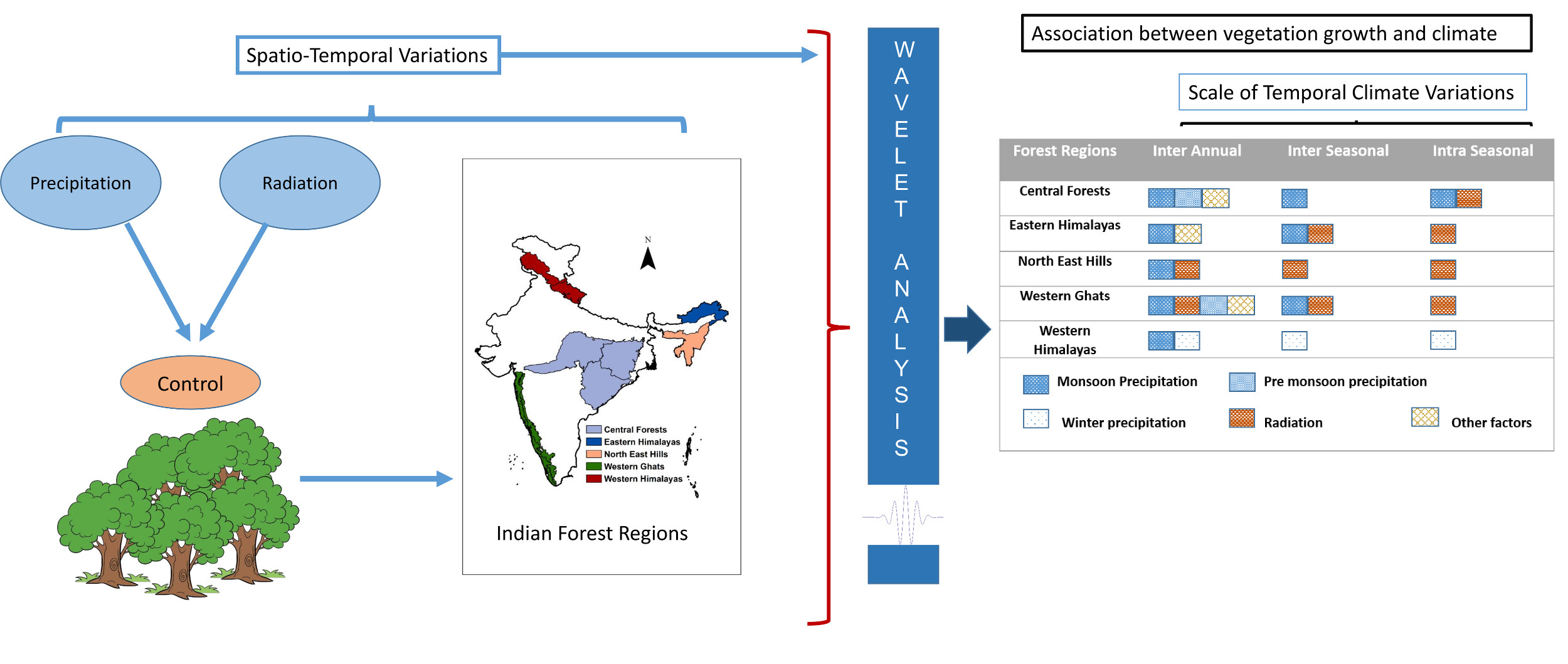
Figure 1. (a) The forested pixels, extracted based on the LULC map of Roy et al. (2015), considering deciduous broad-leaf forests, deciduous needle-leaf forests, evergreen broad-leaf forests, evergreen needle-leaf forests, mixed forests, and mangrove forests. (b) Classification of the forest pixels in India into five different forest regions based on the biogeographic zone classification by Rodgers et al. (2002).
Remotesensing 11 02703 g001
Figure 2. (a) Inter-annual variation of standard anomalies of enhanced vegetation index (EVI), precipitation, and radiation for the entire Indian landmass. (b) Inter-annual variation of standard anomalies of EVI, precipitation, and radiation considering only the forested pixels in India.
Remotesensing 11 02703 g002
Figure 3. Variation of EVI from the mean with precipitation and radiation anomalies (composites of positive and negative anomaly years), respectively for (a,b) central forests, (c,d) Eastern Himalayas, (e,f) northeast hills, (g,h) Western Ghats, and (i,j) Western Himalayas during the monsoon months (JJAS). The years with positive and negative anomalies in precipitation and radiation are considered separately to plot the composite EVI over such years with the variation among them represented by the colored band.
Remotesensing 11 02703 g003
Figure 4. The mean change in EVI between monsoon months (JJAS) and pre-monsoon months (MAM) denoted as delEVI.
Remotesensing 11 02703 g004
Figure 5. Spatial mean of multi-year averages of EVI (with the mean percentage of high quality MODIS EVI pixels at each step) (green curve), precipitation (blue curve), and radiation (yellow curve) values of the forest pixels for (a) central forests, (b) Eastern Himalayas, (c) northeast hills, (d) Western Ghats, and (e) Western Himalayas.
Remotesensing 11 02703 g005
Figure 6. Wavelet analysis: Power spectra of wavelet coherence between EVI and precipitation and the average coherence values for the study duration at different periodicities, respectively, for (a,b) central forests, (c,d) Eastern Himalayas, (e,f) Northeast hills, (g,h) Western Ghats, and (i,j) Western Himalayas.
Remotesensing 11 02703 g006
Figure 7. Wavelet analysis: Power spectra of wavelet coherence between EVI and radiation and the average coherence values for the study duration at different periodicities, respectively, for (a,b) central forests, (c,d) Eastern Himalayas, (e,f) Northeast hills, (g,h) Western Ghats, and (i,j) Western Himalayas.
Remotesensing 11 02703 g007
Table 1. Limiting variables in different forest regions at different temporal scales.
Forest RegionsInter AnnualInter SeasonalIntra Seasonal
Central Forests Remotesensing 11 02703 i001 Remotesensing 11 02703 i002 Remotesensing 11 02703 i003
Eastern Himalayas Remotesensing 11 02703 i004 Remotesensing 11 02703 i003 Remotesensing 11 02703 i005
North East Hills Remotesensing 11 02703 i003 Remotesensing 11 02703 i005 Remotesensing 11 02703 i005
Western Ghats Remotesensing 11 02703 i006 Remotesensing 11 02703 i003 Remotesensing 11 02703 i005
Western Himalayas Remotesensing 11 02703 i007 Remotesensing 11 02703 i008 Remotesensing 11 02703 i008
Remotesensing 11 02703 i002Monsoon Precipitation Remotesensing 11 02703 i009Pre monsoon precipitation
Remotesensing 11 02703 i008Winter precipitation Remotesensing 11 02703 i005Radiation
Remotesensing 11 02703 i010Other factors

