Abstract
On 17 November 2017, a Mw 6.5 earthquake occurred in Mainling County, Nyingchi City, China. The epicenter was located in the Namche Barwa region of the eastern Himalayan syntaxis. Here, we have derived coseismic deformation from Global Positioning System (GPS) data and ascending Sentinel-1A Synthetic Aperture Radar (SAR) data. Based on a joint inversion of the two datasets, we obtained the coseismic slip distribution along a curved, northeast trending, and high-angle (dip angle of 75°) thrust fault. Our results show that the seismic moment release was 7.49 × 10¹⁸ N∙m, corresponding to a moment magnitude of Mw 6.55. The maximum slip was 1.03 m and the main rupture zone extended to a 12 km depth. The earthquake may have been related to the release of strain accumulated during the subduction of the Indian plate beneath the Eurasian continent. We identified a high strain rate and low b-values around the epicentral area before the earthquake, indicating that the earthquake was nucleated under a high strain/stress state. The data indicate two regions, southwest and southeast to the epicenter (the eastern Main Himalaya Thrust and northern end of the Sagaing fault), which remain under high stress/strain conditions and pose a significant seismic hazard.
1. Introduction
At 22:34 (UTC) on November 17, 2017, a Mw 6.5 earthquake (epicenter of 29.75° N, 95.02° E) struck Mainling County, Nyingchi City, Tibet (herein referred to as the Mainling earthquake), with a focal depth of 10 km (Figure 1). The maximum intensity given by the China Earthquake Administration was VIII [1]. No casualties were reported, but more than 3000 buildings were damaged. According to the focal mechanism provided by the Global Centroid Moment Tensor (GCMT) Project, the earthquake was a thrust event that occurred in the northern part of the Namche Barwa region, along the NNW-trending Xixingla fault [2]. More than 4000 aftershocks were recorded within the first week of the mainshock, including 22 M > 3 aftershocks [3], the largest being M 4.3. Owing to the remote location and difficult accessibility of the Namche Barwa region, no clear surface rupture was identified [3]. Nevertheless, owing to the dense seismic network deployed in eastern Tibet and advances in space geodesy, the earthquake was recorded with sufficient data coverage and quality to study its rupture process, and to investigate the crustal deformation and seismic activity of the Namche Barwa region. These results provide new insights into the crust dynamics of the eastern Himalayan syntaxis.
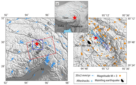
Figure 1.
Tectonic background of the 2017 Mw 6.5 Mainling earthquake. (a) Regional map showing the earthquake location. (b) Tectonic setting. Blue arrows indicate interseismic global positioning system (GPS) velocity fields of the eastern Himalayan syntaxis measured between 1999 and 2016 [1]; error ellipses indicate a 95% confidence level; the red rectangle marks the InSAR data coverage; the blue rectangle outlines the area shown in (c). (c) M > 3 earthquakes (orange dots) in the Namche Barwa region from 1965 to 2017 and aftershocks (blue dots) of the Mainling earthquake [10]. The beach ball indicates the Global Centroid Moment Tensor (GCMT) focal mechanism of the earthquake; the red star represents the epicenter; the blue line denotes the fault that likely generated the earthquake; black lines represent other faults in the study region [1] (JSZ: Jiali Shear Zone; DMF: Dongjiu-Mainling fault; NBS: Namche Barwa region; ZSF: Zayu fault; MAF: Motuo-Aniqiao fault; BLF: Baqing-Leiniaoqi fault; NJF: Nujiang fault; XXLF: Xixingla fault; IYSZ: Yarlung Zangbo suture zone; AS: Assam syntaxis).
Several studies have investigated the earthquake using finite fault modeling (Table 1) based on relocated aftershocks, interferometric synthetic aperture radar (InSAR) measurements, and teleseismic data [1,3,4,5,6,7,8]. However, there are inconsistencies among the different fault models, coseismic slip distributions, and produced Coulomb stress changes. For example, using teleseismic data and InSAR-measured surface deformation, Liu et al. [1] reported that the earthquake broke one asperity, and that ruptures were concentrated between the surface and at a 10 km depth, with a maximum slip of 0.51 m. However, Li et al. [9] identified two coseismic slip areas, dominantly distributed at depths of 5–15 km, with a maximum slip of 0.83 m. Based on the aftershock data, Xiong et al. [6] suggested that the earthquake ruptured two adjacent parallel faults. Their inversion results based on the InSAR data provide comparable maximum slips of 0.36 and 0.43 m on the two fault planes. In addition, the different studies have considered divergent fault plane solutions (Table 1), which has also resulted in ambiguities in slip modeling. All of these discrepancies are due to a lack of observations that can constrain the fault model well.

Table 1.
Source parameters of the 2017 Mw 6.5 Mainling earthquake.
In this study, we have included GPS displacement data for the first time. These data were acquired in campaign-mode before and after the earthquake. By referring to field geological survey data [11,12], we also determined a curved fault plane, according to the relocated aftershock distribution, and optimized the dip-angle according to the data fitting quality of the slip models. This paper is organized as follows. We first introduce the tectonic background of the Namche Barwa region (Section 2), then describe the data processing of the coseismic displacement field, including the processing schemes for the GPS and SAR data (Section 3). Section 4 describes how the fault parameters were determined and the slip modeling results were obtained. In Section 5, we discuss the two fault planes of the 2017 Mainling earthquake and the regional seismic hazard before and after the earthquake. Our conclusions are presented in Section 6.
2. Seismological Background
The 2017 Mw 6.5 Mainling earthquake occurred in the Namche Barwa region of the eastern Himalayan syntaxis. This area is highly deformed, owing to collision between the Indian and Eurasian plates which has occurred since 40 Ma ago [14]. Modern geodetic measurements (e.g., GPS) have revealed significant crustal deformation in the Tibetan Plateau. The Mani-Yushu-Xianshuihe fault marks the northern boundary and the upper crust rotates clockwise around the eastern Himalayan syntaxis [15,16,17,18]. Tectonic movements are distributed across many large active faults, including the Jiali fault, Nujiang fault, Aparon fault, NE-trending Motuo fault, Mainling fault, Aniqiao fault, and Yarlung Zangbo fault [19,20] (Figure 1). This region also suffers from severe surface erosion (5–17 mm/yr), accompanied by powerful fluvial activity (200 kW/m), heavy river incision, and intense rock metamorphism [21,22].
The eastern Himalayan syntaxis accommodates strong seismic activity. Aside from the 2017 Mainling earthquake, at least seven M > 7 large earthquakes have occurred here in the last century [1], including the 1947 M 7.7 Nang country earthquake, located 200 km southwest of the 2017 Mainling earthquake [22], and the 1950 M 8.6 Zayu earthquake, located approximately 220 km southeast of the Mainling event [23]. The Zayu earthquake was also followed by a series of M > 6 aftershocks. The 2017 Mw 6.5 Mainling earthquake, a high-angle thrust event, caused by the NE-dipping thrust of the Namche Barwa region subducting beneath the Lhasa terrane [1], broke a regional seismic quiescence that had lasted for over 50 years.
3. Geodetic Data
3.1. GPS Data
In order to study interseismic crustal deformation in the eastern Himalayan syntaxis, we deployed 13 GPS stations on the two sides of the Yarlung Zangbo River, near the Mainling epicenter, and conducted three repeated observations between 2015 and 2017. The day after the Mainling earthquake (18 November 2017), we conducted measurements at eight GPS sites located within 100 km of the epicenter and obtained position data from at least 24-h of continuous observations for each station.
The GPS Receiver Independent Exchange (RINEX) data, with a 30-sec sampling rate, were processed using the GAMIT/GLOBK 10.6 software [24]. The GPS carrier phase data were first processed to obtain loosely constrained daily solutions, along with the associated variance-covariance matrices. In this processing step, we adopted the latest absolute receiver antenna models of the International Global Navigation Satellite System (GNSS) Service (IGS), atmospheric zenith delay models [25], and the global mapping functions for the neutral atmosphere. Then, the loosely constrained daily solutions were transformed to a regional reference frame through combination with 20 IGS stations near the epicenter, after translation, rotation, and scaling using seven parameter transformations. Finally, coseismic displacements were estimated from these daily time series using the least squares method. The average measurement errors in the eastern and northern components were 2.85 and 2.69 mm, respectively. Table 2 provides the coseismic displacements of the eight GPS stations (Figure 2a). It is apparent that the deformation in the near field was larger than that in the far field, showing a rapid decay with distance from the fault, which suggests a rupture along a high-angle thrust fault. Although the postseismic effects in the first few days following the mainshock may be included in the estimated coseismic displacements, their magnitudes should be very small in comparison with the coseismic component and are thus negligible.

Table 2.
Coseismic global positioning system (GPS) displacements of the 2017 Mainling earthquake.
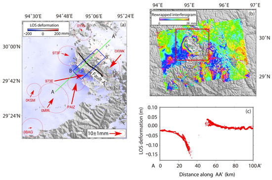
Figure 2.
Coseismic displacement data. (a) Global positioning system (GPS)-based displacements (red arrows); the black line marks the fault trace; error ellipses indicate a 95% confidence level; the blue rectangle indicates the aftershock region, used to demonstrate the along-depth distribution shown in Figure 3a; the green line displays the profile for plotting the line-of-sight (LOS) deformation shown in panel (c); (b) Rewrapped coseismic interferogram of the 2017 Mw 6.5 Mainling earthquake. The determined LOS deformation field outlined by the red rectangle is color-coded in panel (a); (c) LOS deformation of profile AA’, as marked in panel (a).
3.2. InSAR Data
We selected ascending frames from Sentinel-1A that were acquired 6 days before the earthquake (11 November 2017) and 6 days after the earthquake (23 November 2017) to reconstruct coseismic surface displacements. The SAR data were processed using the GAMMA software, following a standard single-pair differential interferogram generation strategy [26]. Topography effects were removed from the interferogram using the 90-m resolution Shuttle Radar Topography Mission (SRTM) digital elevation model (DEM). We used adaptive filtering to reduce the phase noise in the differential interferogram, and then used the minimum cost flow algorithm for phase unwrapping [27]. After geocoding, we obtained the line-of-sight (LOS) coseismic deformation field of the Mainling earthquake (Figure 2). The unwrapped coseismic deformation map (Figure 2a) shows negative LOS deformation (away from the satellite), with a maximum value of approximately 0.17 m occurring on the southwest side of the fault, and a positive LOS deformation (towards the satellite) with a maximum value of 0.05 m on the northeast side. However, the near-field interferogram (ascending) is decorrelated, owing to snow and vegetation coverage over the Namche Barwa region [11]. Satellite data (from Sentinel-2 and Landsat 8) after the earthquake also indicate widely distributed landslides, covering a large area near the fault, which further strengthens the decorrelation effect [1].
We extracted a displacement profile that passes through the earthquake epicenter and is normal to the fault (Figure 2c). This profile shows maximum LOS displacements of 0.14–0.15 m on the southwest side of the fault and 0.05 m on the northeast side, indicating a reverse faulting process. We acquired the SAR image 6 days after the earthquake, and thus, these displacements inevitably involve postseismic relaxation processes. However, we expect that early postseismic deformation, which is mainly attributed to afterslip and/or poroelastic relaxation, is concentrated in the near-field, where the interferogram loses coherence. Thus, postseismic relaxation does not significantly contribute to our determined coseismic displacements [28]. Since the complete InSAR data comprise millions of pixels, there is significant redundancy in constructing a source model from all observations. Therefore, we down-sampled the InSAR data based on the uniform sampling rule, using a 150-m resolution, while retaining deformation information. In total, we obtained 1365 observations.
4. Finite Fault Modeling
4.1. Fault Geometry
To obtain the coseismic slip of the 2017 Mainling earthquake, we first determined a fault model. Based on field geological investigations [11,12] and the relocated aftershock catalog [3], we outlined a curved fault trace comprised of three segments, namely, a northern segment with an average strike of 323°, a middle segment with a strike of 307°, and a southern segment with a strike of 319°. The fault has a length of 48 km, and we assumed that the fault reaches a depth of 30 km. During coseismic slip modeling, we discretized the fault plane into small patches of 3 × 3 km.
According to dislocation theory [29,30], a slip on a fault can be linearly projected to the ground surface by means of Green’s functions [31]. Therefore, with known coseismic displacements, we can invert for fault slip using the constrained least-squares algorithm on a fault plane with different dip angles. The optimization procedure was realized using a Steepest Descent Method (SDM) Program [32]. We evaluated the slip model according to the data-fitting quality measured by the root mean square (RMS).
The along-depth distribution of the relocated aftershocks (Figure 3a) were concentrated on the eastern side of the fault trace, suggesting that the fault plane likely dips to the east in a range marked by ‘OA’ and ‘OB’ in Figure 3a, corresponding to a dip angle between 60° and 85°. Therefore, we tested different dip angles in the range outlined by the aftershock distribution and identified an optimal dip angle of 75° to explain the surface displacements (Figure 3b). This value was used for slip modeling.

Figure 3.
Dip angle of the fault. (a) Aftershock (green dots) profile along profile BB’, marked in Figure 2a. O denotes the location of the fault trace; OA and OB outline the dominant aftershocks and imply the possible location of the fault plane. (b) Root mean square (RMS) values of the slip model as a function of the fault plane dip angle, where the red dot marks the optimal dip angle.
In the joint inversion of GPS and InSAR data, we also considered their relative weights, which were tested in the range of 1:0.1 to 1:20. An optimal ratio of 1:3.5 was found to best explain the entire geodetic dataset.
4.2. Checkerboard Test
To examine the geodetic data resolution for the slip distribution on the fault plane, we conducted three checkerboard tests, using GPS, InSAR, and both datasets. According to Wang et al. [33], we assigned synthetic slips of 0 and 1 m on different fault patches (Figure 4a), whose produced surface displacements were used for retrieving the slip on the fault (Figure 4b–d). We generated synthetic displacements for both the GPS stations and InSAR observation sites. These synthetic displacements include errors that follow a Gaussian distribution.
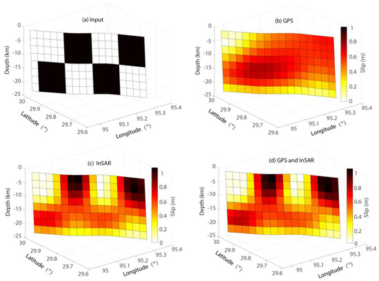
Figure 4.
Checkerboard test. (a) Input model, where black = 1 m and white = 0 m. Retrieved fault slip using (b) synthetic global positioning system (GPS) data only; (c) using synthetic interferometric synthetic aperture radar (InSAR) data only; (d) using both datasets.
The checkerboard test results show that the GPS network has a relatively poorer fault slip resolution compared with InSAR, owing to the sparse GPS site coverage (Figure 4b,c). The joint inversion based on both the GPS and InSAR data better resolves the fault slip, decreasing the modeling errors by 10% and 30% when compared with the results based only on the InSAR or GPS data, respectively. The modeling errors were evaluated according to the differences between the synthetic and inverted slips. Therefore, the GPS data play an important role in constructing the slip model of the 2017 Mainling earthquake. Overall, the available geodetic data have a relatively better resolution above the 12 km depth.
4.3. Modeling Results for the 2017 Mw 6.5 Mainling Earthquake
Figure 5 shows the modeling results for the 2017 Mainling earthquake. The inverted coseismic slip distribution (Figure 5a; fault slip data are provided in the supplementary materials) reveals one large slip patch, extending 30 km along the strike. The maximum slip (1.03 m) was located on the northern segment of the fault, near the surface. The slip model also indicates that the earthquake rupture reached the surface and was concentrated above a 12 km depth. The slip was mainly characterized by reverse faulting, consistent with the GCMT solution determined from the teleseismic data [1]. The determined coseismic slip is dominantly located in the zone where the geodetic observations have good resolution (according to the checkerboard test), suggesting that the slip is well constrained by the data. Assuming a shear modulus of 30 GPa, the determined slip model has a total moment of 7.49 × 10¹⁸ N∙m, corresponding to a moment magnitude of 6.55, which is close to the officially released value of Mw 6.5 [9].
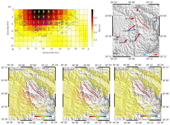
Figure 5.
Modeling results. (a) Coseismic slip distribution determined from both global positioning system (GPS) and interferometric synthetic aperture radar (InSAR) data; green arrows indicate slip directions. (b) Comparison between the observed (blue arrows) and modeled (red arrows) GPS data; lower panels show the (c) down-sampled InSAR data, (d) modeling result, and (e) their residuals. The red rectangles in panels b–e indicate the fault plane and the solid red line marks the fault trace.
This slip model fits well with the observed coseismic displacements, providing RMS values of 4.3 mm for the GPS data and 15.2 mm for the InSAR data. Comparisons between the observed and modeled displacement fields (Figure 5b–e) demonstrate small misfits overall, without systemic bias. Some large localized misfits could be related to heterogeneity that our elastic, half-space model could not account for.
As seen in Figure 5a, aftershocks were dominantly located around the coseismic rupture, where coseismic stress perturbation is expected to be high, owing to the strong slip gradient. The occurrence of aftershocks demonstrates one type of postseismic relaxation (beside afterslip, viscoelastic relaxation, and poroelastic rebound) in response to the coseismic stress perturbation.
We also tested the modeled coseismic slip from the GPS and InSAR data independently (Figure 6), and the results indicate that although the modeled slip based on each of these two data types is different from that of the joint inversion (Figure 5a), they share common features. This suggests that both InSAR and GPS data play important roles in constraining the coseismic slip distribution, with good consistency, despite the data being collected during slightly different time periods.
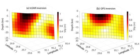
Figure 6.
Slip models. Models using (a) interferometric synthetic aperture radar (InSAR) data only and using (b) global positioning system (GPS) data only.
5. Discussion
Incorporating both the GPS and InSAR measured coseismic displacement data, including the relocated aftershocks, we constructed a slip model for the 2017 Mw 6.5 Mainling earthquake. The model can explain the geodetic data well, and, in general, the slip displays a disjointed distribution with the aftershocks. Using our results, we addressed two questions: (1) Was the secondary parallel fault involved in the coseismic rupture of the 2017 Mainling earthquake, as suggested by Xiong et al. [6]?; (2) What were the stress/strain conditions before and after the 2017 Mainling earthquake and what are the implications for regional seismic hazard?
5.1. Single-Plane Rupture or Double-Plane Rupture
Most studies have suggested that the Mainling earthquake ruptured a single fault [1,5,8], and this is consistent with our results. However, Xiong et al. [6] suggested that the Mainling earthquake ruptured two parallel faults [6], which are outlined by the aftershock distribution (Figure 1c and Figure 7). To investigate whether both fault planes were involved in the coseismic rupture of the 2017 Mainling earthquake, we investigated the spatiotemporal evolution of the relocated aftershocks (Figure 7). The results indicate that the aftershocks first occurred on the fault constructed in our coseismic slip model (Fault A). The first aftershock on the secondary parallel fault (Fault B) occurred 15 min after the mainshock. Both Fault A and Fault B belong to the Xixingla fault system [11,12]. The seismic moment release level along Fault B was higher in the later time period than that along Fault A. This temporal-spatial evolution of relocated aftershocks suggests that the aftershocks along Fault B were likely triggered by the coseismic rupture along Fault A.

Figure 7.
Early aftershocks. (a) Aftershocks within the first 15 min after the mainshock. (b) Aftershocks within the first hour after the mainshock. (c) Aftershocks within the first 7 days after the mainshock.
To further investigate the triggering effect, we calculated the coseismic Coulomb stress change, based on our slip model (Figure 5a), using the method of Scholz [34]:
where Δσc is the Coulomb stress change on the receiver fault, Δτs and Δσn represent changes in shear and normal stress (positive along the slip direction of the fault), respectively, and μ is the effective friction coefficient (ranging from 0 to 1) [34]. Using our slip model (Figure 5a), we considered a typical friction coefficient, μ, of 0.4 [35,36] and calculated Coulomb stress changes at 4, 8, and 12 km depths (Figure 8). The results indicate that Fault B is located in the zone of positive Coulomb stress change, and that the magnitude could be high enough to trigger earthquakes along Fault B.
Δσc = Δτs − μ(Δσn),
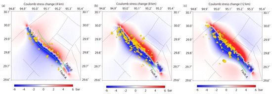
Figure 8.
Coulomb failure stress change based on the slip model in Figure 5a. Results for depths of (a) 4 km, (b) 8 km, and (c) 12 km. Yellow points denote aftershocks.
We also modeled the coseismic slip using two parallel fault planes (Figure 9). The double-plane model shows strong rupturing along Fault A, similar to that shown in Figure 5a, but a much weaker slip along Fault B. The results show that this model does not improve with the geodetic data fitting, where the residuals increased by 12.24% when compared with the one-fault model. On this basis, we conclude that Fault A played a dominant role during the 2017 Mw 6.5 Mainling earthquake, and that Fault B was, at most, marginally involved in the dynamic rupture.
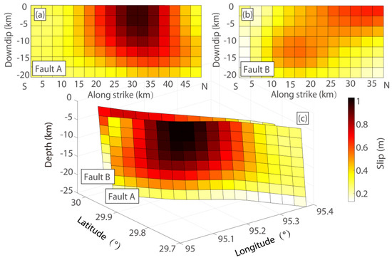
Figure 9.
Slip distribution along Fault A (a) and Fault B (b). (c) Overall view of the double-plane modeling results.
5.2. Stress/Strain State before and after the Mainling Earthquake
To understand the stress/strain state before and after the 2017 Mw 6.5 Mainling earthquake, we calculated the b-value from the regional seismicity and the strain rate from the long-term geodetic data. Then, we analyzed the impact of the earthquake on regional seismic hazard from the perspective of Coulomb stress change as shown in Figure 8.
The frequency-magnitude distribution of an earthquake usually follows the Gutenberg-Richter law:
where N is the number of earthquakes, equal to or greater than magnitude M, a reflects the seismic level of the target region, and b represents relative frequency of small and large earthquakes and has been thought to measure the variation of the stress in the crust [37]. Therefore, spatial/temporal variations of the b-value provide important insights into stress states relating to large earthquakes, and are important in seismic hazard assessment. Previous studies have shown that b-values in the epicentral area are small before the occurrence of a large earthquake [38,39,40,41]. For example, both the 2011 Mw 9.0 Tohoku and the 2004 Mw 9.1 Sumatra earthquakes were preceded by decreasing b-values in the main rupture zones [42]. Shi et al. [43] found that b-values decreased systematically before the 2008 Mw 7.9 Wenchuan earthquake.
log10N = a − bM,
For the 2017 Mw 6.5 Mainling earthquake, Han et al. [4] analyzed temporal variations in the b-value before the earthquake, however, they did not include spatial variations. In this study, we used a 50-year regional catalogue (from 1965 to the occurrence of the 2017 Mainling earthquake) [10] to map spatial variations in b-values [44]. According to the frequency-magnitude distribution, the complete magnitude in this region is approximately M 2.0. We used the ZMAP [45] to calculate b-values over a grid size of 0.2° × 0.2° (Figure 10a). The results show low b-values in the epicentral region prior to the Mainling earthquake, indicating a high stress state.
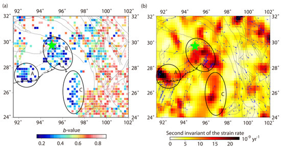
Figure 10.
Map view of b-value (a) and second invariant of the strain rate (b) before the Mainling earthquake. Blue arrows denote global positioning system (GPS)-derived displacement rates and the green star denotes the epicenter of the Mainling earthquake.
We also calculated the strain rate of the eastern Himalayan syntaxis, based on the long-term GPS displacement rates [46]. Using an L-curve method [47], we interpolated the GPS velocity field by 0.4° × 0.4° and calculated the second invariant of the strain rate tensor (effective strain rate), which characterizes the strain state of the upper crust [47]. The results indicate a high strain rate in the epicentral area (Figure 10b), which is consistent with the high stress conditions reflected in the b-values. Both the b-values and strain rate results suggest that the 2017 Mainling earthquake was nucleated under high stress/strain conditions. Furthermore, we identified two regions in the eastern Himalayan syntaxis, region A (along the eastern Himalaya Main Thrust) and region C (along the northern ends of the Sagaing fault), with high strain rates and low b-values. These regions pose a high seismic hazard. From the perspective of Coulomb stress change (Figure 8), we have found that the triggering effect of the Mainling earthquake was local. The earthquake imposed only very small stress perturbations on adjacent faults, and, as such, its impact on the regional seismic hazard was small.
6. Conclusions
In this study, we modeled GPS and InSAR displacement data for the 2017 Mw 6.5 Mainling earthquake. Incorporating the relocated aftershocks, we performed a joint inversion to determine the seismogenic fault plane and coseismic slip distribution. Based on our results, the earthquake occurred along a curved fault plane outlined by relocated aftershocks. The mainshock likely triggered a parallel fault plane, along which numerous aftershocks also occurred. The coseismic rupture extended 30 km along strike and 12 km downdip. The determined rupture reached the surface, with a maximum slip of 1.03 m. The earthquake released a total seismic moment of 7.49 × 10¹⁸ N∙m, corresponding to a magnitude of Mw 6.55. Using the interseismic GPS velocity field for 1999–2016 and the regional seismicity between 1965 and 2017, we calculated the second invariant of the strain rate and b-values of the eastern Himalayan syntaxis. The results demonstrate that the epicentral area of the 2017 Mw 6.5 Mainling earthquake, before its occurrence, had high strain rates and low b-values, indicating a high stress state. This suggests that the 2017 Mainling earthquake was nucleated under a high stress/strain state. Furthermore, the spatial distributions of strain rate and b-values show that zones along the eastern Himalaya Main Thrust and the northern end of the Sagaing fault remain under high stress and continue to pose a high seismic hazard.
Supplementary Materials
The following are available online at https://www.mdpi.com/2072-4292/11/24/2940/s1.
Author Contributions
Methodology, H.J., L.W., Y.L. (Yanchuan Li) and X.Y.; software, H.J., L.W., Y.L. (Yanchuan Li); validation, W.G. (Weijun Gan), S.L., Y.L. (Yanchuan Li), K.Z., Y.L. (Yunhua Liu), X.Y.; data curation, H.J., W.G. (Weijun Gan), S.L., Y.L. (Yanchuan Li), K.Z., Y.L. (Yunhua Liu), W.G. (Wenyu Gong), X.Y.; writing—original draft preparation, H.J.; writing—review and editing, H.J., L.W., W.G. (Wenyu Gong), S.L., Y.L. (Yanchuan Li), K.Z., Y.L. (Yunhua Liu), X.Y.; funding acquisition, L.W.
Funding
This work was supported by the National Natural Science Foundation of China (grant number 4167040536 and U1839211).
Acknowledgments
We are grateful to all of the staff involved in GPS data collection, to Sarah Henton De Angelis for the language revision, to ESA for providing Sentinel InSAR data (https://scihub.esa.int), to Wang Rongjiang for the SDM inversion program, and to Zhou Yijian for his assistance in the b-value calculation process. Figures were drawn using the GMT software (https://gmt.soest.hawaii.edu).
Conflicts of Interest
The authors declare no conflict of interest.
References
- Liu, Y.; Shan, X.; Zhang, Y.; Zhao, D.; Qu, C. Use of seismic waveforms and InSAR data for determination of the seismotectonics of the mainling Ms 6.9 earthquake on NOV.18, 2017. Seismol. Geol. 2018, 40, 79–100. [Google Scholar]
- Bai, L.; Li, G.; Song, B. The source parameters of the M 6.9 Mainling, Tibet earthquake and its tectonic implications. Chin. J. Geophys. 2017, 60, 4956–4963. (In Chinese) [Google Scholar]
- Yin, X.; Zhou, B.; Chen, J.; Wei, W.; Xie, C.; Guo, Z. Spatial-temporal distribution characteristics of early aftershocks following the M6.9 Mainling earthquake in Tibet, China. Chin. J. Geophys. 2018, 61, 2322–2331. (In Chinese) [Google Scholar]
- Han, J.; Yang, J.; Wang, W. Relocation of the aftershock sequence of Mainling Ms 6.9 earthquake in 2017 and spatio-temporal variation characteristics of b-value. Acta Seismol. Sin. 2019, 41, 169–180. [Google Scholar]
- Wei, W.; Xie, C.; Zhou, B.; Guo, Z.; Yin, X.; Li, B.; Wang, P. Location of the mainshock and aftershock sequences of the M 6.9 Mainling earthquake, Tibet. Chin. Sci. Bull. 2018, 63, 1493–1501. (In Chinese) [Google Scholar] [CrossRef]
- Xiong, W.; Chen, W.; Wen, Y.; Liu, G.; Nie, Z.; Qiao, X.; Xu, C. Insight into the 2017 Mainling Mw 6.5 earthquake: A complicated thrust event beneath the Namche Barwa syntaxis. Earth Planets Space 2019, 71, 71. [Google Scholar] [CrossRef]
- Hu, S.; Yao, H. Crustal velocity structure around the eastern Himalayan syntaxis: Implications for the nucleation mechanism of the 2017 Ms 6.9 Mainling earthquake and regional tectonics. Tectonophys 2018, 744, 1–9. [Google Scholar] [CrossRef]
- Wang, W.; Yang, J.; Wang, Y.; Jiang, X.; Zheng, Y. Imaging velocity structures and aftershock distributions in the source region of the 2017 Mainling M 6.9 earthquake. Chin. J. Geophys. 2019, 62, 2048–2058. (In Chinese) [Google Scholar]
- Li, W.; Xu, C.; Yi, L.; Wen, Y.; Zhang, X. Source parameters and seismogenic structure of the 2017 Mw 6.5 Mainling earthquake in the Eastern Himalayan Syntaxis (Tibet, China). J. Asian Earth Sci. 2019, 169, 130–138. [Google Scholar] [CrossRef]
- China Earthquake Datacenter. Available online: http://data.earthquake.cn/index.html (accessed on 6 October 2017).
- Xie, C. A Study on Tectonic Geomorphology of Namche Barwa and Activity of the Faults. Ph.D. Thesis, Institute of Geology, China Earthquake Adminstration, Beijing, China, 2019. (In Chinese). [Google Scholar]
- The 1:250000 Geological Map of Tibet Autonomous Region. Chengdu Inst. Geol. Miner. Resour. China 2003, 1. (In Chinese)
- Bai, L.; Li, G.; Khan, N.; Zhao, J.; Ding, L. Focal depths and mechanisms of shallow earthquakes in the Himalayan–Tibetan region. Gondwana Res. 2017, 41, 390–399. [Google Scholar] [CrossRef]
- Xu, Z.; Ji, S.; Cai, Z.; Zeng, L.; Geng, Q.; Cao, H. Kinematics and dynamics of the Namche Barwa Syntaxis, eastern Himalaya: Constraints from deformation, fabrics and geochronology. Gondwana Res. 2012, 21, 19–36. [Google Scholar] [CrossRef]
- Wang, Q.; Zhang, P.; Freymueller, J.; Bilham, R.; Larson, K.; Lai, X.; Liu, J. Present-day crustal deformation in China constrained by Global Positioning System Measurements. Science 2001, 294, 574–577. [Google Scholar] [CrossRef] [PubMed]
- Zhang, P.; Shen, Z.; Wang, M.; Gan, W.; Bürgmann, R.; Molnar, P.; Hanrong, S. Continuous deformation of the Tibetan Plateau from Global Positioning System data. Geology 2004, 32, 809–812. [Google Scholar] [CrossRef]
- Gan, W.; Zhang, P.; Shen, Z.; Niu, Z.; Wang, M.; Wan, Y.; Cheng, J. Present-day crustal motion within the Tibetan Plateau inferred from GPS measurements. J. Geophys. Res. 2007, 112–126. [Google Scholar] [CrossRef]
- Liang, S.; Gan, W.; Shen, C.; Xiao, G.; Liu, J.; Chen, W.; Zhou, D. Three-dimensional velocity field of present-day crustal motion of the Tibetan Plateau derived from GPS measurements. J. Geophys. Res. 2013, 118, 5722–5732. [Google Scholar] [CrossRef]
- Burg, J.; Nievergelt, P.; Oberli, F.; Seward, D.; Davy, P.; Maurin, J.; Diao, Z.; Meier, M. The Namche Barwa syntaxis: Evidence for exhumation related to compressional crustal folding. J. Asian Earth Sci. 1998, 16, 239–252. [Google Scholar] [CrossRef]
- Ding, L.; Kapp, P.; Wan, X. Paleocene–Eocene record of ophiolite obduction and initial India-Asia collision, south central Tibet. Tectonics 2005, 24, TC3001. [Google Scholar] [CrossRef]
- Tapponnier, P.; X, Z.; Roger, F.; Meyer, B.; Arnaud, N.; Wittlinger, G.; Yang, J. Oblique stepwise rise and growth of the Tibet Plateau. Science 2001, 294, 1671–1677. [Google Scholar] [CrossRef]
- Wang, P.; Scherler, D.; Liu-Zeng, J.; Mey, J.; Avouac, J.; Zhang, Y.; Shi, D. Tectonic control of Yarlung Tsangpo Gorge revealed by a buried canyon in Southern Tibet. Science 2014, 346, 978–981. [Google Scholar] [CrossRef]
- Chen, W.; Molnar, P. Seismic moments of major earthquakes and the average rate of slip in central Asia. J. Geophys. Res. 1977, 82, 2945–2969. [Google Scholar] [CrossRef]
- Herring, T.; King, R.; Floyd, M.; McClusky, S. GAMIT Reference Manual. GPS Analysis at MIT GLOBK, Release 10.6. Available online: http://www-gpsg.mit.edu/~simon/gtgk/GAMIT_Ref.pdf (accessed on 6 October 2017).
- Saastamoinen, J. Atmospheric Correction for the Troposphere and Stratosphere in Radio Ranging Satellites. Geophys. Monogr. Ser. 2013, 247–251. [Google Scholar]
- Werner, C.; Wegmüller, U.; Strozzi, T.; Wiesmann, A. Gamma SAR and interferometric processing software. In Proceedings of the Ers-Envisat Symposium, Gothenburg, Sweden, 16–20 October 2000; p. 1620. [Google Scholar]
- Werner, C.; Wegmüller, U.; Strozzi, T.; Wiesmann, A. Processing strategies for phase unwrapping for INSAR applications. In Proceedings of the European Conference on Synthetic Aperture Radar, Cologne, Germany, 4–6 June 2002; pp. 353–356. [Google Scholar]
- Shen, Z.; Sun, J.; Zhang, P.; Wan, Y.; Wang, M.; Bürgmann, R.; Zeng, Y.; Gan, W.; Liao, H.; Wang, Q. Slip maxima at fault junctions and rupturing of barriers during the 2008 Wenchuan earthquake. Nat. Geosci. 2009, 2, 718. [Google Scholar] [CrossRef]
- Ben-Menahem, A.; Singh, S. Multipolar elastic fields in a layered half space. Bull. Seismol. Soc. Am. 1968, 58, 1519–1572. [Google Scholar]
- Singh, S. Static deformation of a multilayered half-space by internal sources. J. Geophys. Res. 1970, 75, 3257–3263. [Google Scholar] [CrossRef]
- Okada, Y. Internal deformation due to shear and tensile faults in a half-space. Bull. Seismol. Soc. Am. 1992, 82, 1018–1040. [Google Scholar]
- Wang, R.; Diao, F.; Hoechner, A. SDM—A geodetic inversion code incorporating with layered crust structure and curved fault geometry. In Proceedings of the General Assembly European Geosciences Union, Vienna, Austria, 7–12 April 2013. [Google Scholar]
- Wang, L.; Hainzl, S.; Zöller, G.; Holschneider, M. Stress-and aftershock-constrained joint inversions for coseismic and postseismic slip applied to the 2004 M 6.0 Parkfield earthquake. J. Geophys. Res. 2012, 117, B07406. [Google Scholar] [CrossRef]
- Scholz, C. The Mechanics of Earthquakes and Faulting; Cambridge University Press: New York, NY, USA, 1990. [Google Scholar]
- King, G.; Stein, R.; Lin, J. Static stress changes and the triggering of earthquakes. Bull. Seismol. Soc. Am. 1994, 84. [Google Scholar]
- Yin, F.; Han, L.; Jiang, C.; Shi, Y. Interaction between the 2017 M 6.9 Mainling earthquake and the 1950 M 8.6 Zayu earthquake and their impacts on surrounding major active faults. Chin. J. Geophys. 2018, 61, 3185–3197. (In Chinese) [Google Scholar]
- Scholz, C. On the stress dependence of the earthquake b value. Geophys. Res. Lett. 2015, 42, 1399–1402. [Google Scholar] [CrossRef]
- Guha, S. Premonitory crustal deformations, strains and seismotectonic features (b-values) preceding Koyna earthquakes. Tectonophysics 1979, 52, 549–559. [Google Scholar] [CrossRef]
- Imoto, M. Changes in the magnitude—Frequency b-value prior to large (M ≥ 6.0) earthquakes in Japan. Tectonophysics 1991, 193, 311–325. [Google Scholar] [CrossRef]
- Molchan, G.; Kronrod, T.; Nekrasova, A. Immediate foreshocks: Time variation of the b-value. Phys. Earth Planet Inter. 1999, 111, 229–240. [Google Scholar] [CrossRef]
- Molchan, G.; Dmitrieva, O. Dynamics of the magnitude—frequency relation for foreshocks. Phys. Earth Planet Inter. 1990, 61, 99–112. [Google Scholar] [CrossRef]
- Nanjo, K.; Hirata, N.; Obara, K.; Kasahara, K. Decade-scale decrease in b value prior to the M 9-class 2011 Tohoku and 2004 Sumatra quakes. Geophys. Res. Lett. 2012, 39. [Google Scholar] [CrossRef]
- Shi, H.; Meng, L.; Zhang, X.; Chang, Y.; Yang, Z.; Xie, W.; Katsumi, H.; Han, P. Decrease in b value prior to the Wenchuan earthquake (Ms 8.0). Chin. J. Geophys. 2018, 61, 1874–1882. (In Chinese) [Google Scholar]
- Sreejith, K.; Sunil, P.; Agrawal, R.; Saji, A.; Rajawat, A.; Ramesh, D. Audit of stored strain energy and extent of future earthquake rupture in central Himalaya. Sci. Rep. 2018, 8, 16697. [Google Scholar] [CrossRef]
- Swiss Seismological Service. Available online: http://www.seismo.ethz.ch/en/research-and-teaching/products-software/software/ZMAP/ (accessed on 6 October 2017).
- Li, Y.; Shan, X.; Qu, C.; Liu, Y.; Han, N. Crustal deformation of the Altyn Tagh fault based on GPS. J. Geophys. Res. 2018, 123, 10309–10322. [Google Scholar] [CrossRef]
- Li, Y.; Shan, X.; Song, X.; Jiang, Y.; Gan, W.; Qu, C.; Wang, Z. Fault locking and slip rate deficit on the middle and southern segment of the Tancheng-Lujiang fault inverted from GPS data. Chin. J. Geophys. 2016, 59, 4022–4034. (In Chinese) [Google Scholar]
© 2019 by the authors. Licensee MDPI, Basel, Switzerland. This article is an open access article distributed under the terms and conditions of the Creative Commons Attribution (CC BY) license (http://creativecommons.org/licenses/by/4.0/).