Spatial and Temporal Variations of Particulate Organic Carbon Sinking Flux in Global Ocean from 2003 to 2018

Abstract

The monitoring of particulate organic carbon (POC) flux at the bottom of the euphotic layer in global ocean using remote sensing satellite data plays an important role in clarifying and evaluating the ocean carbon cycle. Based on the in situ POC flux data, this paper evaluated various estimation models. The global ocean POC flux from 2003 to 2018 was calculated using the optimal model, and its temporal and spatial variation characteristics were analyzed. In general, the annual average of global ocean POC flux is about 8.5–14.3 ${\mathrm{Gt}\mathrm{C}\mathrm{yr}}^{-1}$ for period of 2003–2018. In the spatial dimension, the POC flux in the mid-latitude ocean (30–60°) is higher than that in the low-latitude (0–30°). The POC flux in Continental Margins with water depth less than 2000 m accounted for 30% of global ocean, which should receive more attention in global carbon cycle research. In the time dimension, the global POC flux decreases year by year generally, but the POC flux abnormally decreases during El Niño and increases during La Niña. In addition, due to global warming, sea ice melting, and bipolar sea area expansion, POC flux in high-latitude oceans (60–90°) is increasing year by year.

1. Introduction

The ocean, an important carbon pool in the world [1,2], has absorbed about one-third of the carbon released by humans [3]. The transport process of carbon from the surface layer to the deep ocean mainly includes two processes, physics and biology, and the biological process is called Biological Carbon Pump (BCP) [4,5,6]. BCP plays an important regulatory role in global atmospheric carbon dioxide content and is also an important indicator of global carbon cycle research [7,8]. Current studies show the strength of BCP decline in response to the global climate change, resulting in the reduction of the ocean carbon storage and the increase of atmospheric ${\mathrm{CO}}_2$ [9,10]. Therefore, it has great significance to monitor the BCP’s efficiency accurately for understanding the global carbon cycle and the disturbance of anthropogenic carbon dioxide emissions [10]. BCP transfers carbon elements from the ocean surface to deeper layers through a series of biological processes. Among them, the vertical migration of particulate organic carbon (POC) plays an important role in this process. Some studies show the sinking flux of POC at the bottom of euphotic layer (POC flux) directly reflects the efficiency of BCP [11].

POC flux is the key to connecting the net primary productivity (NPP) and the seabed sedimentation carbon. Using solar energy and dissolved inorganic nutrients, phytoplankton absorb ${\mathrm{CO}}_2$ and convert it into POC, most of which is converted back to ${\mathrm{CO}}_2$ and released to the atmosphere when passes through consumers in the surface ocean, while only a little enters the deep sea water [12]. This process is involved in the deep sea water cycle, which directly leads to the reduction of carbon content in the surface sea water, thus promoting the exchange of ${\mathrm{CO}}_2$ at the air–sea interface. Therefore, one of the most important aspects of studying BCP is the measurement of POC flux. The methods for measuring POC flux in the field mainly include the sedimentation trap method [13] and radioisotope ${}_{}{}^{234}Th$ decay method [14]. Many researchers have studied POC flux in the Pacific Ocean, Indian Ocean, Atlantic Ocean, and other local sea areas based on these two POC flux measurement methods [15,16,17,18,19].

However, due to the high cost and the complex instrument operation of sedimentation trap method as well as the difficulties in chemical analysis by isotope method, field measurements are too sparse to analyze changes in POC flux at global scale and long time scale [20]. In order to better conduct research on POC flux, some numerical models have emerged, such as ecosystem models and earth system models [8,21,22]. Based on these models, researchers have carried out more in-depth research on the internal mechanism of POC flux and achieved significant results. The above measurement and modeling methods provide some effective ways to research the POC flux, while there are still some limitations. For example, to obtain continuous simulation data on a global scale requires a large amount of in situ and auxiliary data as input, which is often not easily accessible.

Remote sensing satellites have the characteristics of short revisit period and wide observation range, which can provide continuous observations of the global ocean. This technology provides a new way to estimate marine biomass and POC flux. The POC flux is linked directly with marine NPP by the ratio of “new productivity” to “total productivity” [23]. At present, a series of POC flux estimation models were proposed by using satellite remote sensing data (such as sea surface temperature, chlorophyll, euphotic layer depth etc.) [10,24,25,26,27,28]. Due to the limitations of satellites and the insufficiency of the research on sedimentation mechanism, the existing POC flux estimation models based on satellite remote sensing data are mainly empirical models with limited accuracy. However, the model results conform to the laws of marine ecology when expressing the seasonal variation of the POC flux, and so it is often used in the study of the temporal and spatial variation of global ocean POC flux [29]. More and more researchers are aware of the scientific benefits of using large-scale POC flux observations from satellite data [30].

There is no doubt that these remote sensing estimation models will facilitate the clarification of POC flux in ocean. Until now, there have been many studies on the spatiotemporal changes of POC flux based on remote sensing data [2,20,31,32,33]. For example, Stramska analyzed the seasonal and regional variability of POC flux in the Barents Sea from 1998 to 2014 using satellite observations [32]. However, most of these studies focus on local seas such as the Indian, Southern, and Pacific Oceans, and the analysis of large-scale and long time series of global ocean is insufficient. In addition, there is a lack of research on the internal relationship between changes in POC flux and other environmental parameters. Satellite data indicate a decrease in the global NPP [34,35,36], meaning that there is a negative trend in POC flux in global ocean. The decrease of POC flux could indicate that the BCP in the ocean is weakening, but these observations have not been effectively supported by time series data [37].

Therefore, this article conducts spatiotemporal analysis of POC flux over a long time series from 2003 to 2018. First, the accuracy of several classical POC flux estimation models and their applicability in different NPP data were evaluated by the in situ POC flux data. Then, the optimal model and the most suitable NPP were selected to obtain the global ocean monthly average POC flux from 2003 to 2018. After that, we discussed the temporal and spatial variations of global oceanic POC flux.

2. Materials and Methods

2.1. Remote Sensing Data

Moderate-resolution Imaging Spectroradiometer (MODIS) monthly products obtained from the Ocean Color Data (https://oceandata.sci.gsfc.nasa.gov/) are used as the input dataset, which include Sea Surface Temperature (SST), sea surface Chlorophyll (Chl), and euphotic zone depth (${\mathrm{Z}}_{\mathrm{eu}}$). The monthly ocean NPP data are provided by three different models: Vertically Generalized Production Model (VGPM) [38], Carbon based Production Model (CbPM) [39], and size-fractionated phytoplankton pigment absorption (aph) based Productivity Model (SAbPM) [40]. All products mentioned above are global-wide with the spatial resolution of 9 km from January 2003 to December 2018.

2.2. In Situ Data

The Joint Global Ocean Flux Research (JGOFS) was an international research program on the fluxes of carbon between the atmosphere and ocean, and within the ocean interior. It set up two time series stations in Hawaii (Hawaii Ocean Time series program (HOT), 22.8°N, 158.0°W: http://hahana.soest.hawaii.edu/hot/) and Bermuda (Bermuda Atlantic Time series Study (BATS), 31.7°N, 64.2°W: http://bats.bios.edu/), which can provide repeat measurements of POC flux at approximately monthly intervals by the sediment traps. In addition to these tropical in situ POC flux data from low-flux regions, in situ data of high-flux regions measured in the Beaufort Sea (71.3°3, 127.3°W) and East China Sea (30.4°4, 122.6°E) were also collected [41,42,43]. A total of 285 in situ POC flux samples from 2003 and 2016 were collected at different water depths. After data preprocessing, outlier removal and satellite synchronization matching, 230 POC flux data were used as the verification dataset, accounting for 80.7% of the original data.

2.3. POC Flux Estimation Models

The primary production in the oceans that results from allochthonous nutrient inputs to the euphotic zone is called “new production”, while the primary production that results from nutrient recycling in the surface waters is called “regenerated production”, total primary productivity is the sum of them [23]. Eppley et al. used a large number of measured data to prove that under the premise of stable marine productivity system, the output ratio of POC in the surface layer of the ocean is approximately equal to the ratio of new productivity to total productivity. Therefore, they proposed that the ratio of new productivity to total productivity is the “f-ratio”, which links ocean carbon cycle with ocean primary productivity obtained by remote sensing. In fact, the carbon of the upper ocean ecosystem should be stable and balanced from the perspective of long-term and large spatial scales, then the ratio of the POC flux to the total productivity (“e-ratio”) is substantially equal to “f-ratio” [26]. This makes the POC flux at the bottom of euphotic layer the product of “e-ratio’’ and NPP, as a result, many studies focus on the estimation of “e-ratio’’. Several classical models are listed in

Table 1. Several classical “e-ratio’’ estimation models.

Author	Model Expression
Baines (1994)	$e-ratio={10}^{-0.67+0.30\ast \log 10\left({\mathrm{chl}}_{\mathrm{tot}}/{\mathrm{Z}}_{\mathrm{eu}}\right)}$
Laws (2000)	$e-ratio=0.62-\left(0.02\ast \mathrm{SST}\right)$
Dunne (2005a)	$e-ratio=\max \left(0.04,\min \left(0.72,-0.0081\ast \mathrm{SST}+0.0668\ast \ln \left(\frac{\mathrm{Chl}}{{\mathrm{Z}}_{\mathrm{eu}}}\right)+0.426\right)\right)$
Dunne (2005b)	$e-ratio=\max \left(0.04,\min \left(0.72,-0.0101\ast \mathrm{SST}+0.0582\ast \ln \left(\frac{\mathrm{NPP}}{{\mathrm{Z}}_{\mathrm{eu}}}\right)+0.419\right)\right)$
Henson (2011) Laws (2011a) Laws (2011b)	$e-ratio=0.23{\ast \mathrm{e}}^{\left(-0.08\ast \mathrm{SST}\right)}$ $e-ratio=\frac{\left(0.5857-0.0165\ast SST\right)\ast NPP}{51.7+NPP}$ $e-ratio=0.04756\ast \left(0.78-\frac{0.43\ast \mathrm{SST}}{30}\right){\ast \mathrm{NPP}}^{0.307}$

, in which ${\mathrm{chl}}_{\mathrm{tot}}$ is the chlorophyll integral value in the euphotic zone and $Z_{eu}$ is the depth of ocean euphotic layer.

2.4. Methods for Model Comparison

The POC flux can be obtained by using these models mentioned above. However, the in situ POC flux data are measured at different water depths, so they cannot be compared directly. Establishing the relationship between POC fluxes at different depth are needed. Researchers have never stopped studying the vertical distribution of POC sedimentation: beginning from the POC sedimentation attenuation model proposed by Martin in 1987 [44], many researchers have studied the vertical distribution characteristics of POC flux [45,46,47,48,49]. However, Martin’s model is still deemed as a powerful model to estimate POC flux at different depths when analyzing large-scale POC flux. In this paper we used Martin’s model to compare the POC flux calculation results with the in situ POC flux and screen out the optimal estimation method. The formula is as follows:

$$\mathrm{POC}\left(\mathrm{z}\right)=\mathrm{POC}\left({\mathrm{z}}_0\right)\ast {\left(\frac{\mathrm{z}}{{\mathrm{z}}_0}\right)}^{-0.858}.$$

(1)

$\mathrm{POC}\left(\mathrm{z}\right)$ refers to the POC flux at the depth of z, ${\mathrm{z}}_0$ is the reference depth (for example, 150 m at HOT), and –0.858 is the flux attenuation coefficient.

By using the Martin’s model, we transformed all estimated POC flux into the equivalent value at the water depth of the in situ data. Based on these equivalent data, we evaluated the accuracy of the above POC flux models. The accuracy of the POC flux models can be assessed by using the following criteria: logarithmic deviation (Bias), logarithmic root mean square error (RMSD), and unbiased root mean square error (uRMSD) proposed by Friedrichs [50]. At the same time, the correlation coefficient (${\mathrm{R}}^2$) and the average relative error (r.e) were used to calculate the correlation and the average dispersion between the calculated results and the in situ data. The formulas for calculating the evaluation parameters are as follows:

$$\mathrm{Bias}=\overline{{\log }_{10}\left({\mathrm{POC}}_{\mathrm{m}}\right)}-\overline{{\log }_{10}\left({\mathrm{POC}}_{\mathrm{f}}\right)},$$

(2)

$$\mathrm{RMSD}={(\frac{1}{\mathrm{N}}{{\displaystyle \sum }}_{\mathrm{i}=1}^{\mathrm{N}}\left({\log }_{10}\left({\mathrm{POC}}_{\mathrm{m}}\left(\mathrm{i}\right)\right)-{\log }_{10}\left({\mathrm{POC}}_{\mathrm{f}}\left(\mathrm{i}\right)\right)\right))}^{1/2},$$

(3)

$$\mathrm{uRMSD}=\mathrm{sign}\left({\mathsf{\sigma }}_{\mathrm{m}}-{\mathsf{\sigma }}_{\mathrm{f}}\right)\times \sqrt{{\mathrm{RMSD}}^2-{\mathrm{Bias}}^2},$$

(4)

$${\mathrm{R}}^2=\frac{{{\displaystyle \sum }}^{}\left({\mathrm{POC}}_{\mathrm{m}}-\overline{{\mathrm{POC}}_{\mathrm{m}}}\right)\left({\mathrm{POC}}_{\mathrm{f}}-\overline{{\mathrm{POC}}_{\mathrm{f}}}\right)}{\sqrt{{{\displaystyle \sum }}^{}{\left({\mathrm{POC}}_{\mathrm{m}}-\overline{{\mathrm{POC}}_{\mathrm{m}}}\right)}^2}\sqrt{{{\displaystyle \sum }}^{}{\left({\mathrm{POC}}_{\mathrm{f}}-\overline{{\mathrm{POC}}_{\mathrm{f}}}\right)}^2}},$$

(5)

$$\mathrm{r}.\mathrm{e}=\frac{\overline{\left|{\mathrm{POC}}_{\mathrm{m}}-{\mathrm{POC}}_{\mathrm{f}}\right|}}{\overline{{\mathrm{POC}}_{\mathrm{f}}}},$$

(6)

where N is the number of sampled data, ${\mathrm{POC}}_{\mathrm{m}}$ is the POC flux obtained by the model, and ${\mathrm{POC}}_{\mathrm{f}}$ is the in situ POC flux. ${\mathsf{\sigma }}_{\mathrm{m}}$ and ${\mathsf{\sigma }}_{\mathrm{f}}$ are the logarithmic standard deviations of ${\log }_{10}\left({\mathrm{POC}}_{\mathrm{m}}\right)$ and ${\log }_{10}\left({\mathrm{POC}}_{\mathrm{f}}\right)$.

3. Results

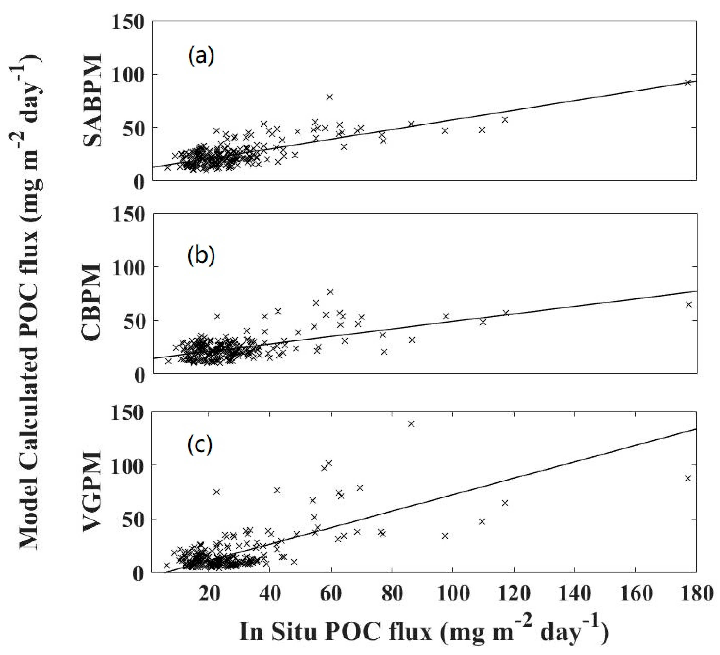
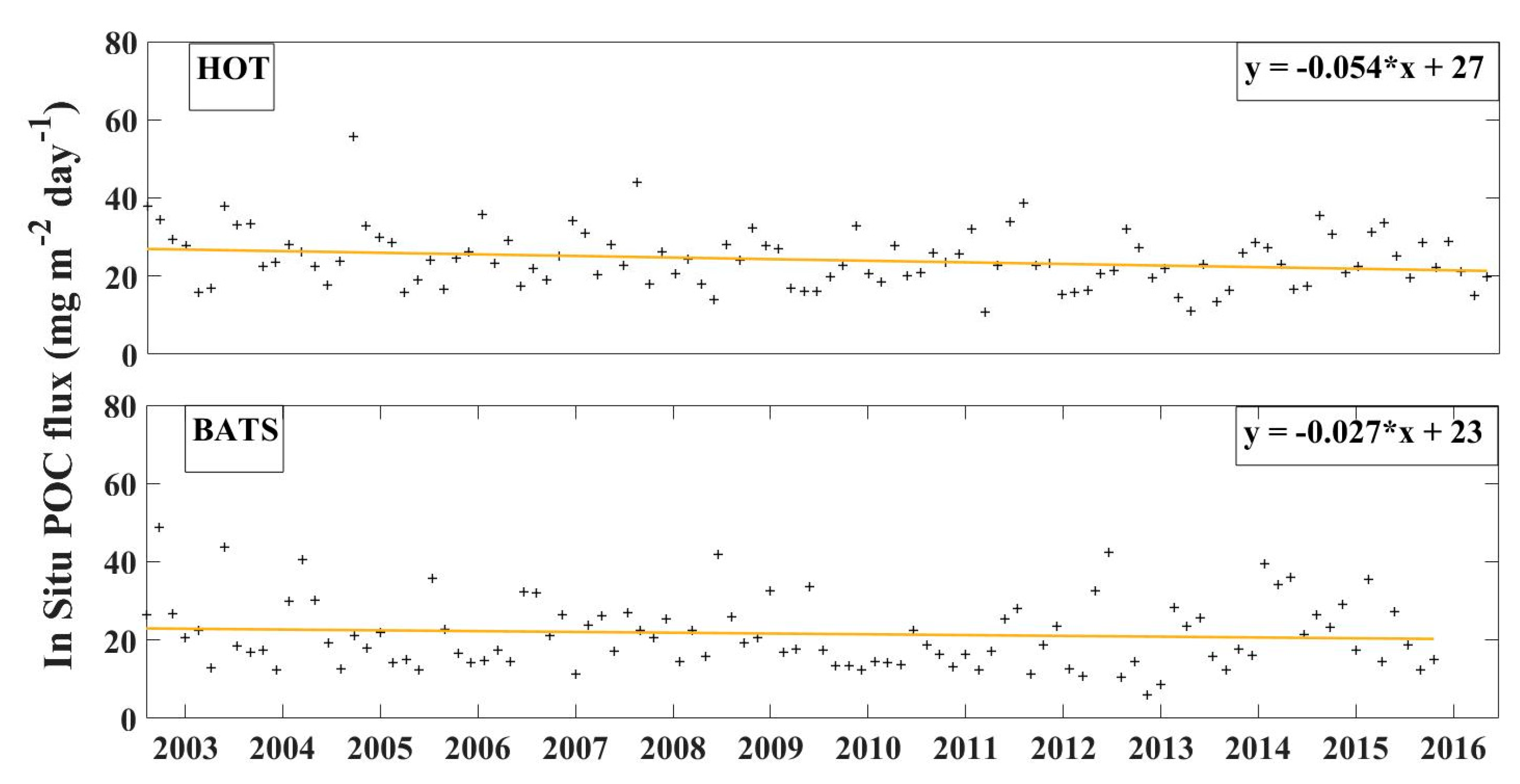
3.1. Evaluation of POC Flux Estimation Models

Common methods for calculating POC flux is to multiply e-ratio and NPP (Equation (7)). The accuracy of the global POC flux is determined by both e-ratio models and different NPP products.

$$\mathrm{POC}\mathrm{flux}=e-ratio\ast \mathrm{NPP}.$$

(7)

In this paper, we used seven classic e-ratio estimation models listed in Table 1 and three types of NPP products from SAbPM, VGPM, and CbPM to examine the accuracy and stability of different POC flux estimation models, and then chose the best combination for our research. There are three main steps involved: (1) calculating POC flux separately by using different e-ratio models based on remote-sensing derived parameters; (2) converting the calculated POC flux from step 1 to the data with the same water depth of in situ data by using Martin’s model; (3) comparing the converted POC flux (step 2) with the in situ data using Equations (2)–(6).

Table 2. Accuracy evaluation of different e-ratio models using different net primary productivity (NPP) products.

NPP Model	e-ratio Model	Bias	RMSD	uRMSD	R2	r.e
SAbPM	Baines (1994)	0.25	0.33	−0.21	0.01	0.84
	Laws (2000)	0.30	0.36	−0.19	0.31	0.97
	Dunne (2005a)	−0.01	0.17	−0.17	0.50	0.30
	Dunne (2005b)	0.24	0.31	−0.19	0.22	0.78
	Henson (2011)	−0.27	0.31	−0.16	0.33	0.50
	Laws (2011a)	0.42	0.45	−0.18	0.16	1.40
	Laws (2011b)	0.33	0.39	−0.21	0.01	0.84
CbPM	Baines (1994)	0.24	0.34	−0.24	0.09	0.88
	Laws (2000)	0.30	0.37	−0.23	0.23	1.02
	Dunne (2005a)	−0.02	0.19	−0.18	0.42	0.34
	Dunne (2005b)	0.23	0.33	0.24	0.14	0.85
	Henson (2011)	−0.28	0.35	−0.21	0.22	0.50
	Laws (2011a)	0.41	0.46	−0.22	0.10	1.48
	Laws (2011b)	0.32	0.41	−0.26	0.01	1.20
VGPM	Baines (1994)	−0.01	0.17	−0.17	0.45	0.32
	Laws (2000)	0.05	0.26	0.26	0.41	0.54
	Dunne (2005a)	−0.26	0.36	0.25	0.47	0.48
	Dunne (2005b)	−0.18	0.34	0.29	0.44	0.48
	Henson (2011)	−0.52	0.56	0.20	0.39	0.69
	Laws (2011a)	0.13	0.25	0.21	0.42	0.54
	Laws (2011b)	0.01	0.18	−0.18	0.42	0.34

lists the error evaluation results of different models using different NPP products. From Table 2, we can see Dunne (2005a) model using NPP data from SAbPM and CbPM models have higher accuracy than other e-ratio models using the same two NPP models, while the accuracy of Dunne (2005a) model using SAbPM is better. Although e-ratio models of Baines (1994) and Laws (2011a and 2011b) outperformed the Dunne (2005a) model by using NPP data from VGPM, the accuracy of these e-ratio models are much worse if using NPP data from SAbPM and CbPM models. Therefore, we figured out that e-ratio models of Dunne (2005a) combined with NPP from SAbPM have better stability and accuracy.

As the in situ data of high-flux regions are collected from different water depths, some of them are much higher than POC flux in low-flux regions. In order to better reflect the relationship between the in situ POC flux and the estimated results both in high and low flux regions, we converted the in situ data and the inversion data in high-flux regions into the data at the water depth of 150 m based on Martin’s model. Then, Figure 1 was plotted to depict the performance of Dunne (2005a) e-ratio model by using different NPP models. It can be seen that the POC flux calculated with SAbPM is closer to the in situ data, with the minimum dispersion and the highest correlation, which is consistent with the error calculation results (${\mathrm{R}}^2$ is 0.50 and r.e is 30%) in Table 2.

Based on the analysis above, we chose the Dunne (2005a) e-ratio model and NPP product from SAbPM model to calculate the global monthly average POC flux. Although its average relative error is 30%, which cannot satisfy the detailed study of POC flux, it is good enough to analyze the spatial and temporal characteristics of global ocean POC flux [51].

3.2. Inversion Results of POC Flux

There are two main steps involved in calculating the POC flux in our research:

(1) Calculating the global oceanic POC output ratio (namely e-ratio) at the bottom of the ocean euphotic layer using the Dunne (2005a) e-ratio model and the monthly average Chl, SST, and ${\mathrm{Z}}_{\mathrm{eu}}$ product spanning from 2003 to 2018 (download from https://oceandata.sci.gsfc.nasa.gov/);

(2) Calculating the global monthly POC flux by multiply the e-ratio value and NPP from the SAbPM model (http://geodoi.ac.cn/WebCn/doi.aspx?Id=1280).

Figure 2 is the spatial distribution of the global average e-ratio at the bottom of euphotic layer from 2003 to 2018. From it we can see that the e-ratio is less than 0.1 in the low-latitude ocean, while the e-ratio is higher than 0.3 in the high-latitude ocean. The e-ratio in coastal ocean is generally larger than that in deep ocean.

Figure 3 depicts the spatial distribution of the annual average POC flux from 2003 to 2018. It can be seen that global annual POC flux has different distribution characteristics at different latitudes: annual average POC flux in the low-latitude ocean near the equator is below 30 g C per square meter per year, while POC flux of the ocean above 45° in both hemispheres is as high as 70 g C per square meter per year, or even more than 100 in continental costal ocean.

According to our estimates, the global average annual POC flux is approximately 11 Gt C per year, which is close to the estimated results of most models except from Henson and Lutz (

Table 3. Annual average of global total POC flux in several models.

Estimated Sources	Global Total POC Flux (Gt C yr−1)	Instructions
The result of this paper	8.5–14.3	Dunne (2005a)
Laws et al., 2000	11.1–12.9	Empirical algorithm of SST
Gnanadesikan et al., 2004	8.7–10	OCMIP2 PRINCE1
Schlitzer et al., 2002	9.6	Nutrient inversion
Bopp et al., 2001	9.5–13.1	COAM mode
Moore et al.,2002	7.9–12.0	COAM(NCAR) mode
Henson et al.,2011	4	Empirical algorithm of SST
Laws et al., 2011a	13.24	Algorithm of SST and NPP
Laws et al., 2011b	9.23	Algorithm of SST and NPP
Henson et al., 2015	8.5	Biogeochemical model
Laufkötter et al., 2016	7.7	Marine ecosystem models

) [10,26,27,52,53]. Considering the relative error of the model (30%, in Table 2), the range of the annual average is between 8.5 and 14.3 Gt C per year.

The entry of POC into deep seawater directly leads to a reduction in the carbon content of surface seawater, which further regulates the ${\mathrm{CO}}_2$ flux and promotes the exchange of ${\mathrm{CO}}_2$ at the air–sea interface [12]. Thence, we also conducted research on the spatial distribution of global sedimentation of organic carbon at ocean bottom (${\mathrm{F}}_{\mathrm{POC}}$). First, we obtained global ocean depth data (https://www.bodc.ac.uk/) with a spatial resolution of 1 rad from the British Ocean Data Center (BODC) and resampled it to 9 km. Then based on the global POC flux data, the global ocean depth data and Martin’s model, ${\mathrm{F}}_{\mathrm{POC}}$ from 2003 to 2018 were acquired (shown in Figure 4). From Figure 4, we can see the deposition flux of organic carbon in offshore seabed is obviously higher than that in deep ocean.

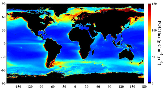
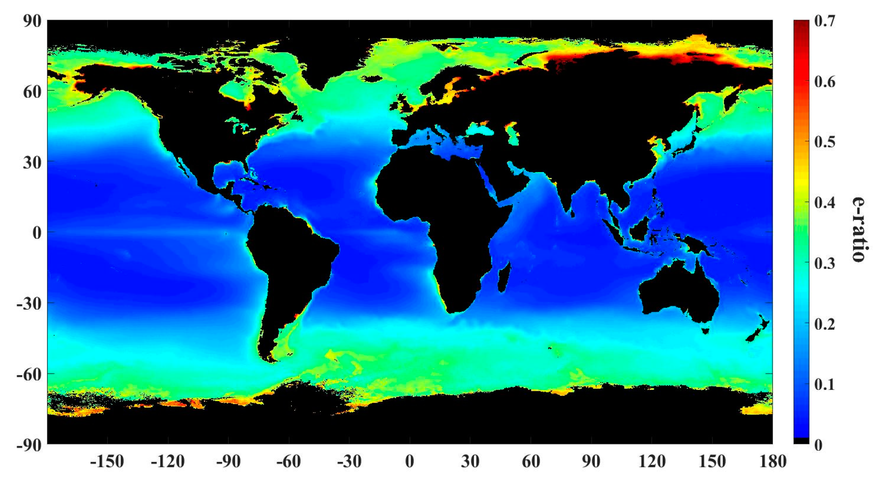
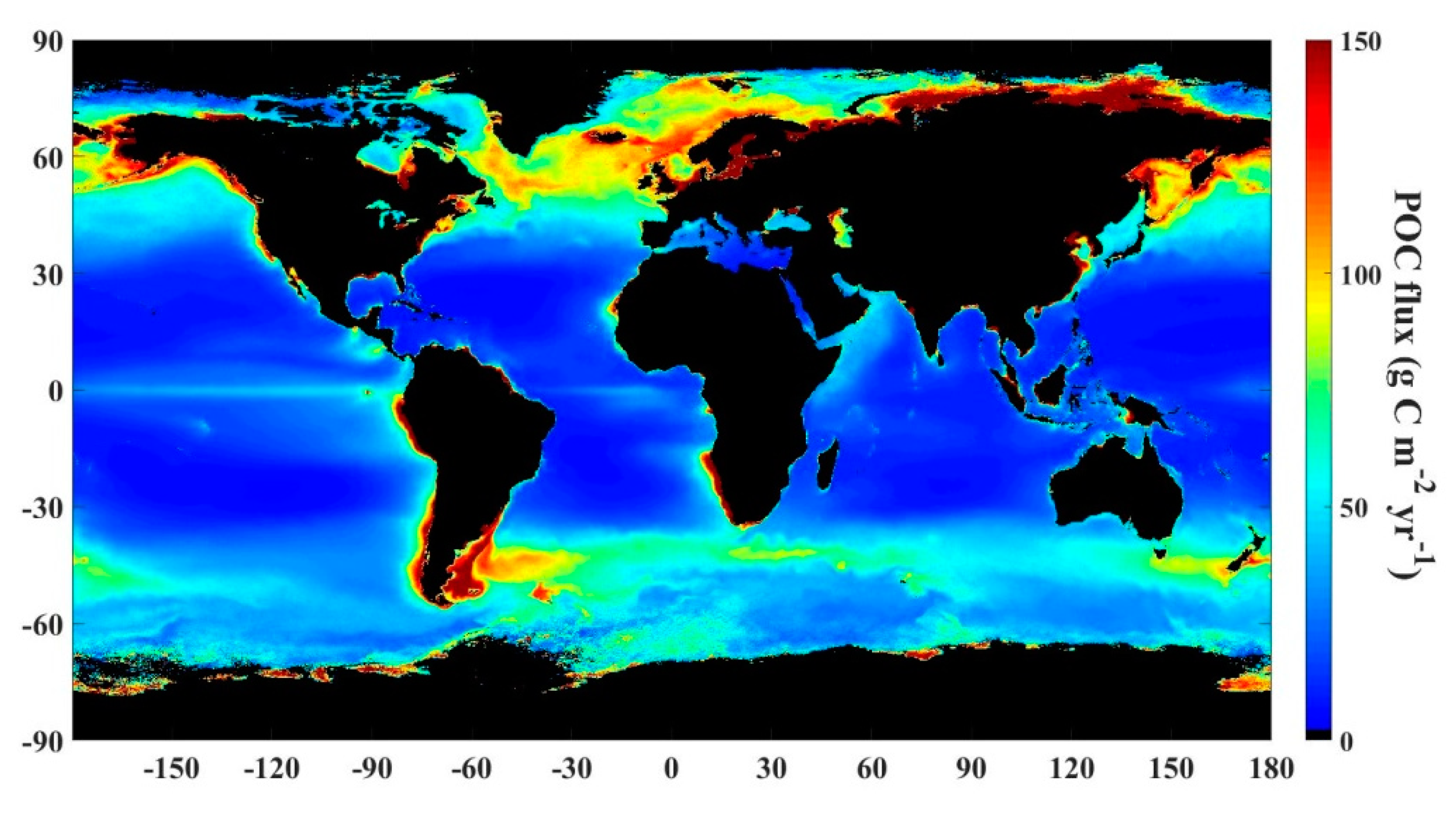
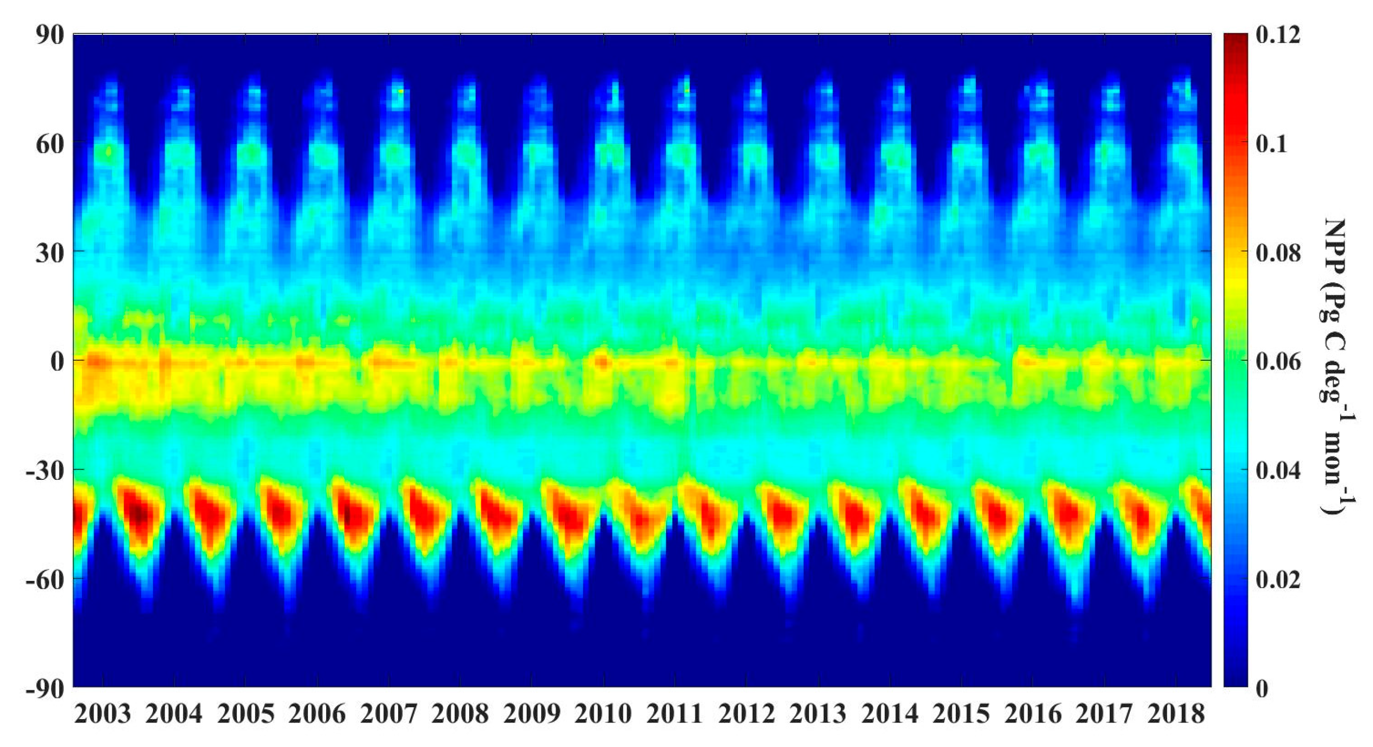
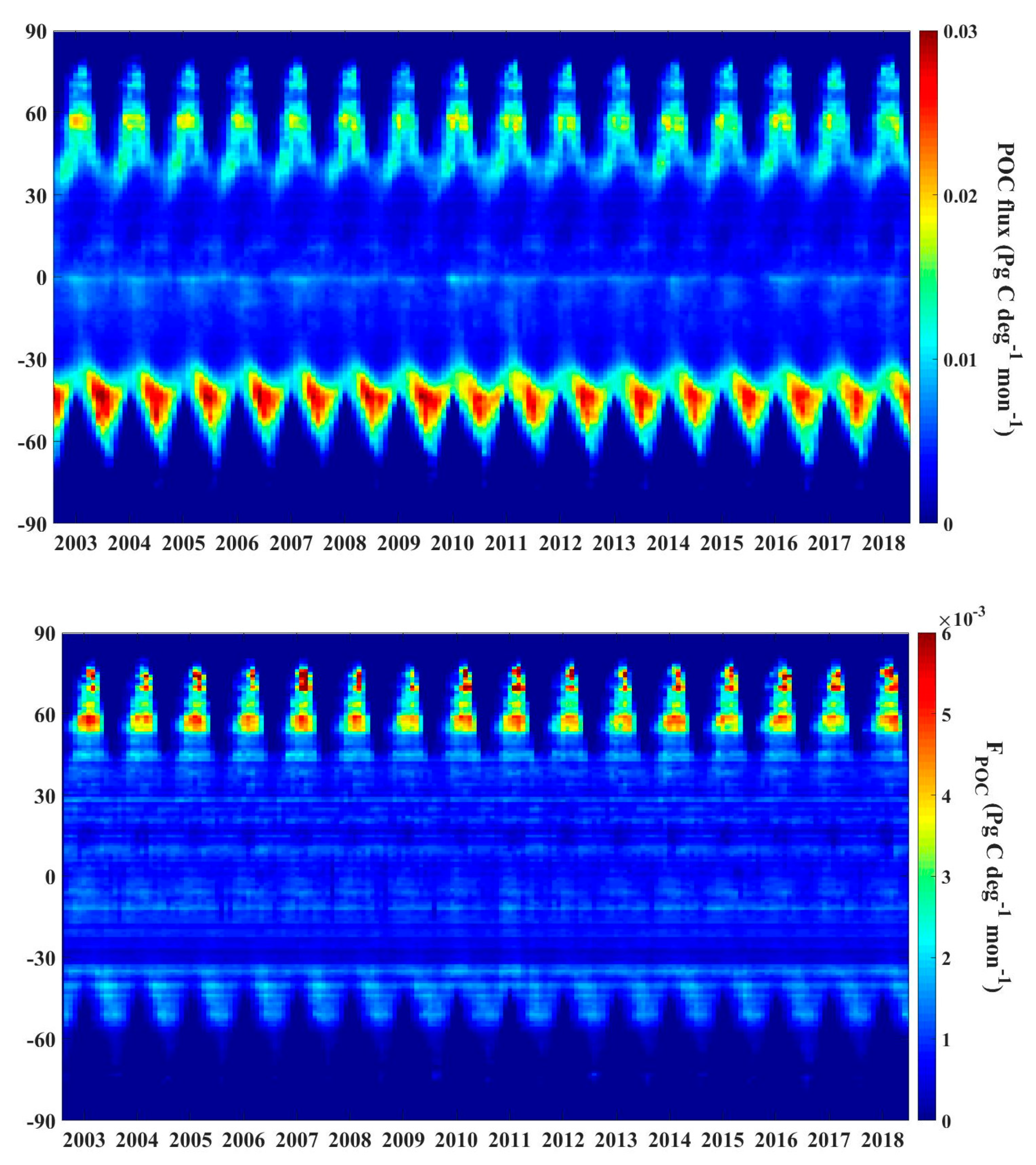
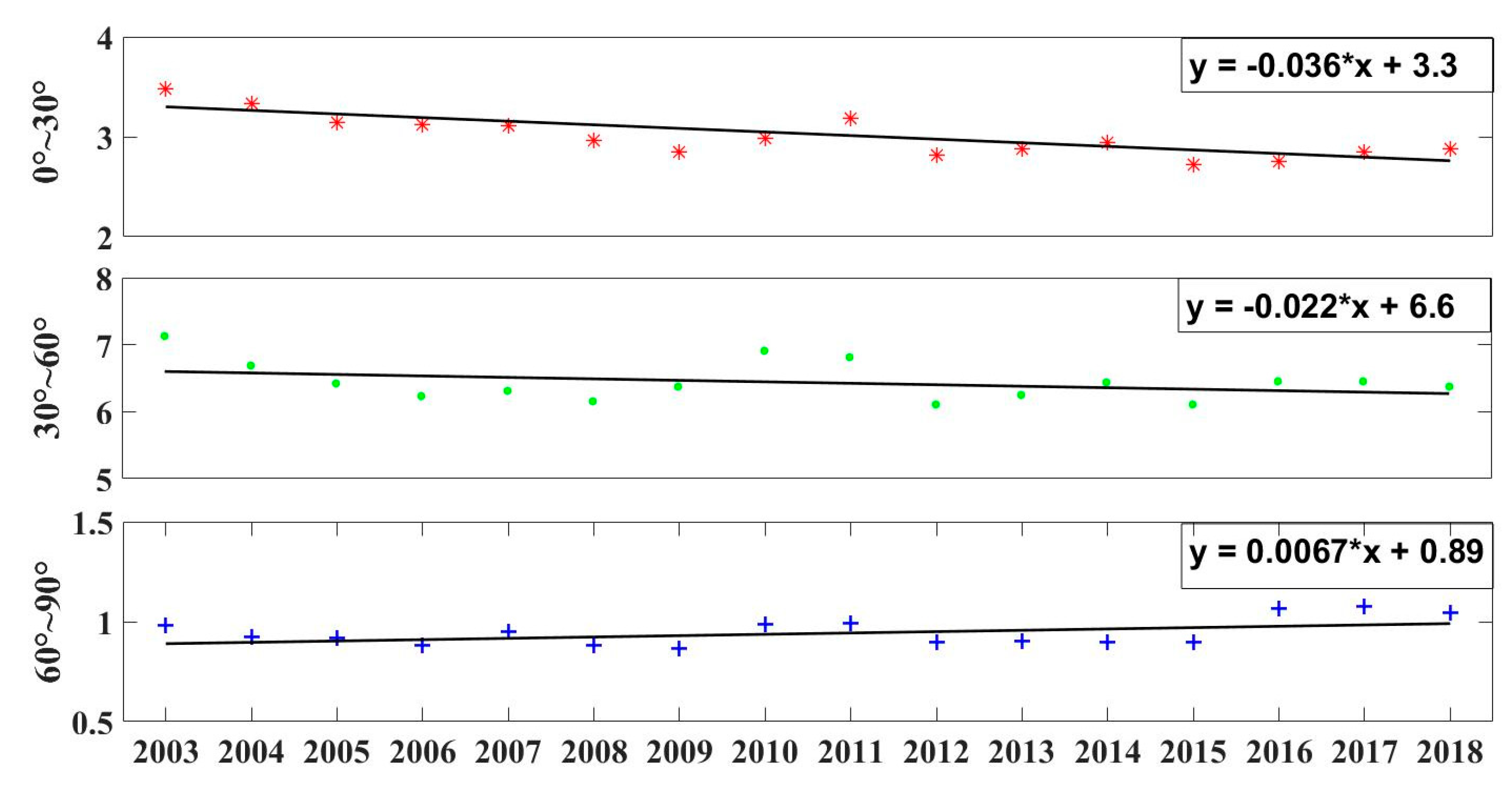
3.3. Spatial and Temporal Variations of POC Flux

In order to explore the spatial and temporal distribution of total NPP, POC flux, and ${\mathrm{F}}_{\mathrm{POC}}$, we calculated the integration of each monthly parameter respectively over each 1° latitude band from 2003 to 2018. The spatial and temporal variations distribution map of three parameters with latitude as y-axis and time as x-axis are depicted in Figure 5.

3.3.1. Spatial Variation

From Figure 5 we can see the POC flux and NPP show very similar spatial distribution characteristics. Both NPP and POC flux have peaks in the northern and southern hemispheres, but the peak in the southern hemisphere is significantly higher than that in the northern hemisphere. The high peak of POC flux in the region of 40–50°S can be attributed to high value of NPP formed by the westerly drift, high value of e-ratio, and also the large proportion of ocean area in the southern hemisphere and so on. In addition, the POC flux and NPP in both hemispheres show obviously seasonal variation due to the sun’s direct point moving back and forth between the north and south tropics. For example, in the winter, POC flux and NPP are at their low peaks in the northern hemisphere while POC flux and NPP are at their high peaks in the southern hemisphere, which is bathed in summer sunlight and heat. From Figure 5 we also found that although the high temperature and high humidity of the equatorial sea lead to a relatively higher NPP value, the total POC flux is significantly lower due to the low e-ratio in the low-latitude ocean (30°S–30°N), which accounts for only 30%–50% of POC flux in the mid-latitude ocean.

In order to further explore the spatial distribution characteristics of these parameters, we divided the world into several regions from two perspectives: six regions according to latitude (low-latitude (0–30°), mid-latitude (30–60°), and high-latitude (60–90°) in different hemispheres, respectively) and two regions according to depth of ocean (Continental Margins and Deep Ocean). In this paper, we divided water depth <= 2000 m as the Continental Margins (total area is about $4.8\times {10}^7{\mathrm{km}}^2$) and the water depth >2000 m as the Deep Ocean (total area is about $31\times {10}^7{\mathrm{km}}^2$) according to the classification criteria of Liu and Muller-Karger [54,55,56].

Table 4. Proportion of NPP, e-ratio, POC flux, and ${\mathrm{F}}_{\mathrm{POC}}$ distribution in different latitudes/oceans.

Region	NPP	e-ratio	POC Flux	FPOC
>60°N	3.3%	7.14%	8.7%	14.6%
30–60°N	15.2%	23.6%	24.0%	25.1%
0–30°N	25.3%	11.8%	12.7%	24.1%
0–30°S	30.4%	14.6%	16.0%	20.0%
30–60°S	25.4%	40.0%	37.0%	15.4%
>60°S	0.7%	2.7%	1.5%	0.4%
Continental Margins	18.1%	22.9%	29.5%	90.1%
Deep Ocean	81.9%	77.1%	70.5%	9.9%
Total	64.4 Pg m−2 yr1	———	11 Pg C m−2 yr−1	1.2 Pg C m−2 yr−1

presents the statistics about the proportion of NPP, POC, and ${\mathrm{F}}_{\mathrm{POC}}$ in different regions.

From Table 4, we found that the percentage of NPP at low-latitude accounts for about 56% due to the sufficient illumination and vast sea area, while POC flux in the same region only accounts for 28.7% owing to the low e-ratio. The total NPP (25.4%) and POC flux (37.0%) in the mid-latitude ocean in the southern hemisphere are higher than those in the northern hemisphere, which can be attributed to the lager sea area in the southern hemisphere. In the high-latitude ocean, the percentage of NPP and POC flux are quite low, accounting for only 4% and 10%, due to the limitation of illumination conditions and smaller ocean area. Though the NPP and POC flux in Deep Ocean account for 81.9% and 70.5% respectively, the proportion of NPP and POC flux in the Continental Margins are also important enough (18.1% and 29.5%).

When POC settles to the bottom of the ocean, the change of ${\mathrm{F}}_{\mathrm{POC}}$ between different latitudes is not obvious except for the middle and high latitudes in the northern hemisphere (Figure 5). As shown in Table 4, the percentages of ${\mathrm{F}}_{\mathrm{POC}}$ in the northern hemisphere in generally higher than that in the southern hemisphere and this pattern is particularly evident in high latitudes. The percentages of ${\mathrm{F}}_{\mathrm{POC}}$ in the high-latitude ocean of the northern and southern hemisphere are 14.6% and 0.4%, respectively. For the Continental Margins, the proportion of ${\mathrm{F}}_{\mathrm{POC}}$ is very high (over 90%) due to the shallower water depth and higher POC flux, while in the Deep Ocean, deeper sea depth and longer sedimentation period greatly reduce the proportion of ${\mathrm{F}}_{\mathrm{POC}}$ (less than 10%).

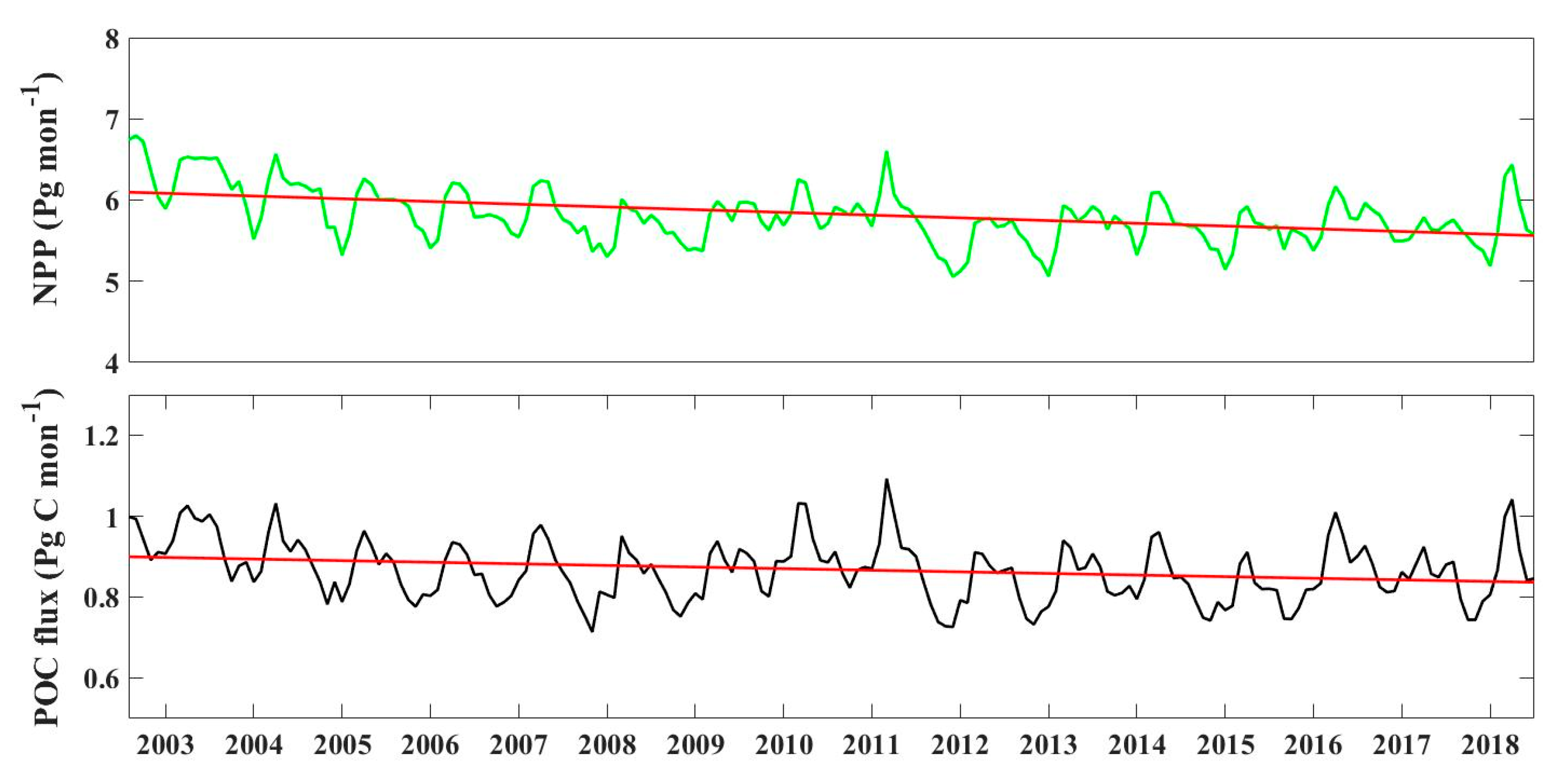
3.3.2. Temporal Variation

From Figure 5 we can observe not only the spatial but also the temporal distribution characteristics of NPP, POC flux, and ${\mathrm{F}}_{\mathrm{POC}}$. NPP and POC flux show a downward trend overall, especially after 2008. For example, from 2003 to 2018 the NPP in the equatorial sea area is reduced from 0.1 ${\mathrm{Pg}\mathrm{C}\mathrm{deg}}^{-1} mo{n}^{-1}$ to 0.07 or even lower, and the peak’s color of NPP in the southern hemisphere also becomes shallower from deep red which represents 0.12 ${\mathrm{Pg}\mathrm{C}\mathrm{deg}}^{-1}mo{n}^{-1}$. Unlike NPP, the POC flux shows a significant downward trend in the mid-high latitude ocean of both two hemispheres. From 2003 to 2018, the peaks of POC flux in the southern hemisphere decline from 0.03 ${\mathrm{Pg}\mathrm{C}\mathrm{deg}}^{-1} mo{n}^{-1}$ to about 0.025, while peaks in the northern hemisphere decrease from 0.02 to about 0.015. Due to the very low e-ratio in the equatorial ocean, the difference of POC flux in the equatorial region is not obvious. As for the ${\mathrm{F}}_{\mathrm{POC}}$, the slowness of the sedimentation process and the long period of the deep-sea change (hundred years) make the inter-annual variation of ${\mathrm{F}}_{\mathrm{POC}}$ very weak [57]. Therefore, we cannot observe the obvious change of ${\mathrm{F}}_{\mathrm{POC}}$.

Figure 6 is the trend graph for global NPP and POC flux from 2003 to 2018. In this figure, the monthly NPP and POC flux shows an overall decreasing trend. The slope of the NPP trend line is –0.0028, while the POC flux’s is –0.00033. Therefore, we determined that the POC flux is decreasing slower than NPP which can be attributed to the low e-ratio (less than 0.7). Although the general trend of POC flux is declining year by year, there are some abnormal years. For example, the black line in Figure 6 has many abnormal bulges, which is much higher than the trend line. In particular, the monthly total POC flux increased abnormally during 2010–2011 and 2016–2017.

4. Discussion

4.1. POC Flux in Continental Margins

Compared with the open oceans, the biological productivity and POC flux of the Continental Margins is sufficiently higher due to the higher rates of nutrient supply through upwelling, riverine inputs, and terrestrial runoff [20]. Some studies show that Continental Margins contribute to 15%–20% of global primary production [58]. According to our calculations, Continental Margins, with water depth less than 2000 m account for only 13% of global ocean surface area, but they contribute to approximately 18% of global NPP and 30% of global POC flux. Moreover, ${\mathrm{F}}_{\mathrm{POC}}$ of Continental Margins accounts for more than 90% of the global ocean. These results are evidence to show the importance of Continental Margins in oceanic carbon cycling.

More and more researchers are using remote sensing data to study POC flux in Continental Margins. They found that using satellite monitoring with high spatiotemporal resolution and carefully developed algorithms can greatly enhance the spatiotemporal observation capabilities of POC flux on continental shelf and estuaries [59,60]. Despite the tremendous efforts made by researchers in the development of remote sensing algorithms, estimating the POC flux in coastal areas from satellite measurements still remains a challenge [60]. Among them, it is mainly limited by the low accuracy of remote sensing products and the complexity of carbon cycle in Continental Margins [61,62]. Except for remote sensing data, many researchers have also studied the POC flux of the Continental Margins by other means [42,63,64,65]. These researchers studied the POC flux in the Continental Margins using in situ data and simulation analysis methods, and their results also have explained the importance of the change of POC flux in Continental Margins from different aspects.

Therefore, we should strengthen the study of NPP and POC flux in Continental Margins. Remote sensing data with higher spatial-temporal resolution can provide more accurate observations of NPP and POC flux. Biochemical models focus on the observations and targeted research of plankton community structure, POC composition and sinking behavior, and particulate aggregation ballasting effects [53], which can provide precise theory and process analysis. Through the effective combination of these technologies, the monitoring of POC flux in Continental Margins will be more accurate and reliable.

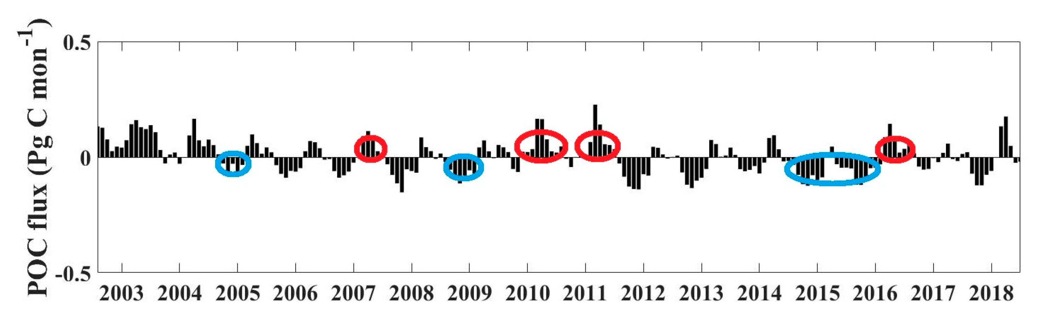
4.2. Anomalies During the Annual Decreasing of POC Flux

In Section 3.3.2, we noticed some abnormal phenomena in the downward trend of POC flux over years. In order to investigate these outliers, we depicted the relationship between monthly POC flux and month average POC flux between 2003 and 2018 (Figure 7). In Figure 7, the downward trend is very obvious. Before 2008, most of monthly POC flux is above the average, but after 2008, most POC flux is below the average. We have found several special periods in this downtrend, marked with ellipses in the POC histogram, where the red ellipse indicates an abnormal increase of POC flux, and the blue ellipse indicates an abrupt decrease. Based on the existing research and related data, we suspected this unusual phenomenon is related to the El Niño-La Niña phenomenon.

In order to verify our conjecture, we compared these phenomena with the years in which the El Niño-La Niña phenomenon occurred. Oceanic Niño Index (ONI) (3 month running mean of ERSST.v5 SST anomalies in the Niño 3.4 region (5°N–5°S, 120°–170°W)) is a good indicator of El Niño and La Niña events in the Pacific Ocean, the Climate Prediction Center has recorded ONI from 1950 to the present (https://origin.cpc.ncep.noaa.gov/). According to the statistical records, from 2003 to 2018, the El Niño phenomenon occurred in 2004–2005, 2009–2010, and 2015–2016, of which 2015–2016 is a strong El Niño and lasts for a long time, while 2007–2008, 2010–2012, and 2016–2017 is the La Niña event, of which 2010–2012 is strongest. The occurrence of the El Niño and La Niña events coincides with the mutation of the POC flux displayed in Figure 7, which proves that the change of POC flux is indeed affected by the climatic event. This also indirectly confirms our conjecture.

The El Niño event may affect NPP by altering the nutrient supply in the equatorial Pacific. During El Niño, the weakening of the equatorial trade wind reduces the equatorial upwelling in the central and eastern equatorial Pacific [66]. The weakened upwelling reduces the nutrient supply of phytoplankton and consequently decreases primary production below the climatological mean [67]. As a result, the El Niño event led to a gradual decline in POC flux in the central and eastern equatorial Pacific. Iriart and González suggested that the high surface temperature anomaly during the El Niño episode of 1997–1998 led to lower phytoplankton biomass and primary production, and reduced export of POC [68,69]. In addition, according to studies by Behrenfeld, the El Niño phenomenon will enhance the stratification of water bodies in low-latitude ocean, making it difficult for nutrients to be replenished to surface seawater [70]. These will reduce carbon dioxide in the ocean and lead to a decrease in primary productivity of phytoplankton, and the decrease of NPP directly affects the decline of POC flux. Fagan also demonstrated a decrease of POC concentration during the El Niño period from 2014 to 2015 [71]. The El Niño and La Niña events generally alternate. In contrast to the El Niño event, the La Niña event leads to an increase in particulate organic matter and a decrease in sea surface temperature [72]. Especially after the end of the strong El Niño period, phytoplankton will erupt and the POC flux will also increase.

El Niño and La Niña affect not only tropical Pacific ecosystems, but changes in global marine ecosystems by influencing high and low pressure systems, winds, and precipitation. For example, La found the mean NPP decreased from 789 to 493 ${\mathrm{mg}\mathrm{C}\mathrm{m}}^{-2}{\mathrm{d}}^{-1}$ between 2010 and 2013 in the Amundsen Sea polynya, Antarctica. However, at the same time, the NPP and POC flux showed an upward trend from 2010 to 2011 (La Niña) [73]. From observations of the Ocean Station in the northeastern subarctic Pacific between 1998 and 2000, M.S. Lipsen found that POC flux decreased during 1998 (El Niño) and increased during 1999 (La Niña) [74]. The results of these studies in different oceans are consistent with ours, and also prove the impact of El Niño on global POC flux.

Although our results confirmed that POC flux was closely related to the El Niño-La Niña phenomenon, it is not certain that this relationship applies to all ocean regions around the world. More detailed research is needed to demonstrate the attribution analysis of POC flux and NPP changes in regional ocean and whether they have a clear relationship with the El Niño-La Niña phenomenon. In future research, we will determine the effects of ocean currents, nutrients, and other parameters on regional ocean POC flux changes.

4.3. Increasing Trend of POC Flux in High-Latitude Ocean

According to our estimation results, the global POC flux is indeed decreasing year by year. The analysis of long time POC flux verifies Stramska’s conjecture about the weakening of BCP [37], which is also consistent with the prediction by most models [9,36,75]. In addition, both HOT and BATS are time series observation stations that provide in situ POC flux from 2003 to 2016. Their variation trends are good indicators of the global POC flux. Therefore, this article attempted to draw a chronological scatter plot using in situ data from these two sites. As shown in Figure 8, it can be seen from the trend lines and the equations that the POC fluxes of both sites are decreasing, which further proves that the trend analysis of the global POC flux over time based on remote sensing data observations is correct.

At present, the cause for POC flux decline has not come to an agreement. A lot of work has been done on analyzing NPP as one of the main drivers for POC flux in models [9,36,76]. For example, Marinov suggested that the reduction of nutrient supply caused by stratification in low-latitude ocean is the main driver of NPP and POC flux changes. Additionally, Laufkötter showed that the increase of grazing pressure and other loss processes caused by climate warming is an important additional factor leading to the reduction of NPP and POC flux in the future [77]. However, after running four marine ecosystem model under the RCP8.5 scenario and analyzing the results, Laufkötter showed that e-ratio changes and NPP changes are equally important for changes in POC flux [53]. It reminds us to pay attention to the impact of e-ratio when using the remote sensing data to analyze the change of POC flux, which is also the focus of subsequent research.

It can be seen from our research that the global POC flux is decreasing over time obviously, but the variation characteristic of different regions is unclear. Therefore, we divided the global ocean into three parts according to different latitudes, and performed statistical analysis on the change of POC flux in different regions. We plotted the statistical results in time series as shown in Figure 9. The POC flux of the low- and mid-latitude ocean shows a declining trend consistent with the global POC flux. It can be seen from the slope of the trend line that the POC flux in low-latitude ocean has the fastest decline rate, which is related to the wide ocean area, trade wind, ocean current, and other factors in the equatorial region. From Table 4, total POC flux of the low-latitude ocean only accounts for 28.7% of global POC flux, lower POC output and higher temperature make low-latitude ocean an important “source area” of global ocean ${\mathrm{CO}}_2$ [78]. The mid-latitude ocean is more stable and less affected by other environmental variables, so its reduction rate is lower than that in low-latitude regions. However, the total POC flux of mid-latitude ocean is higher than that of other regions, because the mid-latitude ocean has more continental shelves, and the e-ratio and NPP is becoming higher when closer to the continental shelves. The e-ratio up to 63.6% makes the POC flux as high as 61% in the mid-latitude ocean of both hemispheres, far higher than the proportion of NPP (40%), which makes the mid-latitude area an important “sink area” of global ocean ${\mathrm{CO}}_2$ [79].

Different to the mid- and low-latitude ocean, the POC flux of high-latitude ocean shows an increasing trend over time. Considering to the proportion of POC flux in high-latitude ocean of both hemispheres (8.7% and 1.5% in Table 4), the Arctic ocean is the main driver to this trend. Since NPP is an important factor affecting POC flux, we first studied the changes of NPP in the Arctic Ocean. The possible trend of NPP in Arctic Ocean over time has received a lot of attention in recent years. Arrigo and Van Dijken first reported a statistically significant increase in annual NPP of the entire Arctic Ocean, which had increased by 20% from 1998 to 2009 [80]. Arrigo extended the NPP time series to the year 2012 and demonstrated an increase of 30% [81]. Li pointed out that the Arctic’s NPP increased from 2003 to 2016, and reached a maximum of 525.74 ${\mathrm{mg}\mathrm{m}}^{-2}{\mathrm{d}}^{-1}$ in 2016 [82]. Moreover, they found a strong correlation between the increasing trend of open water area and the growing NPP in Arctic Ocean [80,82].

With the decline of global NPP, the NPP in the Arctic Ocean has shown an upward trend, which has also led to an increase in POC flux. We suspect that this is related to global warming. Global warming and polar ice melting are generally recognized, researchers noted that the extent of Arctic sea ice has rapidly declined in recent years [83,84]. The IPCC Special Report on the Ocean and Cryosphere in a Changing Climate (SROCC: https://www.ipcc.ch/srocc/home/) indicated that the global ocean has warmed unabated since 1970 and the rate of ocean warming has more than doubled since 1993. Over the last decades, global warming has led to widespread shrinking of the cryosphere, and the rates of ice loss from the Greenland and Antarctic ice sheets are increasing (SROCC). NASA (https://www.nasa.gov/) also announced that Arctic sea ice reached its annual minimum on 18 September 2019, the analysis of satellite data by NSIDC and NASA shows that the Arctic sea ice sheet shrank to 4.15 million km², surpassing 2007 and 2016 as the second lowest in satellite observation history. From 1984 to 2019, Arctic sea ice shrank rapidly at a visible rate, which has not slowed down at present. As Arctic sea ice melt, the ocean area in the high-latitude has increased year by year, leading to an increase of NPP and POC flux in the high-latitude ocean. Therefore, it is not surprising that there has been an increase in POC flux of high-latitude ocean.

5. Conclusions

The ocean plays an important role in regulating the carbon dioxide content in the atmosphere, and the transfer of carbon from the surface water to the deep ocean directly affects the ${\mathrm{CO}}_2$ flux between the ocean and the atmosphere. Therefore, the monitoring of the global ocean POC flux is of great significance for the study of global carbon cycle. Based on the in situ POC flux data, this paper compared the existing classical models of estimating POC flux using remote sensing satellite data. Then, the optimal e-ratio model and the most appropriate NPP products were selected to calculate the global ocean POC flux from 2003 to 2018. The total POC flux is between 8.5 to 14.3 Gt C per year, which is consistent with these model results from other researchers. Based on the analysis of temporal and spatial variations of POC flux, three conclusions are drawn in this paper:

Firstly, in terms of spatial distribution, the Continental Margins with water depth less than 2000 m account for less than 1/7 of the global ocean area, but the POC flux accounts for about 30% of the global POC flux. Therefore, we should combine remote sensing observations, biochemical models, and some effective methods to strengthen the monitoring and evaluation of POC flux in Continental Margins.

Secondly, POC flux decreases from 2003 to 2018, which is consistent with NPP, but there are also some abnormal increases and decreases. This paper found that the occurrence of this mutation is very consistent with the appearance of the El Niño-La Niña phenomenon. Some scholars have analyzed the effect of a single El Niño-La Niña phenomenon on POC flux and confirmed this relationship. Our results further prove that the El Niño-La Niña phenomenon has an important impact on global POC flux over a long period of time.

Thirdly, the melting of polar sea ice caused by global warming enlarges the area of ocean in the high-latitudes, which makes POC flux in high-latitude ocean increase from 2003 to 2018.

In summary, the reduction of POC flux in the ocean will inevitably lead to an increase of ${\mathrm{CO}}_2$ in the atmosphere, thereby aggravating the greenhouse effect. This paper suggests that measures to deal with greenhouse gases can include two aspects: one is to reduce anthropogenic greenhouse gas emissions, and the other is to protect the marine and terrestrial ecosystems and restore their ability to fix carbon, nitrogen, and other elements. Remote sensing technology can provide effective technical support for these measures, and we will conduct more in-depth research in subsequent studies.

References

1. Siegenthaler, U.; Sarmiento, J.L. Atmospheric carbon dioxide and the ocean. Nature 1993, 365, 119–125. [Google Scholar] [CrossRef]
2. Allison, D.B.; Stramski, D.; Mitchell, B.G. Seasonal and interannual variability of particulate organic carbon within the Southern Ocean from satellite ocean color observations. J. Geophys. Res. 2010, 115. [Google Scholar] [CrossRef] [Green Version]
3. Gómez-Robles, A. Hidden trends in the ocean carbon sink. Nature 2016, 530, 426–427. [Google Scholar]
4. Falkowski, P.G.; Barber, R.T.; Smetacek, V. Biogeochemical controls and feedbacks on ocean primary production. Science 1998, 281, 200–206. [Google Scholar] [CrossRef] [PubMed] [Green Version]
5. Sabine, C.L.; Feely, R.A.; Gruber, N.; Key, R.M.; Lee, K.; Bullister, J.L.; Wanninkhof, R.; Wong, C.; Wallace, D.W.; Tilbrook, B. The oceanic sink for anthropogenic CO2. Science 2004, 305, 367–371. [Google Scholar] [CrossRef] [PubMed] [Green Version]
6. Turner, J.T. Zooplankton fecal pellets, marine snow, phytodetritus and the ocean’s biological pump. Prog. Oceanogr. 2015, 130, 205–248. [Google Scholar] [CrossRef]
7. Manizza, M.; Buitenhuis, E.T.; Le Quéré, C. Sensitivity of global ocean biogeochemical dynamics to ecosystem structure in a future climate. Geophys. Res. Lett. 2010, 37. [Google Scholar] [CrossRef] [Green Version]
8. Lima, I.D.; Lam, P.J.; Doney, S.C. Dynamics of particulate organic carbon flux in a global ocean model. Biogeosciences 2014, 11, 1177–1198. [Google Scholar] [CrossRef] [Green Version]
9. Steinacher, M.; Joos, F.; Frölicher, T.; Bopp, L.; Cadule, P.; Cocco, V.; Doney, S.C.; Gehlen, M.; Lindsay, K.; Moore, J.K. Projected 21st century decrease in marine productivity: A multi-model analysis. Biogeosciences 2010, 7, 979–1005. [Google Scholar] [CrossRef] [Green Version]
10. Henson, S.A.; Sanders, R.; Madsen, E.; Morris, P.J.; Le Moigne, F.; Quartly, G.D. A reduced estimate of the strength of the ocean’s biological carbon pump. Geophys. Res. Lett. 2011, 38. [Google Scholar] [CrossRef] [Green Version]
11. Ducklow, H.W.; Steinberg, D.K.; Buesseler, K.O. Upper ocean carbon export and the biological pump. Oceanogr. Wash. DC Oceanogr. Soc. 2001, 14, 50–58. [Google Scholar] [CrossRef]
12. Chisholm, S.W. Oceanography: Stirring times in the Southern Ocean. Nature 2000, 407, 685. [Google Scholar] [CrossRef] [PubMed]
13. Gardner, W. Sediment Trap Sampling in Surface Waters; Cambridge University Press: Cambridge, UK, 2000. [Google Scholar]
14. Loeff, D.; Van, M.R.; Pinghe, H.; Stimac, I.; Bracher, A.; Middag, R. 234Th in surface waters: Distribution of particle export flux across the Antarctic Circumpolar Current and in the Weddell Sea during the GEOTRACES expedition ZERO and DRAKE. Deep Sea Res. Part II Top. Stud. Oceanogr. 2011, 58, 2749–2766. [Google Scholar] [CrossRef]
15. Anand, S.S.; Rengarajan, R.; Shenoy, D.; Gauns, M.; Naqvi, S. POC export fluxes in the Arabian Sea and the Bay of Bengal: A simultaneous 234Th/238U and 210Po/210Pb study. Mar. Chem. 2018, 198, 70–87. [Google Scholar] [CrossRef]
16. Choi, M.S. Estimation of POC Export Fluxes Using 234Th/238U Disequilibrium in the Amundsen Sea, Antarctic V; Chungnam National University: Daejeon, Korea, 2017. [Google Scholar]
17. Kim, H.J.; Kim, J.; Kim, D.; Chandler, M.T.; Son, S.K. Sinking Particle Flux in the Subtropical Oligotrophic Northwestern Pacific from a Short-term Sediment. Trap Experiment. Ocean Sci. J. 2018, 53, 395–403. [Google Scholar] [CrossRef]
18. Subha Anand, S.; Rengarajan, R.; Sarma, V.V.S.S. 234Th-Based Carbon Export Flux Along the Indian GEOTRACES GI02 Section in the Arabian Sea and the Indian Ocean. Glob. Biogeochem. Cycles 2018, 32, 417–436. [Google Scholar] [CrossRef]
19. Torres-Valdés, S.; Painter, S.C.; Martin, A.P.; Sanders, R.; Felden, J. Fluxes of sedimenting material from sediment traps in the Atlantic Ocean. Earth Syst. Sci. Data Discuss. 2013, 6, 541–595. [Google Scholar] [CrossRef]
20. Fan, H.; Wang, X.; Zhang, H.; Yu, Z. Spatial and temporal variations of particulate organic carbon in the Yellow-Bohai Sea over 2002–2016. Sci. Rep. 2018, 8, 7971. [Google Scholar] [CrossRef]
21. Gloege, L.; Mckinley, G.A.; Mouw, C.B.; Ciochetto, A.B. Global Evaluation of Particulate Organic Carbon Flux Parameterizations and Implications for Atmospheric pCO2: Evaluating POC Flux Parameterizations. Glob. Biogeochem. Cycles 2017, 31, 1192–1215. [Google Scholar] [CrossRef] [Green Version]
22. Buesseler, K.O.; Boyd, P.W. Shedding light on processes that control particle export and flux attenuation in the twilight zone of the open ocean. Limnol. Oceanogr. 2009, 54, 1210–1232. [Google Scholar] [CrossRef] [Green Version]
23. Eppley, R.W.; Peterson, B.J. Particulate organic matter flux and planktonic new production in the deep ocean. Nature 1979, 282, 677–680. [Google Scholar] [CrossRef]
24. Baines, S.B.; Karl, P.D.M. Why Does the Relationship Between Sinking Flux and Planktonic Primary Production Differ. Between Lakes and Oceans? Limnol. Oceanogr. 1994, 39, 213–226. [Google Scholar] [CrossRef]
25. Dunne, J.P.; Armstrong, R.A.; Gnanadesikan, A.; Sarmiento, J.L. Empirical and mechanistic models for the particle export ratio. Glob. Biogeochem. Cycles 2005, 19. [Google Scholar] [CrossRef]
26. Laws, E.A.; Falkowski, P.G.; Smith, W.O.; Ducklow, H.; McCarthy, J.J. Temperature effects on export production in the open ocean. Glob. Biogeochem. Cycles 2000, 14, 1231–1246. [Google Scholar] [CrossRef] [Green Version]
27. Laws, E.A.; D’Sa, E.; Naik, P. Simple equations to estimate ratios of new or export production to total production from satellite-derived estimates of sea surface temperature and primary production. Limnol. Oceanogr. Methods 2011, 9, 593–601. [Google Scholar] [CrossRef]
28. Dunne, J.P.; Sarmiento, J.L.; Gnanadesikan, A. A synthesis of global particle export from the surface ocean and cycling through the ocean interior and on the seafloor. Glob. Biogeochem. Cycles 2007, 21. [Google Scholar] [CrossRef] [Green Version]
29. Lutz, M.J.; Caldeira, K.; Dunbar, R.B.; Behrenfeld, M.J.; Lutz, C. Seasonal rhythms of net primary production and particulate organic carbon flux to depth describe the efficiency of biological pump in the global ocean. J. Geophys. Res. Ocean 2007, 112. [Google Scholar] [CrossRef]
30. Świrgoń, M.; Stramska, M. Comparison of in situ and satellite ocean color determinations of particulate organic carbon concentration in the global ocean. Oceanologia 2015, 57, 25–31. [Google Scholar] [CrossRef] [Green Version]
31. Yu, J.; Wang, X.; Fan, H.; Zhang, R.-H. impacts of physical and Biological processes on Spatial and temporal Variability of particulate organic Carbon in the North. Pacific Ocean. during 2003–2017. Sci. Rep. 2019, 9, 1–15. [Google Scholar] [CrossRef]
32. Stramska, M.; Bialogrodzka, J. Satellite observations of seasonal and regional variability of particulate organic carbon concentration in the Barents Sea. Oceanologia 2016, 58, 249–263. [Google Scholar] [CrossRef] [Green Version]
33. Rixen, T.; Gaye, B.; Emeis, K.-C.; Ramaswamy, V. The ballast effect of lithogenic matter and its influences on the carbon fluxes in the Indian Ocean. Biogeosciences 2019, 16, 485–503. [Google Scholar] [CrossRef] [Green Version]
34. Bopp, L.; Monfray, P.; Aumont, O.; Dufresne, J.L.; Le Treut, H.; Madec, G.; Terray, L.; Orr, J.C. Potential impact of climate change on marine export production. Glob. Biogeochem. Cycles 2001, 15, 81–99. [Google Scholar] [CrossRef] [Green Version]
35. Bopp, L.; Aumont, O.; Cadule, P.; Alvain, S.; Gehlen, M. Response of diatoms distribution to global warming and potential implications: A global model study. Geophys. Res. Lett. 2005, 32. [Google Scholar] [CrossRef]
36. Marinov, I.; Doney, S.C.; Lima, I.D.; Lindsay, K.; Moore, J.K.; Mahowald, N. North.-South. asymmetry in the modeled phytoplankton community response to climate change over the 21st century. Glob. Biogeochem. Cycles 2013, 27, 1274–1290. [Google Scholar] [CrossRef] [Green Version]
37. Stramska, M.; Cieszyńska, A. Ocean. colour estimates of particulate organic carbon reservoirs in the global ocean–revisited. Int. J. Remote Sens. 2015, 36, 3675–3700. [Google Scholar] [CrossRef]
38. Behrenfeld, M.J.; Falkowski, P.G. A consumer′s guide to phytoplankton primary productivity models. Limnol. Oceanogr. 1997, 42, 1479–1491. [Google Scholar] [CrossRef] [Green Version]
39. Behrenfeld, M.J.; Boss, E.; Siegel, D.A.; Shea, D.M. Carbon-based ocean productivity and phytoplankton physiology from space. Glob. Biogeochem. Cycles 2005, 19. [Google Scholar] [CrossRef]
40. Tao, Z.; Yan, W.; Sheng, M.; Lv, T.; Xiang, Z. A Phytoplankton Class-Specific Marine Primary Productivity Model Using MODIS Data. IEEE J. Sel. Top. Appl. Earth Obs. Remote Sens. 2017, 10, 5519–5528. [Google Scholar] [CrossRef]
41. Hung, C.C.; Tseng, C.W.; Gong, G.C.; Chen, K.S.; Chen, M.H.; Hsu, S.C. Fluxes of particulate organic carbon in the East China Sea in summer. Biogeosciences 2013, 10, 6469–6484. [Google Scholar] [CrossRef] [Green Version]
42. Hung, C.-C.; Chen, Y.-F.; Hsu, S.-C.; Wang, K.; Chen, J.F.; Burdige, D.J. Using rare earth elements to constrain particulate organic carbon flux in the East China Sea. Sci. Rep. 2016, 6, 33880. [Google Scholar] [CrossRef]
43. Sallon, A.; Michel, C.; Gosselin, M. Summertime primary production and carbon export in the southeastern Beaufort Sea during the low ice year of 2008. Polar Biol. 2011, 34, 1989–2005. [Google Scholar] [CrossRef] [Green Version]
44. Martin, J.H.; Knauer, G.A.; Karl, D.M.; Broenkow, W.W. VERTEX: Carbon cycling in the northeast Pacific. Deep Sea Res. Part A Oceanogr. Res. Pap. 1987, 34, 267–285. [Google Scholar] [CrossRef]
45. Armstrong, R.A.; Lee, C.; Honjo, J.I.; Honjo, S.; Wakeham, S.G. A new, mechanistic model for organic carbon fluxes in the ocean based on the quantitative association of POC with ballast minerals. Deep Sea Res. Part II 2002, 49, 219–236. [Google Scholar] [CrossRef]
46. Stramska, M. Particulate organic carbon in the global ocean derived from SeaWiFS ocean color. Deep Sea Res. Part I Oceanogr. Res. Pap. 2009, 56, 1459–1470. [Google Scholar] [CrossRef]
47. Duforêt-Gaurier, L.; Loisel, H.; Dessailly, D.; Nordkvist, K.; Alvain, S. Estimates of particulate organic carbon over the euphotic depth from in situ measurements. Application to satellite data over the global ocean. Deep Sea Res. Part I Oceanogr. Res. Pap. 2010, 57, 351–367. [Google Scholar] [CrossRef]
48. Pan, D.; Liu, Q.; Bai, Y. Review and suggestions for estimating particulate organic carbon and dissolved organic carbon inventories in the ocean using remote sensing data. Acta Oceanol. Sin. 2014, 33, 1–10. [Google Scholar] [CrossRef]
49. Balch, W.M.; Bowler, B.C.; Drapeau, D.T.; Lubelczyk, L.C.; Lyczkowski, E. Vertical Distributions of Coccolithophores, PIC, POC, Biogenic Silica, and Chlorophyll a Throughout the Global Ocean. Glob. Biogeochem. Cycles 2018, 32, 2–17. [Google Scholar] [CrossRef] [Green Version]
50. Friedrichs, M.; Carr, M.; Barber, R.; Scardi, M.; Antoine, D.; Armstrong, R.; Asanuma, I.; Behrenfeld, M.; Buitenhuis, E.; Chai, F. Assessing the uncertainties of model estimates of primary productivity in the tropical Pacific Ocean. J. Mar. Syst. 2009, 76, 113–133. [Google Scholar] [CrossRef] [Green Version]
51. Dugdale, R.C.; Goering, J.J. Uptake of New and Regenerated Forms of Nitrogen in Primary Productivity. Limnol. Oceanogr. 1967, 12, 196–206. [Google Scholar] [CrossRef] [Green Version]
52. Henson, S.A.; Yool, A.; Sanders, R. Variability in efficiency of particulate organic carbon export: A model study. Glob. Biogeochem. Cycles 2015, 29, 33–45. [Google Scholar] [CrossRef] [Green Version]
53. Laufkötter, C.; Vogt, M.; Gruber, N.; Aumont, O.; Bopp, L.; Doney, S.C.; Dunne, J.P.; Hauck, J.; John, J.G.; Lima, I.D. Projected decreases in future marine export production: The role of the carbon flux through the upper ocean ecosystem. Biogeosciences 2016, 13, 4023–4047. [Google Scholar] [CrossRef] [Green Version]
54. Liu, K.; Iseki, K.; Chao, S. Continental margin carbon fluxes. In The Changing Ocean Carbon Cycle: A Midterm Synthesis of the Joint Global Ocean Flux Study; Hanson, R.B., Ducklow, H.W., Field, J.G., Eds.; Cambridge University Press: Cambridge, UK, 2000; pp. 187–239. [Google Scholar]
55. Muller-Karger, F.E.; Varela, R.; Thunell, R.; Luerssen, R.; Hu, C.; Walsh, J.J. The importance of continental margins in the global carbon cycle. Geophys. Res. Lett. 2005, 32. [Google Scholar] [CrossRef] [Green Version]
56. Liu, K.-K.; Atkinson, L.; Chen, C.T.A.; Gao, S.; Hall, J.; MacDonald, R.W.; McManus, L.T.; Quiñones, R. Exploring continental margin carbon fluxes on a global scale. Eos Trans. Am. Geophys. Union 2000, 81, 641–644. [Google Scholar] [CrossRef]
57. Boyd, P.W.; Trull, T.W. Understanding the export of biogenic particles in oceanic waters: Is there consensus? Prog. Oceanogr. 2007, 72, 276–312. [Google Scholar] [CrossRef]
58. De Haas, H.; Van Weering, T.C.E.; De Stigter, H. Organic carbon in shelf seas: Sinks or sources, processes and products. Cont. Shelf Res. 2002, 22, 691–717. [Google Scholar] [CrossRef]
59. Liu, D.; Bai, Y.; He, X.; Tao, B.; Pan, D.; Chen, C.-T.A.; Zhang, L.; Xu, Y.; Gong, C. Satellite estimation of particulate organic carbon flux from Changjiang River to the estuary. Remote Sens. Environ. 2019, 223, 307–319. [Google Scholar] [CrossRef]
60. Le, C.; Lehrter, J.C.; Hu, C.; MacIntyre, H.; Beck, M.W. Satellite observation of particulate organic carbon dynamics on the Louisiana continental shelf. J. Geophys. Res. Ocean. 2017, 122, 555–569. [Google Scholar] [CrossRef]
61. Son, Y.B.; Gardner, W.D.; Mishonov, A.V.; Richardson, M.J. Multispectral remote-sensing algorithms for particulate organic carbon (POC): The Gulf of Mexico. Remote Sens. Environ. 2009, 113, 50–61. [Google Scholar] [CrossRef] [Green Version]
62. Liu, D.; Pan, D.; Yan, B.; He, X.; Wang, D.; Wei, J.-A.; Zhang, L. Remote Sensing Observation of Particulate Organic Carbon in the Pearl River Estuary. Remote Sens. 2015, 7, 8683–8704. [Google Scholar] [CrossRef] [Green Version]
63. Anand, S.S.; Rengarajan, R.; Sarma, V.; Sudheer, A.; Bhushan, R.; Singh, S. Spatial variability of upper ocean POC export in the Bay of Bengal and the Indian Ocean determined using particle-reactive 234Th. J Geophys. Res. Ocean. 2017, 122, 3753–3770. [Google Scholar] [CrossRef]
64. Wakelin, S.; Holt, J.; Blackford, J.; Allen, J.; Butenschön, M.; Artioli, Y. Modeling the carbon fluxes of the northwest European continental shelf: Validation and budgets. J. Geophys. Res. Ocean. 2012, 117. [Google Scholar] [CrossRef] [Green Version]
65. Diesing, M.; Kröger, S.; Parker, R.; Jenkins, C.; Mason, C.; Weston, K. Predicting the standing stock of organic carbon in surface sediments of the North–West European continental shelf. Biogeochemistry 2017, 135, 183–200. [Google Scholar] [CrossRef] [Green Version]
66. McPhaden, M.J. Genesis and Evolution of the 1997–98 El Nino. Science 1999, 283, 950–954. [Google Scholar] [CrossRef] [PubMed] [Green Version]
67. Strutton, P.G.; Chavez, F.P. Primary productivity in the equatorial Pacific during the 1997–1998 El Niño. J. Geophys. Res. Ocean. 2000, 105, 26089–26101. [Google Scholar] [CrossRef]
68. Iriarte, J.L.; González, H.E. Phytoplankton size structure during and after the 1997/98 El Niño in a coastal upwelling area of the northern Humboldt Current System. Mar. Ecol. Prog. Ser. 2004, 269, 83–90. [Google Scholar] [CrossRef]
69. González, H.E.; Sobarzo, M.; Figueroa, D.; Nöthig, E.-M. Composition, biomass and potential grazing impact of the crustacean and pelagic tunicates in the northern Humboldt Current area off Chile: Differences between El Niño and non-El Niño years. Mar. Ecol. Prog. Ser. 2000, 195, 201–220. [Google Scholar] [CrossRef]
70. Behrenfeld, M.J.; O′Malley, R.T.; Siegel, D.A.; Mcclain, C.R.; Sarmiento, J.L.; Feldman, G.C.; Milligan, A.J.; Falkowski, P.G.; Letelier, R.M.; Boss, E.S. Climate-driven trends in contemporary ocean productivity. Nature 2006, 444, 752–755. [Google Scholar] [CrossRef]
71. Fagan, A.J.; Moreno, A.R.; Martiny, A.C. Role of ENSO Conditions on Particulate Organic Matter Concentrations and Elemental Ratios in the Southern California Bight. Front. Mar. Sci. 2019, 6. [Google Scholar] [CrossRef] [Green Version]
72. Kawahata, H.; Gupta, L.P. Settling particles flux in response to El Nino/Southern Oscillation (ENSO) in the equatorial Pacific. In Global Environmental Change in the Ocean and on Land; Terrapub: Tokyo, Japan, 2004; pp. 95–108. [Google Scholar]
73. La, H.S.; Park, K.; Wåhlin, A.; Arrigo, K.R.; Kim, D.S.; Yang, E.J.; Atkinson, A.; Fielding, S.; Im, J.; Kim, T.-W. Zooplankton and micronekton respond to climate fluctuations in the Amundsen Sea polynya, Antarctica. Sci. Rep. 2019, 9, 1–7. [Google Scholar] [CrossRef]
74. Lipsen, M.S.; Crawford, D.W.; Gower, J.; Harrison, P.J. Spatial and temporal variability in coccolithophore abundance and production of PIC and POC in the NE subarctic Pacific during El Niño (1998), La Niña (1999) and 2000. Prog. Oceanogr. 2007, 75, 304–325. [Google Scholar] [CrossRef]
75. Taucher, J.; Oschlies, A. Can we predict the direction of marine primary production change under global warming? Geophys. Res. Lett. 2011, 38. [Google Scholar] [CrossRef] [Green Version]
76. Dutkiewicz, S.; Scott, J.R.; Follows, M. Winners and losers: Ecological and biogeochemical changes in a warming ocean. Glob. Biogeochem. Cycles 2013, 27, 463–477. [Google Scholar] [CrossRef] [Green Version]
77. Laufkötter, C.; Vogt, M.; Gruber, N.; Aita-Noguchi, M.; Aumont, O.; Bopp, L.; Buitenhuis, E.; Doney, S.; Dunne, J.; Hashioka, T. Drivers and uncertainties of future global marine primary production in marine ecosystem models. Biogeosciences 2015, 12, 6955–6984. [Google Scholar] [CrossRef] [Green Version]
78. Takahashi, T.; Sutherland, S.C.; Sweeney, C.; Poisson, A.; Metzl, N.; Tilbrook, B.; Bates, N.; Wanninkhof, R.; Feely, R.A.; Sabine, C. Global sea–air CO2 flux based on climatological surface ocean p CO2, and seasonal biological and temperature effects. Deep Sea Res. Part II 2002, 49, 1601–1622. [Google Scholar] [CrossRef]
79. Takahashi, T.; Sutherland, S.C.; Wanninkhof, R.; Sweeney, C.; Feely, R.A.; Chipman, D.W.; Hales, B.; Friederich, G.; Chavez, F.; Sabine, C.; et al. Climatological mean and decadal change in surface ocean pCO2, and net sea–air CO2 flux over the global oceans. Deep Sea Res. Part II Top. Stud. Oceanogr. 2009, 56, 554–577. [Google Scholar] [CrossRef]
80. Arrigo, K.R.; Van Dijken, G.L. Secular trends in Arctic Ocean net primary production. J. Geophys. Res. Ocean. 2011, 116. [Google Scholar] [CrossRef]
81. Arrigo, K.R.; Van Dijken, G.L. Continued increases in Arctic Ocean primary production. Prog. Oceanogr. 2015, 136, 60–70. [Google Scholar] [CrossRef]
82. Li, H.; Ke, C.; Zhu, Q.; Shu, S. Spatial-temporal variations in net primary productivity in the Arctic from 2003 to 2016. Acta Oceanol. Sin. 2019, 38, 111–121. [Google Scholar] [CrossRef]
83. Stroeve, J.C.; Serreze, M.C.; Holland, M.M.; Kay, J.E.; Malanik, J.; Barrett, A.P. The Arctic’s rapidly shrinking sea ice cover: A research synthesis. Clim. Chang. 2012, 110, 1005–1027. [Google Scholar] [CrossRef] [Green Version]
84. Onarheim, I.H.; Eldevik, T.; Smedsrud, L.H.; Stroeve, J.C. Seasonal and regional manifestation of Arctic sea ice loss. J. Clim. 2018, 31, 4917–4932. [Google Scholar] [CrossRef]
Figure 1. Comparison of in situ particulate organic carbon (POC) flux with the estimated POC flux by (a) size-fractionated phytoplankton pigment absorption (aph) based Productivity Model (SAbPM), (b) Carbon based Production Model (CbPM), and (c) Vertically Generalized Production Model (VGPM).
Remotesensing 11 02941 g001
Figure 2. Global distribution map of e-ratio at the bottom of ocean euphotic layer (2003–2018 average).
Remotesensing 11 02941 g002
Figure 3. Global distribution map of annual POC flux at the bottom of ocean euphotic layer (2003–2018 average).
Remotesensing 11 02941 g003
Figure 4. Global distribution map of annual POC sedimentation at the bottom of the ocean (2003–2018 average).
Remotesensing 11 02941 g004
Figure 5. Spatial and temporal variations of monthly total NPP, POC flux, and F POC over each 1° latitude band.
Remotesensing 11 02941 g005aRemotesensing 11 02941 g005b
Figure 6. Variation curves of global monthly total NPP and POC flux from 2003 to 2018, where the green line represents NPP, the black line represents POC flux, and the two red lines are their trend lines.
Remotesensing 11 02941 g006
Figure 7. The column figure depicting the difference of monthly POC flux and its monthly mean from 2003 to 2018, the red ellipse represents an abnormally high value, and the blue represents the opposite.
Remotesensing 11 02941 g007
Figure 8. Scatter plots of in situ POC flux at HOT and BATS observation stations from 2003 to 2016, where the yellow lines are the trend lines.
Remotesensing 11 02941 g008
Figure 9. POC flux changes in low-latitude, mid-latitude, high-latitude ocean, the points represent the total annual POC flux of each part from 2003 to 2018, the trend line and its equation are marked in the figure.
Remotesensing 11 02941 g009