A Deep Learning Semantic Segmentation-Based Approach for Field-Level Sorghum Panicle Counting

Abstract

Small unmanned aerial systems (UAS) have emerged as high-throughput platforms for the collection of high-resolution image data over large crop fields to support precision agriculture and plant breeding research. At the same time, the improved efficiency in image capture is leading to massive datasets, which pose analysis challenges in providing needed phenotypic data. To complement these high-throughput platforms, there is an increasing need in crop improvement to develop robust image analysis methods to analyze large amount of image data. Analysis approaches based on deep learning models are currently the most promising and show unparalleled performance in analyzing large image datasets. This study developed and applied an image analysis approach based on a SegNet deep learning semantic segmentation model to estimate sorghum panicles counts, which are critical phenotypic data in sorghum crop improvement, from UAS images over selected sorghum experimental plots. The SegNet model was trained to semantically segment UAS images into sorghum panicles, foliage and the exposed ground using 462, 250 × 250 labeled images, which was then applied to field orthomosaic to generate a field-level semantic segmentation. Individual panicle locations were obtained after post-processing the segmentation output to remove small objects and split merged panicles. A comparison between model panicle count estimates and manually digitized panicle locations in 60 randomly selected plots showed an overall detection accuracy of 94%. A per-plot panicle count comparison also showed high agreement between estimated and reference panicle counts (Spearman correlation ρ = 0.88, mean bias = 0.65). Misclassifications of panicles during the semantic segmentation step and mosaicking errors in the field orthomosaic contributed mainly to panicle detection errors. Overall, the approach based on deep learning semantic segmentation showed good promise and with a larger labeled dataset and extensive hyper-parameter tuning, should provide even more robust and effective characterization of sorghum panicle counts.

1. Introduction

Recent years have seen unmanned aerial systems (UAS) emerge as effective means for field-relevant phenotyping activities by enabling efficient and more affordable collection of aerial crop images over entire crop growth cycles. Traditional image analysis and machine learning have played key roles in transforming these image data into targeted phenotypic information such as plant height [1,2] and plant population counts [3,4,5]. However, the massive image data being collected by UAS and other high throughput platforms pose challenges to traditional methods, whose performance tends to level off and fall short of the high accuracy required for fully automated systems [6]. Much of the loss in performance in traditional methods is attributable to the limitations of feature engineering, which is a critical step in many of them. Feature engineering, the selection of suitable features based on domain knowledge to aid analysis, is almost always data or situation specific which presents huge challenges when massive and diverse data are involved [7]. It is not feasible to come up with a comprehensive feature set if an expert must account for variability in thousands of images. This is even more complicated in agricultural environments where image quality is influenced by changes in illumination, crop growth and senescence [4,8].

The most promising image analysis methods in that respect are those based on deep learning. Deep learning is a subset of machine learning where multi-layer artificial neural networks learn from large amounts of data to accomplish a targeted application. Deep learning provides three major advantages over traditional approaches. First, it achieves consistent and high accuracies in classifying, identifying and segmenting objects of different categories from image data. Second, its performance scales with the amount of data, thus could handle massive datasets without significant drops in accuracy. Third, the ability to adapt a pre-trained model to other applications through transfer learning, significantly reduces the burden of training [6,9]. Deep learning removes the burden and limitation of feature engineering by learning features automatically, providing an opportunity for improved automation while allowing for increases in accuracy with large data [10]. Such robust performance is likely to be useful for applied breeding by reducing the down time between the time massive images are collected and the availability of needed phenotypic data.

Sorghum (Sorghum bicolor L. Moensh) is an important food and economic crop in many parts of the world [11]. In the face of global climate change and population growth, sorghum breeders continue to strive for improved crop yields to boost food security. Plant phenotyping, the characterization of a plant’s physical attributes, is of great significance to achieving this breeding goal. In sorghum breeding, sorghum panicles, the reproductive (flowering) part of a sorghum plant and main yield component, are among the critical components for which phenotypic data are sought [12]. Phenotypic data such as counts, number of seeds per panicle, sizes (panicle length and width) play key roles in various assessments including assessing genetic diversity, selection of new cultivars and estimation of potential yields [13,14,15,16,17,18,19,20]. However, the manual characterization of panicles has proved to a bottleneck to sorghum crop improvement. Thus, approaches such as deep learning that can provide an estimate of phenotypic attributes in an effective and efficient manner are needed to expedite sorghum improvement [21,22].

Previous studies have proposed various deep learning architectures for a variety of tasks including image classification, regression, object detection and semantic segmentation [6,23,24,25]. Popular among these are convolutional neural networks (CNN), which apply sequences of convolutional layers to facilitate learning of image features [26]. Like ordinary neural networks, CNNs apply learnable weights and biases to input image values to transform them into final predictions. However, CNNs have a deep architecture consisting of multiple hidden layers (more than 3) making them more robust than ordinary neural networks. CNNs also account for local connectivity by enforcing consecutive-only neuron connections and by applying shared weights and layer pooling, reduce the complexity of training process [26]. The annual ImageNet Competitions (http://www.image-net.org/), in which participants compete to classify millions of sample images from the ImageNet database, has inspired a number of deep learning architectures. Notable examples include the VGG-16 model [23], GoogleNet by Google [27] and ResNet by Microsoft Research [24] with 16, 22, and 152 layers respectively. While all these models were originally designed for image classification, they are adaptable to other applications—the SegNet model [23] adapts VGG-16 model for semantic segmentation, RCNN [28] adapt common CNN architecture for object detection. Thus, the stage is set for the application of these models to a variety of phenotyping tasks.

The utility of deep learning has already gained ground in various plant phenotyping tasks including plant disease detection and diagnosis [29], fruits and flowers classification [30], leaf counting in rosette plants [10] and maize tassel counting [31] with relatively higher accuracies than previous methods. In a number of studies, pretrained deep learning models have been adapted to applications of interest to boost performance, given many of the pretrained models have already been trained on thousands or millions of images [29,30]. Yet, other researchers designed custom deep learning architectures to extract targeted information. In Lu et al [31], a custom deep convolutional neural network model called TasselNet was developed to count maize tassels through density-based estimation under field environments. Xiong et al [32] segmented rice panicle objects from field images based on a custom model, Panicle-SEG model, which combined super-pixel clustering and a CNN to provide robust performance. A positive outcome of previous studies is growing availability of labeled datasets that other studies can leverage. However, given the still lower state of application of deep learning analyses in plant phenotyping, there still need for more specialized datasets and evaluation of deep learning approaches to other aspects of plant phenotyping.

For sorghum panicle counting, other traditional machine learning and deep learning approaches have also previously been used [33,34]. In [33] color information and three-dimensional structure information were leveraged by using a color ratio and circle fitting approach to detect sorghum panicles. Given the reliance on color ratios and the circularity of panicles in nadir images, this approach could be limited under wide spectral variability or under shape distortion due to image capture geometry. Another study [34] applied a combination of clustering using the Simple Linear Iterative Clustering (SLIC) [35] super-pixel algorithm and bag-of-words models [36] to learn relevant features for panicle classification. Panicles were then detected based on learned features by applying a logistic regression model. While high accuracy was achievable, it came at the expense of significant feature engineering. A similar approach based on learning multiple features for panicle detection is presented in [37]. To reduce the effort spent on manual labeling, Ghosal et al. [38] applied a weakly supervised deep learning framework whereby a model was trained on a small training sample but gradually updated through human feedback on object detection results. They demonstrated a significant reduction in human labeling effort without compromising final model performance.

In this study, our main goal was to develop a field-based approach for counting sorghum panicles from UAS images using deep learning semantic segmentation. Sematic segmentation is a supervised learning problem aimed at assigning each pixel of an image to one of several semantic classes [39,40]. Our general approach relied on a SegNet model to segment UAS images into sorghum panicles and other features such as foliage and exposed ground. While we could have applied an object detection approach, we choose the semantic segmentation option because of better definition of object boundaries, which provided opportunities for splitting any merged panicle instances. Object detection only provides bounding boxes of detected objects, which might involve much more post processing [31]. Our specific objectives were to: (1) develop labeled datasets to support the semantic segmentation of panicles from existing UAS image data from sorghum trials; (2) Train and evaluate the SegNet model for semantic segmentation of UAS data into the three semantic lasses; (3) develop a method for detection and localization of individual panicles within the experimental field based on the semantic segmentation results and 4) compare derived panicle count estimates with manually collected counts.

2. Materials and Methods

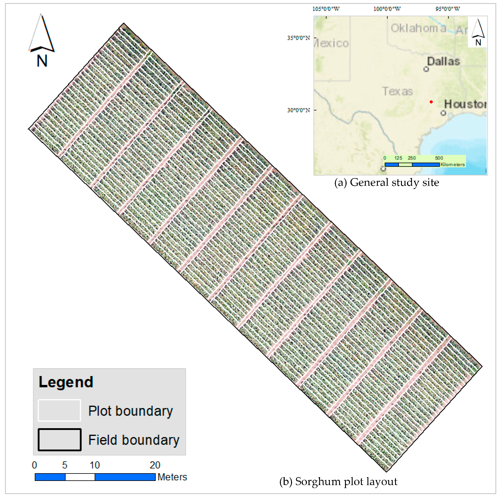
2.1. Study Site

Our study site was a sorghum experimental field on the Texas A&M AgriLife Research Farm (Latitude 30°55′00″ N, Longitude 96°25′48″ W) in Burleson County, Texas (USA). The climate in this region is humid subtropical with mild winters and hot summers [41]. The soil at the AgriLife Research Farm is a silt clay loam with 0–1% slopes [42]. The field, planted on 26 April 2017, comprised historical grain sorghum material covering over 700 single-row (0.75 m by 6.0 m) plots. For our study only 360 plots were used as shown in Figure 1. Standard agronomic practices for grain sorghum production, including supplemental irrigation and fertilization as needed, were applied.

2.2. Data

2.2.1. UAS Image Data and Plot Boundaries

We collected aerial images over the field using a DJI Phantom 3 Professional UAS (Shenzhen, Guangdong, China) with a 12-megapixel DJI FC300X camera at the following settings: a 35 mm equivalent focal length of 20, a F-stop of f/2.8 and an automatic ISO option. Images were captured on a sunny and virtually still day on 7 July 2017, when the crop was in its reproductive growth stage, from a flight altitude of 10m with 90% forward and side image overlap in a standard parallel flight pattern.

The collected images were processed using the Pix4Dmapper software to generate orthomosaics. Standard photogrammetric processing was followed including extraction and matching of common points across images followed by triangulation and bundle adjustment to generate densified 3D point clouds and orthomosaic images [1]. The effective ground sample distance of the generated orthomosaics was 0.4 cm/pixel. Ground control points were not used and image registration relied on geotagged GPS image positions only. For our purposes, only relative positions were needed, thus relying on geotagged positions was adequate. Based on the generated orthomosaics, plot boundaries were generated in shapefile format. Plot boundaries were buffered inward by a small distance (10 cm) to minimize edge effects, where panicles from one plot encroached on a neighboring plot.

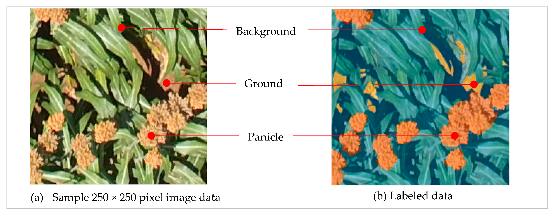
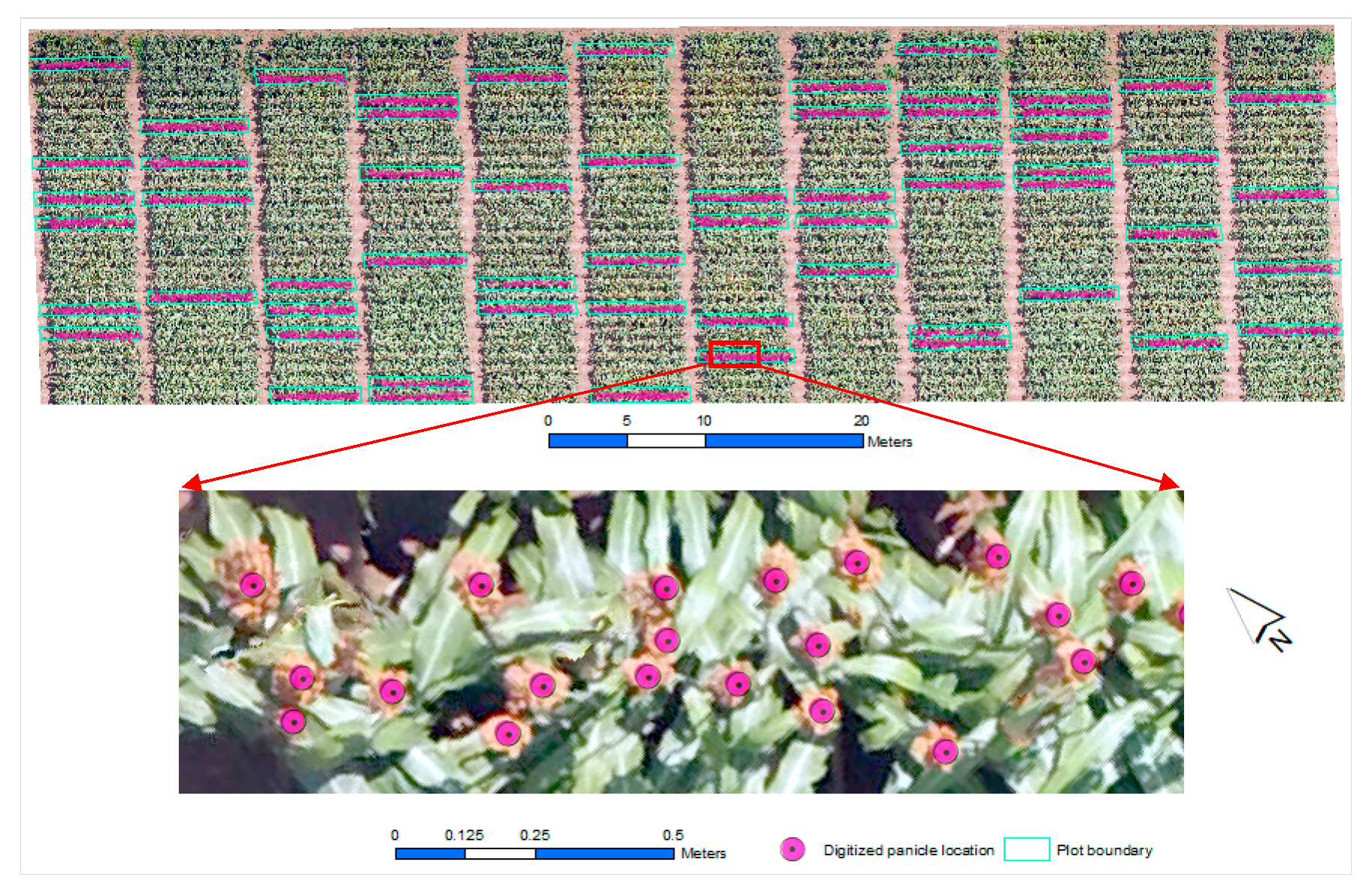
2.2.2. Labeled Panicle Data

Labeled panicle data for deep learning based semantic segmentation were developed from 250 × 250 pixels sample images cut out from full UAS scenes. Three semantic classes were defined as follows: Panicle, for all panicle instances in an image; Ground, for exposed ground surfaces in the image and; Background, for green foliage and any shadowed regions in the image as illustrated in Figure 2. The manner in which the semantic classes are modeled depends on the goal of the application. While two semantic classes (panicle and background) would have sufficed, we modeled ground as a separate class to provide a better scene characterization. In addition, ground and panicles may look similar, so modeling them separately enable a trained model to be more robust to these similarities. In selecting sample images, we tried to make the sample set as representative as possible by including various scenarios. We selected samples with panicles of different colors, samples without panicles, samples with pure classes (e.g., ground only) and samples from images captured at different angles. Labeling for semantic segmentation requires that all pixels in each sample images are labeled. Thus, we digitized all pixels in each sample into predefined semantic classes using the Image Labeler tool in the MATLAB^® software (www.mathworks.com). The Image Labeler provides an easy interface to mark a variety of regions of interest (rectangular, pixel, polygon) in sample images to define targeted ground truth for semantic segmentation and object detection. We labeled 462 samples.

2.3. Sorghum Panicle Counting Approach

Our panicle counting approach involved two main steps: (1) deep learning semantic segmentation of input image data and (2) Post-processing to facilitate individual panicle counting. The semantic segmentation served to classify and accurately locate panicles with an image. The second step post-processed the semantic segmentation output to get rid of small object sand split any merged panicles. Figure 3 summarizes our general workflow.

2.3.1. Deep Learning Semantic Segmentation and Model Fitting

Deep learning semantic segmentation overview: At a basic level, a deep learning architecture for semantic segmentation comprises an encoder and decoder network. An encoder network is normally a CNN, which learns relevant but low-resolution features about the target classes. On the other hand, a decoder network uses the learned features to generate a pixel level prediction. Previous studies in the computer sciences have developed various approaches for semantic segmentation [23,25,28,29,43,44]. Region-based and fully connected convolutional network-based (FCN) approaches are among the predominant ones. Region-based approaches such as R-CNN [28] rely on object detection—candidate regions are selectively extracted and their corresponding features computed. Then, it applies a classifier such as support vector machine for pixel level prediction to generate a semantic segmentation. While high performances are achievable using such approaches, the need to extract many candidate regions can be time-consuming. In addition, selected candidate regions may not be representative, which may lead to poor boundary definition. Like region-based methods, FCN-based methods [25] use a CNN but are able to learn and optimize pixel to pixel mappings without extracting candidate regions. However, such networks suffer from loss of resolution due to the consecutive convolutional and pooling operations. Approaches that generate high-resolution segmentations such as SegNet [44] and U-Net [43] have developed and have demonstrated improved performance.

Fitting SegNet semantic segmentation model: In this study, we adapted a SegNet with weights initialized from the VGG-16 network for semantic segmentation of sorghum panicles using MATLAB® Computer Vision and Deep Learning toolboxes. Building a SegNet type model in MATLAB only requires one to specify the size of the input sample images (250 × 250 × 3), the number of semantic classes (3) and a pretrained model, VGG-16 in our case. The rest of the network setup such as assigning weights from VGG-16 network and adding required layers is then done automatically. Given the unbalanced sampling among the three semantic classes, we incorporated sample weighting, with weights calculated as the inverse frequency of each class, to enhance the robustness of our model. To improve the accuracy of the network, we also augmented the training data by randomly shifting, rotating and reflecting it to create multiple versions of the data [45,46]. With a fully specified model, we trained it using mini-batch stochastic gradient descent with momentum (SGDM) as the optimizer with 75% of the labeled data and 15% of the data for validation. The learning rate followed a piecewise schedule that reduced the learning rate from an initial value of 0.03 by a factor of 0.3 every 10 epochs. A mini-batch size of 4 training samples was used to reduce memory usage while training. Training was accomplished over 50 epochs on a 64-bit Dell Workstation (Intel® Xeon® Processor with 256 Gb RAM, NVIDIA™ Quadro K5200 GPU with 8 Gb RAM) and took about an hour and half to complete. Having trained the model, we applied it to the field orthomosaic to generate a field-level semantic segmentation.

Accuracy assessment of trained SegNet model: We evaluated the accuracy of the trained deep learning model against remaining 10% test labeled data using two metrics: the overall accuracy (OA) and the intersection over union (IoU). The overall accuracy expresses the rate of correctly classified pixels regardless of class. The IoU segmentation measure also known as Jaccard coefficient, is the ratio of correctly classified pixels to the total number of ground truth and predicted pixels in that class—penalizes false positives. We applied these metrics to assess both global and per-class performance of the sematic segmentation. Given the number of true positives, TP, the number of true negative, TN, the number of false positives, FP and the number of false negatives, FN, we defined the two metrics as follows:

$$A=\frac{\left(TP+TN\right)}{\left(TP+TN+FP+FN\right)}\times 100$$

(1)

$$IoU=\frac{\left(TP\right)}{\left(TP+FP+FN\right)}\times 100$$

(2)

2.3.2. Post-Processing and Panicle Counting

The semantic segmentation result required post-processing before panicles we could detect individual panicles and estimate plot-level panicle counts due to: (1) existence of small usually wrong classified objects, (2) existence of merged panicle objects that affected the plot-level panicle count estimates. We applied a sequence of morphological operations and the watershed transform to alleviate these two issues.

To remove small objects, we first binarized the semantic segmentation output so 1s represented panicle regions and 0s represented everything else. We then applied an erosion operation, using a 3-pixel disk shaped structuring element, to the binarized output to remove some of the boundary pixels from all panicle objects and also get rid of some small objects. Given that we expected panicle objects to be of certain minimum size, we imposed a size (30-pixel) restriction of the eroded output by applying an area opening morphological operation. The 30-pixel threshold was determined empirically by examining sizes of panicle objects in the segmented image.

With the clean panicle mask from the preceding steps, we applied a watershed transform to split merged panicles. Watershed transform treats an image as a topographic surface with ridges and valleys and achieves a segmentation by decomposing the image into catchment basins [47,48]. To model a topographic surface from a binary image, an approach often used is to calculate a negative distance transform to the complement of a binary image (panicle mask in our case) [49]. The distance transform generates an image showing distances for each foreground pixel to the closest boundary and inverting it ensures target object center pixels are regional minima, satisfying assumptions of the watershed transform. With the watershed transform, any local minima can be catchment, which often leads to over-segmentation. To prevent over-segmentation, we suppressed some local minima in the distance transform before applying the watershed transform. We achieved this by suppressing all minima in the negative distance transform image whose depth is less than d, 0.7 in our case. We determined the threshold d through prior empirical test.

Having split the merged panicles, we applied connected components analysis to watershed transform output to generate individual panicle regions. Based on area attributes of the connected components, we eliminated any regions with area less than 30 pixels. Finally, we determined panicle locations using centroid coordinates of each connected component as illustrated in Figure 3. Having detected the panicle instances in the field, we determined plot-level panicle counts by aggregating all detected panicle instances within respective plot polygons.

2.3.3. Validating Detected Panicle Counts

We evaluated the performance of our panicle counting method both in terms of individual panicle detection and in terms of overall plot-level correlation by comparing estimated panicle counts with manually digitized panicle data. We randomly selected 60 plots and manually digitized panicle locations from the orthomosaic (Figure 4). In cases where multiple panicles touched, we digitized them as separate entities to test how effective the developed procedure would perform at separating them.

To evaluate panicle detection accuracy, we used several accuracy measures to capture overall under or over-detection of panicles. The three accuracy measures included the omission error (OE), which captured the rate at which our method missed sorghum panicles; the commission (misclassification) error (CE), which showed the rate at which our method wrongly classified other objects as panicles and; the overall accuracy (OA), which showed the overall detection rate of our method with respect to a known number of panicles. We calculated the three accuracy measures as shown in Equations (3):

$$OE=\frac{N_o}{N_R}\times 100; CE=\frac{N_m}{N_D}\times 100; OA=\frac{N_t}{N_R}\times 100$$

(3)

where N_o is the number panicle omitted, N_m is the number of wrongly classified objects, N_t is the total number of correct panicle detections, N_R is known total number of panicles and N_D is the total number of locations detected as panicle detections.

To get the total number of correctly classified panicles, N_t, we matched detected panicle locations to measured x-y panicle locations. We considered a detected panicle correctly matched if it fell in a 5 cm buffer zone around a reference panicle, selecting the 5 cm radius based on average panicle width data [5]. Where multiple panicles fell in the buffer zone, we considered only the nearest panicle to the buffer center. The number of missed panicles, N_o, was defined by the number of panicles without any detected panicle in their buffer zones while, N_m, was determined as the difference between N_d and N_t.

To capture the under and over-estimation and correlation of estimate panicle counts with respect to manually digitized panicle counts, we also calculated a mean bias, bias_avg, and Spearman’s correlation, ρ, metrics. The bias_avg for the selected number of plots was calculated as in Equation (4) where R_i is the ith reference attribute measurement, E_i is the ith computed attribute measurement and N is the total number of measurements being compared. The Spearman’s correlation was calculated using Equation (5), where $\overline{E}$ and $\overline{R}$ represented mean panicle counts for the computed and reference measurements.

$$bia{s}_{avg}=\frac{1}{N}{\displaystyle \sum }_{i=1}^N(E_i-R_i)$$

(4)

$$\rho = \frac{{\sum }_{i=1}^N\left(E_i-\overline{E}\right)\left(R_i- \overline{R}\right)}{\sqrt{{\sum }_{i=1}^N{\left(E_i-\overline{E}\right)}^2{\sum }_{i=1}^N{\left(R_i- \overline{R}\right)}^2}}$$

(5)

3. Results

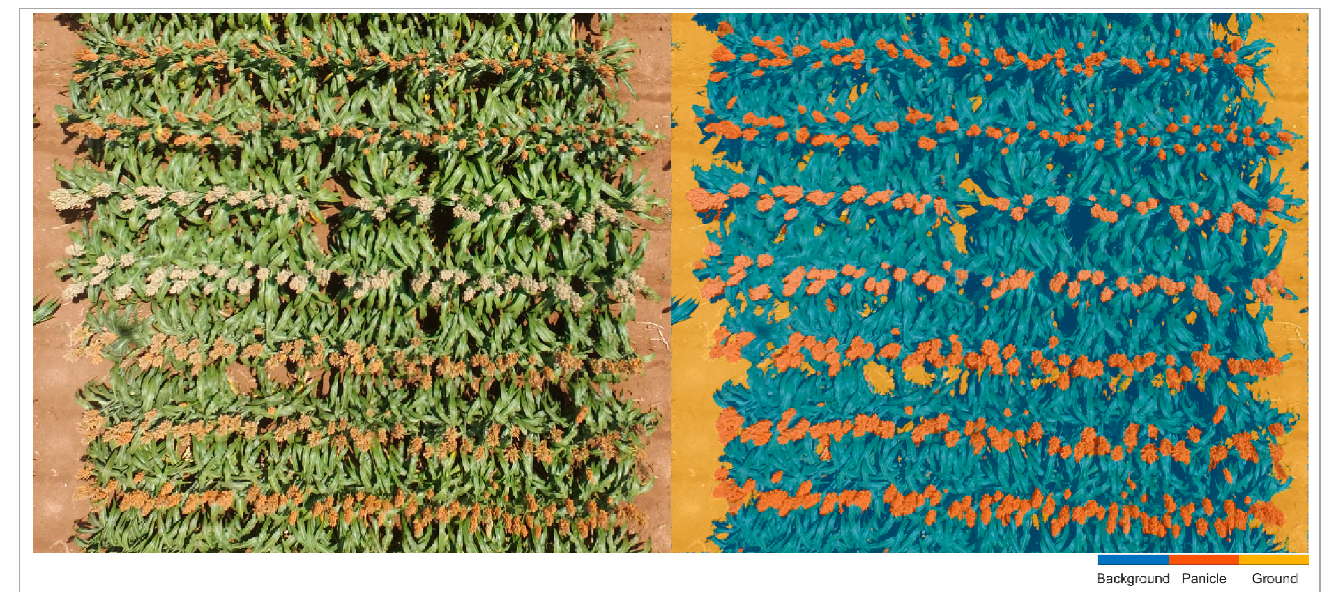
3.1. Deep Learning Semantic Segmentation

3.1.1. Overview of Results

Table 1. Performance metrics for the semantic segmentation of sorghum panicles.

Overall Performance		Per-Class Performance
Metric	Value	Class	Accuracy	IoU
Overall Accuracy	95%	Background	94%	93%
Mean IoU	87%	Panicle	95%	80%
		Ground	98%	90%

summarizes overall and class-specific accuracies for the semantic segmentation of UAS image data achieved by the trained deep learning model. The model achieved an overall accuracy of 95% with class-specific accuracies ranging from 94% to 98%. The segmentation performance in terms of intersection over union (IoU) ranged from 80–93% showing a high agreement between the deep learning segmentation and the reference labeled data. Figure 5 shows a montage of a sample input image and its corresponding segmentation output, demonstrating a generally effective segmentation of the image into the three semantic classes. The model effectively segmented panicles of different colors and generated a generally clean output with low presence of mixed pixels. One key advantage of the deep learning semantic segmentation approach to traditional object-based methods is being able to generate semantic information in a single processing step. With traditional object-based approaches, separate segmentation, classification steps and post-classification steps are usually involved [50,51].

A few aspects of our model training set up are worth emphasizing. Sample weight balancing is an important consideration for applications where semantic classes have different prevalence. Without it, less prevalent classes (panicle in our case), would not be adequately segmented. We used the inverse frequency weighting scheme, however, other weighting schemes such as over-weighting a class of interest are possible and might be of interest for further assessment [52]. While our training set was small, leveraging weights from pretrained VGG-16 model, improved the model fitting and reduced the training time. Model fitting also benefitted from data augmentation which artificially increasing the amount of data. Despite the improvements due to data augmentation, there is still a great need to develop extensive labeled datasets to enhance the generalization of fitted deep learning models.

3.1.2. Observed Sources of Error

Errors of commission among the three classes contributed to loss of performance of the semantic segmentation model. The model misclassified some dry foliage and textured ground surfaces as panicles. The segmentation was also poor around object edges as illustrated in Figure 6b. The lack of crisp edges in semantic segmentation is a well-known problem in SegNet architectures due to the down-sampling involved in the encoder part of the network [23]. Errors in segmenting panicle objects could also be attributable to the dominance of other features in scenes [53], which made it difficult for the model to segment relatively smaller panicle objects. This, together with edge errors, contributed to lowering the IoU metrics especially for panicle class (80%). Nevertheless, an IoU score of 80% was high enough to overlap all panicle instances which contributed to lower omissions of panicle objects.

While we strove to digitize each semantic class as closely as possible, we sometimes missed or sub-optimally digitized subtle objects. Small objects presented the most challenge in the labeling processes due to the difficulty in digitizing them and the image resolution limitation. However, the model was generally robust to such omissions and generated the expected output as illustrated in Figure 6c. However, such missed objects, while correctly segmented, still contributed to lowering the IoU scores because the ground truth was considered perfect. Lastly, artifacts in the orthomosaic also contributed to wrong segmentations at the field level. Errors in 3D reconstructions and orthomosaic generation are well known in UAS image processing [54,55]. Estimation based on individual images could alleviate this limitation, as was demonstrated in [56] for estimating crop cover percent.

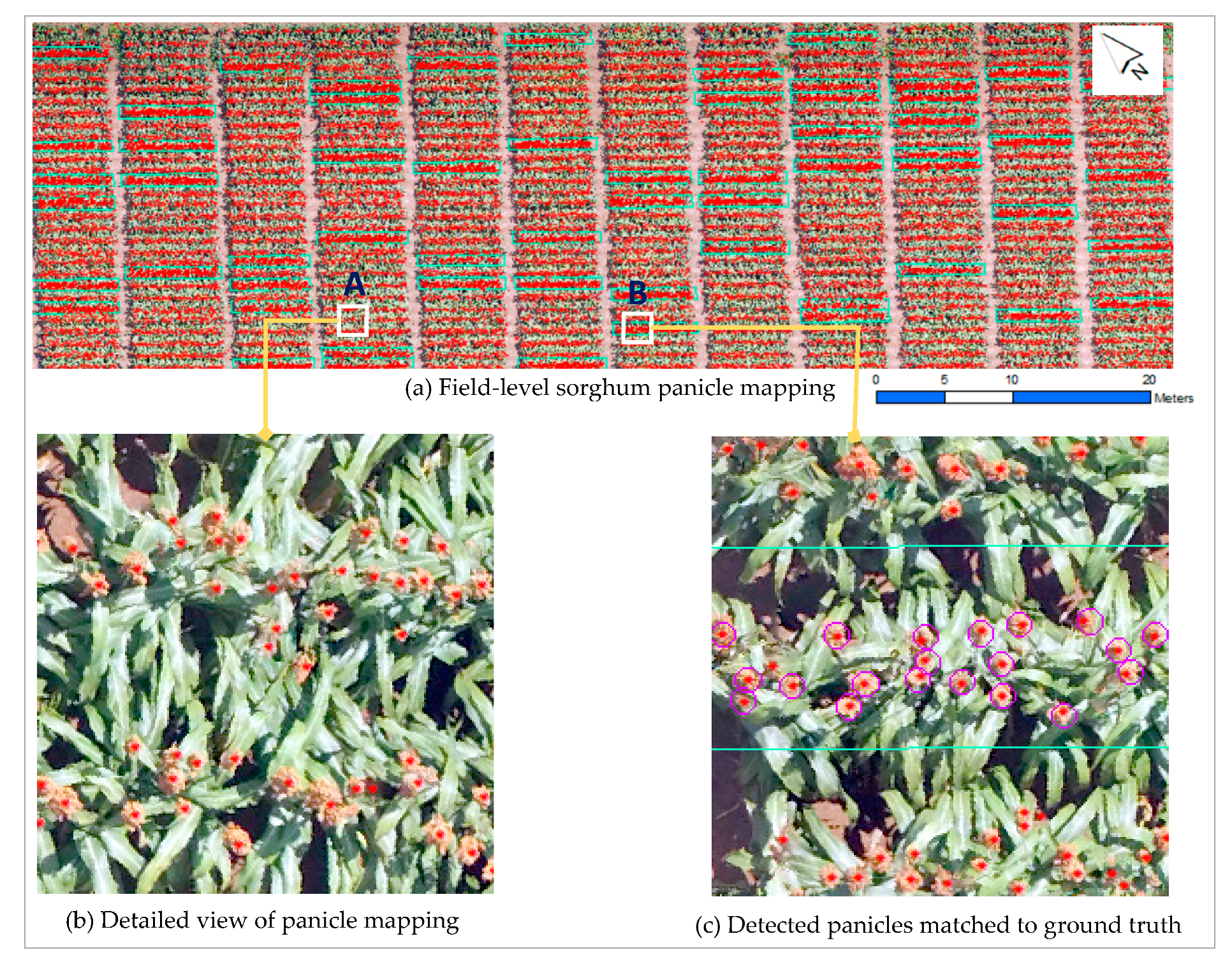
3.2. Panicle Counting Performance and Field-Level Panicle Mapping

Of the total of 3458 reference panicle locations digitized from the 60 plots, our method detected 3250, representing an overall accuracy of 94%. Our method missed 231 reference panicle locations, translating into an overall omission rate of 6.7%. We observed an overall misclassification error of 14.5% based on 3803 detections. Figure 7 shows panicles detected over the whole field with selected zoomed views to highlight a few aspects of the detection.

Differences between manual and estimated panicle counts are attributable to errors due to the deep learning semantic segmentation, as we have already outlined. However, some errors were due to the watershed segmentation. The watershed transform step erroneously split some panicle instances leading to over-counting while some merged objects were not effectively separated leading to under-counting. We observed a positive mean detection bias of 0.65 panicles, indicating a general over-estimation of panicle counts. Based on correlation, the plot-level panicle counts agreed estimates from our model with a Spearman correlation of 0.88. The over-estimation resulted mainly for the erroneous split of panicle objects. Based on the two performance metrics, the estimated panicle count compared very well with the measured panicle count in each plot (Figure 8), which shows promise for the application of deep learning approaches for such a plant phenotyping task.

The level of counting accuracy (94%) achieved in this study is an improvement from our previous study [5] (89.3%) that applied terrestrial lidar data and a density-based clustering approach. While different input data were used, we attribute the increased performance in this study to the deep learning model applied. With the development of deep learning models for point clouds [57,58], compared performance should be achieved from point clouds. Thought not directly comparable, due to the use of different accuracy metrics, the performance achieved here is generally in line to other previous studies that applied image data [34,37,38]. In Olsen et al [34] a 98% counting accuracy and median absolute error (MAE) between 1.88 and 2.66 were achieved for 18 sorghum varieties in the Midwestern United States. The accuracy was based on a receiver operating characteristic (ROC) curve’s area under the curve (AUC) metric—which is usually correlated with overall accuracy. Similarly performance was also reported in [37]. As highlighted before, this high accuracy came at the expense of significant feature engineering, which we circumvented in this study by applying a deep learning approach. Ghosal et al. [38] used 1269 hand-labeled images and achieved an AUC accuracy of 94% by applying an active learning inspired weakly supervised deep learning framework. Similar counting studies on other crops have also reported good performance. In Xiong et al [32] where rice panicles were segmented using a similar segmentation approach as ours, achieving an overall accuracy of about 83%. In counting maize tassels, [31] achieved an accuracy over 93%. The high accuracies achieved from the diverse studies is evidence of the robust performance of deep learning approaches.

4. Discussion

Plant breeding and agronomy both benefit from availability of site-specific information to manage a variety of problems [59,60]. Site-specific information within fields has traditionally been gathered by using sensors such as yield monitors or by manual sampling [21,22]. Both approaches can demand a significant amount of revenue and human resources. For example, while information on sorghum panicle number would be very useful in a breeding program, they are rarely counted because of time and labor associated with their collection. Consequently, methods developed herein offer significant improvement in site-specific panicle information for sorghum crop improvement and agronomy. These data can be leveraged by plant breeders and agronomists for site-specific data on panicle distribution, sorghum yield estimation in lieu of harvesting to obtain direct grain yield estimates. This indirect yield estimate has significant application to sorghum breeding in early phases of hybrid evaluation where relative grain yields are most important and might be estimated with combine harvest [18,61]. For agronomy, the value of indirect yield can be useful to assess yield potential prior to harvest which has numerous applications to production agriculture. For full utilization, the capacity of deep learning approach to segment panicles of different colors without additional processing is also advantageous in cases where multiple multi-color varieties are under study. While resources for developing labeled dataset may be high initially, the pay-off would be greater in ensuring years and would contribute to reducing the down time due to manual phenotyping.

With UAS image data beyond the visible spectrum now routinely being collected in many breeding programs, there is potential to enhance counting sorghum panicles with data from other non-visible wavelengths. Multispectral imagery, particularly data from the red-edge and near-infrared bands, has been applied for different aspects of plant phenotyping including in characterizing senescence patterns sorghum breading lines [62], in assessing nitrogen and chlorophyll content [63] and in assessing plant stress and disease [9,64,65]. The ability of these non-visible bands to model such subtle changes in plant condition should contribute to better discrimination of panicles from objects that are spectrally similar in the visible spectrum such as ground and dried foliage. Thermal imagery also presents another interest option, especially for characterizing canopy temperature [66,67,68]. Given the high saliency of sorghum panicles compared to other features in a field, significant temperature gradients may be expected which should be amenable to object discrimination image analysis approaches as presented in this study. Three-dimensional datasets such as digital surface models and point clouds are also promising for object detection and may enable derivation of other panicle attributes other than counts e.g., panicle lengths and widths. In our previous study [5], we demonstrated the utility of terrestrial lidar data for sorghum panicle detection and characterization of individual panicle lengths and widths. A similar study by [33] combined spectral and DSM data to estimate panicle counts and yield. With UAS-based lidar becoming more mainstream, there is a chance that such 3D data and methods will be increasingly used for panicle detection and similar applications.

While we have demonstrated the effectiveness of our developed approach, further assessments are needed to elucidate the impact of field conditions on panicle counting accuracy. Field conditions such as changes in illumination, crop growth and senescence are known to influence image quality and associated algorithm performance [4,8]. Thus, testing the effectiveness of deep learning approaches on image data collected at different times of the day or at different growth stages of a crop under study will be key in shading light on best practices and highlight challenges and limitations in the application of deep learning methods. Also, this study did not address the impact of changes in the image spatial resolution on the panicle detection. However, previous studies on UAS imaging performance have shown that lower resolution data tend to reduce the accuracy of derived metrics e.g., plant height and biomass [69,70,71]. Other studies have also shown that lower resolution images tend to lower the performance of deep learning models [72,73]. In Koziarski and Cyganek [72], the robustness of deep learning models was evaluated against distortions such as blurring and concluded that the models were susceptible to such distortions. A similar study [73] evaluated the impact of low resolution on classification accuracy of several state of art models including VGGNet [23], ResNet [24] and AlexNet [74], and also confirmed the negative impact of lower resolution on deep learning models. From the foregoing, we would recommend high resolution images, which should not only contribute to better accuracies but also allow adequate visualization of target features during ground truth labeling. Aerial imaging, as applied in this study, may also be limited in capturing significantly occluded panicles [75]. The value of applying both nadir and oblique has been demonstrated in other UAS-based studies [76,77,78]. In our case multi-angle images should provide better view of panicles and likely lead to better detection.

Research presented here could benefit from newer or alternative deep learning approaches. Notable example are instance segmentation methods, which are capable of identifying individual object instances within an image [79]. Instance segmentation usually combines an object detection step which locates the individual object instances and a semantic segmentation step that refines the object boundaries. With such capability, we could potentially eliminate the post-processing steps applied to split merged panicles. However, instance segmentation is a more challenging problem than the semantic segmentation applied here [79]. Its performance and benefits to sorghum panicle phenotyping need to be assessed in future studies. Another potential deep learning approach is density counting. Density counting enables direct counting by estimating the density of objects in the image without performing segmentation or object detection [80,81,82]. Such an approach would be useful in providing plot-level panicle counts in cases where specific location data are not needed. Previous phenotyping studies have applied this approach to count maize tassels [31] and to count plant leaves [83], which we expect can be applied for sorghum panicles too. Lastly, deep learning has, in part, been driven by the availability of large amounts of labeled datasets [6]. Continuous and extensive development of labeled datasets will be key if deep learning is to serve its intended goals in plant phenotyping. Publishing experimental data has major advantages for the research community and encourages inter-disciplinary collaborations among remote sensing scientists, plant breeders and computer scientists [84]. A few public phenotyping datasets are now available through platforms such as Cyverse, where we have published other datasets [85], but more are needed to account for the various areas of research. It is our goal to publish the labeled datasets generated for this study once all the necessary metadata has been documented.

5. Conclusions

Deep learning has revolutionized image analyses in diverse fields and the high accuracies achieved in this study show great promise for plant phenotyping tasks. By applying sample weight balancing, data augmentation and some aspects of transfer learning, we effectively trained a semantic segmentation that facilitated the estimation of sorghum panicle counts. Going by the high panicle detection accuracy, the impact of merged panicles was largely overcome by our post-processing analyses. Better accuracies can be expected with larger labeled dataset and extensive hyper-parameter tuning, for enhanced and robust field-based characterization of sorghum panicle counts. By applying such robust modeling, together with high-throughput platforms such as UAS and robots, significant gains can be expected in sorghum crop improvement and agronomy.

References

- Malambo, L.; Popescu, S.C.; Murray, S.C.; Putman, E.; Pugh, N.A.; Horne, D.W.; Richardson, G.; Sheridan, R.; Rooney, W.L.; Avant, R.; et al. Multitemporal field-based plant height estimation using 3d point clouds generated from small unmanned aerial systems high-resolution imagery. Int. J. Appl. Earth Obs. Geoinf. 2018, 64, 31–42. [Google Scholar] [CrossRef]
- Pugh, N.A.; Horne, D.W.; Murray, S.C.; Carvalho, G.; Malambo, L.; Jung, J.; Chang, A.; Maeda, M.; Popescu, S.; Chu, T.; et al. Temporal estimates of crop growth in sorghum and maize breeding enabled by unmanned aerial systems. Plant Phenome J. 2018, 1. [Google Scholar] [CrossRef]
- Gnädinger, F.; Schmidhalter, U. Digital counts of maize plants by unmanned aerial vehicles (uavs). Remote Sens. Basel 2017, 9, 544. [Google Scholar] [CrossRef]
- Shi, Y.; Thomasson, J.A.; Murray, S.C. Unmanned aerial vehicles for high-throughput phenotyping and agronomic research. PLoS ONE 2016, 11, e0159781. [Google Scholar] [CrossRef] [PubMed]
- Malambo, L.; Popescu, S.C.; Horne, D.W.; Pugh, N.A.; Rooney, W.L. Automated detection and measurement of individual sorghum panicles using density-based clustering of terrestrial lidar data. ISPRS J. Photogramm. Remote Sens. 2019, 149, 1–13. [Google Scholar] [CrossRef]
- Pound, M.P.; Atkinson, J.A.; Townsend, A.J.; Wilson, M.H.; Griffiths, M.; Jackson, A.S.; Bulat, A.; Tzimiropoulos, G.; Wells, D.M.; Murchie, E.H. Deep machine learning provides state-of-the-art performance in image-based plant phenotyping. GigaScience 2017, 6, gix083. [Google Scholar] [CrossRef]
- Najafabadi, M.M.; Villanustre, F.; Khoshgoftaar, T.M.; Seliya, N.; Wald, R.; Muharemagic, E. Deep learning applications and challenges in big data analytics. J. Big Data 2015, 2, 1. [Google Scholar] [CrossRef]
- Chopin, J.; Kumar, P.; Miklavcic, S.J. Land-based crop phenotyping by image analysis: Consistent canopy characterization from inconsistent field illumination. Plant Methods 2018, 14, 39. [Google Scholar] [CrossRef]
- Singh, A.; Ganapathysubramanian, B.; Singh, A.K.; Sarkar, S. Machine learning for high-throughput stress phenotyping in plants. Trends Plant Sci. 2016, 21, 110–124. [Google Scholar] [CrossRef]
- Ubbens, J.; Cieslak, M.; Prusinkiewicz, P.; Stavness, I. The use of plant models in deep learning: An application to leaf counting in rosette plants. Plant Methods 2018, 14, 6. [Google Scholar] [CrossRef]
- Kochsiek, A.E.; Knops, J.M. Maize cellulosic biofuels: Soil carbon loss can be a hidden cost of residue removal. GCB Bioenergy 2012, 4, 229–233. [Google Scholar] [CrossRef]
- Kumar, A.A.; Sharma, H.C.; Sharma, R.; Blummel, M.; Reddy, P.S.; Reddy, B.V.S. Phenotyping in sorghum [Sorghum bicolor (L.) moench]. In Phenotyping for Plant Breeding: Applications of Phenotyping Methods for Crop Improvement; Panguluri, S.K., Kumar, A.A., Eds.; Springer: New York, NY, USA, 2013; pp. 73–109. [Google Scholar]
- Hmon, K.P.W.; Shehzad, T.; Okuno, K. Qtls underlying inflorescence architecture in sorghum (Sorghum bicolor (L.) moench) as detected by association analysis. Genet. Resour. Crop Evol. 2014, 61, 1545–1564. [Google Scholar] [CrossRef]
- Maman, N.; Mason, S.C.; Lyon, D.J.; Dhungana, P. Yield components of pearl millet and grain sorghum across environments in the central great plains. Crop Sci. 2004, 44, 2138–2145. [Google Scholar] [CrossRef]
- Sinha, S.; Kumaravadivel, N. Understanding genetic diversity of sorghum using quantitative traits. Scientifica 2016, 2016, 3075023. [Google Scholar] [CrossRef]
- Mofokeng, A.M.; Shimelis, H.A.; Laing, M.D. Agromorphological diversity of south african sorghum genotypes assessed through quantitative and qualitative phenotypic traits. S. Afr. J. Plant Soil 2017, 34, 361–370. [Google Scholar] [CrossRef]
- Boyles, R.E.; Pfieffer, B.K.; Cooper, E.A.; Zielinski, K.J.; Myers, M.T.; Rooney, W.L.; Kresovich, S. Quantitative trait loci mapping of agronomic and yield traits in two grain sorghum biparental families. Crop Sci. 2017, 57, 2443–2456. [Google Scholar] [CrossRef]
- Rooney, W.; Smith, C.W. Techniques for developing new cultivars. In Sorghum, Origin, History, Technology and Production; Wayne, S.C., Frederiksen, R.A., Eds.; John Wiley & Sons: New York, NY, USA, 2000; pp. 329–347. [Google Scholar]
- Vogel, F. Objective Yield Techniques for Estimating Grain Sorghum Yields. Available online: https://www.nass.usda.gov/Education_and_Outreach/Reports,_Presentations_and_Conferences/Yield_Reports/Objective%20Yield%20Techniques%20for%20Estimating%20Grain%20Sorghum%20Yields.pdf (accessed on 7 December 2019).
- Ciampitti, I.A. Estimating Seed Counts in Sorghum Heads for Making Yield Projections. Available online: https://webapp.agron.ksu.edu/agr_social/eu_article.throck?article_id=344 (accessed on 5 March 2018).
- Ghanem, M.E.; Marrou, H.; Sinclair, T.R. Physiological phenotyping of plants for crop improvement. Trends Plant Sci. 2015, 20, 139–144. [Google Scholar] [CrossRef]
- Araus, J.L.; Cairns, J.E. Field high-throughput phenotyping: The new crop breeding frontier. Trends Plant Sci. 2014, 19, 52–61. [Google Scholar] [CrossRef]
- Simonyan, K.; Zisserman, A. Very deep convolutional networks for large-scale image recognition. arXiv 2014, arXiv:preprint 1409.1556. [Google Scholar]
- He, K.; Zhang, X.; Ren, S.; Sun, J. Deep residual learning for image recognition. In Proceedings of the IEEE Conference on Computer Vision and Pattern Recognition (CVPR 2016), Las Vegas, NV, USA, 27–30 June 2016; pp. 770–778. [Google Scholar]
- Long, J.; Shelhamer, E.; Darrell, T. Fully convolutional networks for semantic segmentation. In Proceedings of the IEEE Conference on Computer Vision and Pattern Recognition (CVPR 2015), Boston, MA, USA, 7–12 June 2015; pp. 3431–3440. [Google Scholar]
- Goodfellow, I.; Bengio, Y.; Courville, A. Deep Learning; MIT Press: Cambridge, MA, USA, 2016. [Google Scholar]
- Szegedy, C.; Liu, W.; Jia, Y.; Sermanet, P.; Reed, S.; Anguelov, D.; Erhan, D.; Vanhoucke, V.; Rabinovich, A. Going deeper with convolutions. In Proceedings of the IEEE Conference on Computer Vision and Pattern Recognition (CVPR 2015), Boston, MA, USA, 7–12 June 2015; pp. 1–9. [Google Scholar]
- Girshick, R.; Donahue, J.; Darrell, T.; Malik, J. Rich feature hierarchies for accurate object detection and semantic segmentation. In Proceedings of the IEEE Conference on Computer Vision and Pattern Recognition (CVPR 2014), Columbis, OH, USA, 24–27 June 2014; pp. 580–587. [Google Scholar]
- Mohanty, S.P.; Hughes, D.P.; Salathé, M. Using deep learning for image-based plant disease detection. Front. Plant Sci. 2016, 7, 1419. [Google Scholar] [CrossRef]
- Pawara, P.; Okafor, E.; Surinta, O.; Schomaker, L.; Wiering, M. Comparing Local Descriptors and Bags of Visual Words to Deep Convolutional Neural Networks for Plant Recognition. In Proceedings of the International Conference on Pattern Recognition Applications and Methods (ICPRAM 2017), Porto, Portugal, 24–26 February 2017; pp. 479–486. [Google Scholar]
- Lu, H.; Cao, Z.; Xiao, Y.; Zhuang, B.; Shen, C. Tasselnet: Counting maize tassels in the wild via local counts regression network. Plant Methods 2017, 13, 79. [Google Scholar] [CrossRef] [PubMed]
- Xiong, X.; Duan, L.; Liu, L.; Tu, H.; Yang, P.; Wu, D.; Chen, G.; Xiong, L.; Yang, W.; Liu, Q. Panicle-seg: A robust image segmentation method for rice panicles in the field based on deep learning and superpixel optimization. Plant Methods 2017, 13, 104. [Google Scholar] [CrossRef] [PubMed]
- Chang, A.; Jung, J.; Yeom, J.; Maeda, M.; Landivar, J. Sorghum panicle extraction from unmanned aerial system data. In Proceedings of the 2017 IEEE International Geoscience and Remote Sensing Symposium (IGARSS), Fort Worth, TX, USA, 23–28 July 2017; pp. 4350–4353. [Google Scholar]
- Olsen, P.A.; Ramamurthy, K.N.; Ribera, J.; Chen, Y.; Thompson, A.M.; Luss, R.; Tuinstra, M.; Abe, N. Detecting and counting panicles in sorghum images. In Proceedings of the 2018 IEEE 5th International Conference on Data Science and Advanced Analytics (DSAA), Turin, Italy, 1–3 October 2018; pp. 400–409. [Google Scholar]
- Achanta, R.; Shaji, A.; Smith, K.; Lucchi, A.; Fua, P.; Süsstrunk, S. Slic Superpixels. Available online: https://infoscience.epfl.ch/record/149300/files/SLIC_Superpixels_TR_2.pdf (accessed on 7 December 2019).
- Zhang, Y.; Jin, R.; Zhou, Z.-H. Understanding bag-of-words model: A statistical framework. Int. J. Mach. Learn. Cybern. 2010, 1, 43–52. [Google Scholar] [CrossRef]
- Guo, W.; Zheng, B.; Potgieter, A.B.; Diot, J.; Watanabe, K.; Noshita, K.; Jordan, D.R.; Wang, X.; Watson, J.; Ninomiya, S.; et al. Aerial imagery analysis–quantifying appearance and number of sorghum heads for applications in breeding and agronomy. Front. Plant Sci. 2018, 9, 1544. [Google Scholar] [CrossRef] [PubMed]
- Ghosal, S.; Zheng, B.; Chapman, S.C.; Potgieter, A.B.; Jordan, D.R.; Wang, X.; Singh, A.K.; Singh, A.; Hirafuji, M.; Ninomiya, S. A weakly supervised deep learning framework for sorghum head detection and counting. Plant Phenomics 2019, 2019, 1525874. [Google Scholar] [CrossRef]
- Chen, L.-C.; Papandreou, G.; Kokkinos, I.; Murphy, K.; Yuille, A.L. Deeplab: Semantic image segmentation with deep convolutional nets, atrous convolution, and fully connected crfs. IEEE Trans. Pattern Anal. Mach. Intell. 2018, 40, 834–848. [Google Scholar] [CrossRef]
- Erhan, D.; Szegedy, C.; Toshev, A.; Anguelov, D. Scalable object detection using deep neural networks. In Proceedings of the IEEE Conference on Computer Vision and Pattern Recognition (CVPR 2014), Columbus, OH, USA, 24–27 June 2014; pp. 2147–2154. [Google Scholar]
- Peel, M.C.; Finlayson, B.L.; McMahon, T.A. Updated world map of the köppen-geiger climate classification. Hydrol. Earth Syst. Sci. Discuss. 2007, 4, 439–473. [Google Scholar] [CrossRef]
- Hayes, C.M.; Rooney, W.L. Agronomic performance and heterosis of specialty grain sorghum hybrids with a black pericarp. Euphytica 2014, 196, 459–466. [Google Scholar] [CrossRef]
- Ronneberger, O.; Fischer, P.; Brox, T. U-net: Convolutional networks for biomedical image segmentation. In International Conference on Medical Image Computing and Computer-Assisted Intervention; Springer: Berlin, Germany, 2015; pp. 234–241. [Google Scholar]
- Badrinarayanan, V.; Kendall, A.; Cipolla, R. Segnet: A deep convolutional encoder-decoder architecture for image segmentation. IEEE Trans. Pattern Anal. Mach. Intell. 2017, 39, 2481–2495. [Google Scholar] [CrossRef]
- Shorten, C.; Khoshgoftaar, T.M. A survey on image data augmentation for deep learning. J. Big Data 2019, 6, 60. [Google Scholar] [CrossRef]
- Yu, X.; Wu, X.; Luo, C.; Ren, P. Deep learning in remote sensing scene classification: A data augmentation enhanced convolutional neural network framework. Gisci. Remote Sens. 2017, 54, 741–758. [Google Scholar] [CrossRef]
- Najman, L.; Schmitt, M. Watershed of a continuous function. Signal Process. 1994, 38, 99–112. [Google Scholar] [CrossRef]
- Hanbury, A. Mathematical morphology applied to circular data. In Advances in Imaging and Electron Physics; Hawkes, P.W., Ed.; Elsevier: Amsterdam, The Netherlands, 2003; Volume 128, pp. 124–205. [Google Scholar]
- Roerdink, J.B.; Meijster, A. The watershed transform: Definitions, algorithms and parallelization strategies. Fund. Inform. 2000, 41, 187–228. [Google Scholar] [CrossRef]
- Malambo, L. A region based approach to image classification. Appl. Geoinform. Soc. Environ. 2009, 103, 96–100. [Google Scholar]
- Blaschke, T. Object based image analysis for remote sensing. ISPRS J. Photogramm. Remote Sens. 2010, 65, 2–16. [Google Scholar] [CrossRef]
- Hand, E.M.; Castillo, C.; Chellappa, R. Doing the best we can with what we have: Multi-label balancing with selective learning for attribute prediction. In Proceedings of the Thirty-Second AAAI Conference on Artificial Intelligence, New Orleans, LA, USA, 2–7 February 2018. [Google Scholar]
- Kampffmeyer, M.; Salberg, A.-B.; Jenssen, R. Semantic segmentation of small objects and modeling of uncertainty in urban remote sensing images using deep convolutional neural networks. In Proceedings of the IEEE Conference on Computer Vision and Pattern Recognition Workshops (CVPR 2016), Las Vegas, NV, USA, 27–30 June 2016; pp. 1–9. [Google Scholar]
- Song, H.; Yang, C.; Zhang, J.; Hoffmann, W.C.; He, D.; Thomasson, J.A. Comparison of mosaicking techniques for airborne images from consumer-grade cameras. J. Appl. Remote Sens. 2016, 10, 016030. [Google Scholar] [CrossRef]
- Gross, J.W. A comparison of orthomosaic software for use with ultra high resolution imagery of a wetland environment. In Center for Geographic Information Science and Geography Department; Central Michigan University: Mount Pleasant, MI, USA, 2015; Available online: http://www. imagin. org/awards/sppc/2015/papers/john_gross_paper (accessed on 7 December 2019).
- Duan, T.; Zheng, B.; Guo, W.; Ninomiya, S.; Guo, Y.; Chapman, S.C. Comparison of ground cover estimates from experiment plots in cotton, sorghum and sugarcane based on images and ortho-mosaics captured by uav. Funct. Plant Biol. 2017, 44, 169–183. [Google Scholar] [CrossRef]
- Qi, C.R.; Su, H.; Mo, K.; Guibas, L.J. Pointnet: Deep learning on point sets for 3d classification and segmentation. In Proceedings of the IEEE Conference on Computer Vision and Pattern Recognition (CVPR 2017), Honolulu, HI, USA, 22–25 July 2017; pp. 652–660. [Google Scholar]
- Li, Y.; Bu, R.; Sun, M.; Wu, W.; Di, X.; Chen, B. Pointcnn: Convolution on x-transformed points. In Proceedings of the Advances in Neural Information Processing Systems (NIPS 2018), Montreal, QC, Canada, 4–6 December 2018; pp. 820–830. [Google Scholar]
- Robertson, M.; Isbister, B.; Maling, I.; Oliver, Y.; Wong, M.; Adams, M.; Bowden, B.; Tozer, P. Opportunities and constraints for managing within-field spatial variability in western australian grain production. Field Crop. Res. 2007, 104, 60–67. [Google Scholar] [CrossRef]
- Zhang, C.; Kovacs, J.M. The application of small unmanned aerial systems for precision agriculture: A review. Precis. Agric. 2012, 13, 693–712. [Google Scholar] [CrossRef]
- Beil, G.; Atkins, R. Estimates of general and specific combining ability in f1 hybrids for grain yield and its components in grain sorghum, sorghum vulgare pers. 1. Crop Sci. 1967, 7, 225–228. [Google Scholar] [CrossRef]
- Potgieter, A.B.; George-Jaeggli, B.; Chapman, S.C.; Laws, K.; Suárez Cadavid, L.A.; Wixted, J.; Watson, J.; Eldridge, M.; Jordan, D.R.; Hammer, G.L. Multi-spectral imaging from an unmanned aerial vehicle enables the assessment of seasonal leaf area dynamics of sorghum breeding lines. Front. Plant Sci. 2017, 8, 1532. [Google Scholar] [CrossRef] [PubMed]
- Li, J.; Shi, Y.; Veeranampalayam-Sivakumar, A.-N.; Schachtman, D.P. Elucidating sorghum biomass, nitrogen and chlorophyll contents with spectral and morphological traits derived from unmanned aircraft system. Front. Plant Sci. 2018, 9, 1406. [Google Scholar] [CrossRef] [PubMed]
- Pugh, N.A.; Han, X.; Collins, S.D.; Thomasson, J.A.; Cope, D.; Chang, A.; Jung, J.; Isakeit, T.S.; Prom, L.K.; Carvalho, G.; et al. Estimation of plant health in a sorghum field infected with anthracnose using a fixed-wing unmanned aerial system. J. Crop Improv. 2018, 32, 861–877. [Google Scholar] [CrossRef]
- Li, L.; Zhang, Q.; Huang, D. A review of imaging techniques for plant phenotyping. Sensors 2014, 14, 20078–20111. [Google Scholar] [CrossRef] [PubMed]
- Ludovisi, R.; Tauro, F.; Salvati, R.; Khoury, S.; Mugnozza Scarascia, G.; Harfouche, A. Uav-based thermal imaging for high-throughput field phenotyping of black poplar response to drought. Front. Plant Sci. 2017, 8, 1681. [Google Scholar] [CrossRef]
- Gómez-Candón, D.; Virlet, N.; Labbé, S.; Jolivot, A.; Regnard, J.-L. Field phenotyping of water stress at tree scale by uav-sensed imagery: New insights for thermal acquisition and calibration. Precis. Agric. 2016, 17, 786–800. [Google Scholar] [CrossRef]
- Chapman, S.C.; Zheng, B.; Potgieter, A.; Guo, W.; Frederic, B.; Liu, S.; Madec, S.; de Solan, B.; George-Jaeggli, B.; Hammer, G. Visible, near infrared, and thermal spectral radiance on-board uavs for high-throughput phenotyping of plant breeding trials. Biophys. Biochem. Charact. Plant Species Stud. 2018, 3, 275. [Google Scholar]
- Ni, W.; Sun, G.; Pang, Y.; Zhang, Z.; Liu, J.; Yang, A.; Wang, Y.; Zhang, D. Mapping three-dimensional structures of forest canopy using uav stereo imagery: Evaluating impacts of forward overlaps and image resolutions with lidar data as reference. IEEE J. Stars 2018, 11, 3578–3589. [Google Scholar] [CrossRef]
- Domingo, D.; Ørka, H.O.; Næsset, E.; Kachamba, D.; Gobakken, T. Effects of uav image resolution, camera type, and image overlap on accuracy of biomass predictions in a tropical woodland. Remote Sens Basel 2019, 11, 948. [Google Scholar] [CrossRef]
- Torres-Sánchez, J.; López-Granados, F.; Serrano, N.; Arquero, O.; Peña, J.M. High-throughput 3-d monitoring of agricultural-tree plantations with unmanned aerial vehicle (uav) technology. PLoS ONE 2015, 10, e0130479. [Google Scholar] [CrossRef]
- Dodge, S.; Karam, L. Understanding how image quality affects deep neural networks. In Proceedings of the 2016 Eighth International Conference on Quality of Multimedia Experience (QoMEX), Lisbon, Portugal, 6–8 June 2016; pp. 1–6. [Google Scholar]
- Koziarski, M.; Cyganek, B. Impact of low resolution on image recognition with deep neural networks: An experimental study. Int. J. Appl. Math. Comput. Sci. 2018, 28, 735. [Google Scholar] [CrossRef]
- Krizhevsky, A.; Sutskever, I.; Hinton, G.E. Imagenet classification with deep convolutional neural networks. In Proceedings of the Advances in Neural Information Processing Systems (NIPS 2012), Lake Tahoe, NV, USA, 3–8 December 2012; pp. 1097–1105. [Google Scholar]
- Bao, Y.; Tang, L. Field-based robotic phenotyping for sorghum biomass yield component traits characterization using stereo vision. IFAC Pap. 2016, 49, 265–270. [Google Scholar] [CrossRef]
- Lin, Y.; Jiang, M.; Yao, Y.; Zhang, L.; Lin, J. Use of uav oblique imaging for the detection of individual trees in residential environments. Urban For. Urban Green. 2015, 14, 404–412. [Google Scholar] [CrossRef]
- Wierzbicki, D. Multi-camera imaging system for uav photogrammetry. Sensors 2018, 18, 2433. [Google Scholar] [CrossRef]
- Nesbit, P.R.; Hugenholtz, C.H. Enhancing uav–sfm 3d model accuracy in high-relief landscapes by incorporating oblique images. Remote Sens Basel 2019, 11, 239. [Google Scholar] [CrossRef]
- Romera-Paredes, B.; Torr, P.H.S. Recurrent instance segmentation. In European Conference on Computer Vision; Springer: Berlin, Germany, 2016; pp. 312–329. [Google Scholar]
- Fiaschi, L.; Köthe, U.; Nair, R.; Hamprecht, F.A. Learning to count with regression forest and structured labels. In Proceedings of the 21st International Conference on Pattern Recognition (ICPR 2012), Tsukuba, Japan, 11–15 November 2012; pp. 2685–2688. [Google Scholar]
- Boominathan, L.; Kruthiventi, S.S.; Babu, R.V. Crowdnet: A deep convolutional network for dense crowd counting. In Proceedings of the 24th ACM International Conference on Multimedia; ACM: New York, NY, USA, 2016; pp. 640–644. [Google Scholar]
- Onoro-Rubio, D.; López-Sastre, R.J. Towards perspective-free object counting with deep learning. In European Conference on Computer Vision; Springer: Berlin, Germany, 2016; pp. 615–629. [Google Scholar]
- Dobrescu, A.; Valerio Giuffrida, M.; Tsaftaris, S.A. Leveraging multiple datasets for deep leaf counting. In Proceedings of the IEEE International Conference on Computer Vision (ICCV 2017), Venice, Italy, 22–29 October 2017; pp. 2072–2079. [Google Scholar]
- Arend, D.; Junker, A.; Scholz, U.; Schüler, D.; Wylie, J.; Lange, M. Pgp repository: A plant phenomics and genomics data publication infrastructure. Database 2016, 2016. [Google Scholar] [CrossRef]
- Murray, S.C.; Malambo, L.; Popescu, S.; Cope, D.; Anderson, S.L.; Chang, A.; Jung, J.; Cruzato, N.; Wilde, S.; Walls, R.L. G2f Maize uav Data, College Station, Texas 2017. CyVerse Data Commons: 2019. Available online: https://www.doi.org/10.25739/4ext-5e97 (accessed on 7 December 2019).