1. Introduction
Carrier-phase measurements are essential for high-precision positioning with Global Navigation Satellite System (GNSS), such as real-time kinematic (RTK) positioning and precise point positioning (PPP), since they are much more accurate than pseudoranges. Continuous tracking of the carrier-phase signals ensures that the resolved integer ambiguities remain unchanged. However, carrier-phase measurements often suffer from cycle slips because of sudden change of satellite geometry or under condition of strong atmospheric effects such as for instance ionospheric scintillation [
1,
2,
3], which results in integer ambiguity biased by an unknown integer. The corresponding carrier-phase measurement will also be biased by one to 1 million cycles. Generally, each cycle of slip can easily introduce a range error of ~20 cm to the phase measurements on frequency L1 [
4]. Such unexpected slips should be detected, and repaired if possible or addressed by introducing and estimating a new ambiguity parameter alongside the other unknowns to avoid affecting the centimeter- to millimeter-level positioning and navigation accuracy.
Many algorithms dedicated to cycle-slip detection have been developed in recent years. Most of these methods used phase combinations and phase/code range combinations in both frequencies. For example, the TurboEdit method has exploited the Hatch-Melbourne-Wübbena (HMW) linear combination together with ionospheric residual combinations in undifferenced or double-differenced dual-frequency observations [
5,
6,
7,
8]. Moreover, linear combinations with triple-frequency observations are more dedicated to extra-long wavelength, accurate time-differenced ionospheric prediction, optimized geometry-free phase combinations and minimization of the impact of code measurements [
9,
10,
11]. However, the choice of optimum combinations becomes practically difficult given diversity of equipment and these methods are not suitable for observation with only single-frequency [
12]. As a result, method suitable for single frequency or in which the individual signal of each frequency is treated as independent observation has drawn increasing interest [
4,
13,
14]. Such methods can generally be placed in two categories.
The first category includes methods based on time-series analysis of observations. Blewitt employed phase-code comparison and Doppler integration to detect cycle slips [
15]. Lichtenegger proposed a polynomial-fitting method [
16], and Kleusberg applied higher order time differences of carrier-phase observations to detect cycle slips [
17]. Each of these methods has its limitations. The code-phase comparison method is not suitable for small cycle slips due to measurement noise and multipath in the pseudorange. Moreover, having smooth phase observations is an underlying assumption of many of these methods, and this assumption is easily violated.
The second category includes methods relying on statistical quality control. These methods regard cycle slips as outliers to be separated with various mathematical models. The idea originates from Baarda and Teunissen [
18,
19,
20]. Several of these methods were developed to detect and identify cycle slip. De Lacy and Zhang exploited the Bayesian approach for undifferenced observations [
21,
22]. Song used robust estimation to deal with cycle slips that cannot be modeled [
23]. Kirkko-Jaakkola and Fujita used Receiver Autonomous Integrity Monitoring (RAIM) methodology to process the cycle slip on time-differenced observations [
24,
25]. Teunissen studied the GNSS integrity about outliers and slips on single-receiver [
26]. More recently, Zangeneh-nejad extended these methods to fix cycle slips based on the generalized likelihood ratio test [
27], and Li developed an enhanced cycle-slip detection and repair algorithm with integer least-squares estimation that is applicable to real-time single-frequency data [
28].
Cycle slips can be satisfactorily detected using most, if not all of the above methods in benign environments. The latter quality control approach is in favor because it is robust to small cycle slips even in adverse situations, and is feasible to enhance mathematical models. However, these publications have not studied in detail about the correct-detection and false-alarm rates, which is crucial in real-time data processing. For example, noisy measurements may disturb cycle-slip detection results, which will lead to low correct-detection rates and high false-alarm rates. A cycle-slip-detection method with a high correct-detection rate and a low undetection rate for single frequency observation is desired.
According to the idea of outliers’ detection and RAIM, we propose a new cycle-slip detection method aiming at high correct-detection rate and low false-alarm rate. In this method, the epoch when the cycle slips appear is determined based on a chi-square test. Then, the fuzzy-cluster algorithm is employed to identify the satellite where the cycle slip occurs. The purpose of fuzzy-cluster algorithm is generally to separate a dataset into subsets according to their similarities and dissimilarities [
29]. This useful tool is commonly used in data analysis with reasonable and satisfactory clustering results [
30,
31,
32,
33,
34].
We next describe the new proposed fuzzy-cluster-based method and its application in cycle-slip detection in detail. Afterwards, numerical experiments are conducted to assess the performance of the new method compared to the current robust estimation method using real single-frequency data with simulated cycle slips. Finally, some conclusions are drawn and the outlook for future research is discussed.
2. The New Fuzzy-Cluster-Based Method
We propose a fuzzy-cluster-based cycle-slip detection method using time-differenced single-frequency GPS carrier-phase measurements. Similar to the current robust-estimation-based cycle-slip detection method [
27], the new method consists of two steps but with different mathematical models. The first step is to identify the epoch when cycle slips appear and the second step is to determine the satellite which suffers from cycle slips. The mathematical models used and the implementation of the proposed cycle-slip detection method are demonstrated in detail in the section.
2.1. Epoch Identification of Cycle Slip
The raw observation equation of the GPS L1 measurement can be formulated as [
35]:
where the superscript
j identifies a satellite;
is the range between the receiver antenna and the phase center of the satellite, including displacements due to earth tides, ocean loading, and relativistic effects;
and
are the clock offsets of receiver
r and satellite
j, respectively;
is the slant ionospheric delay on the L1 frequency of satellite
j;
is the slant tropospheric delay;
and
are respectively the wavelength of the signal and the integer ambiguity in cycles;
and
are respectively the receiver and satellite uncalibrated hardware phase delays; and
is the carrier-phase measurement noise.
Differentiating the observations with respect to time, some parameters that remain constant, slowly varying or corrected with current models can be eliminated. The geometry-based and time-differenced observation equation is formulated as:
where
is the difference operator between two adjacent epochs, and the other symbols are defined above. It is known that the variation of the ambiguity parameter
is zero for continuous observations while an integer value when cycle slips appear. Assuming there are
n available satellites on L1 frequency signals tracked by a receiver and there is no cycle slip, all observation equations of each satellite in form of Equation (2) can be expressed as:
where
are three position parameters and one clock parameter for a moving receiver;
; and
A is the design matrix, which can be easily obtained by computing the partial derivatives of Equation (2) with respect to the estimated parameters. If there is no cycle slip, the quadratic form of the least-square residual of Equation (3) follows a Chi-squared distribution:
where
is the post residuals for all satellites resolved from Equation (3) and
is the weight matrix depending on elevation angle.
is the significance level, and
is the number of degrees of freedom for the Chi-square test. The specified
and the corresponding
can determine a threshold. When there is indeed no cycle slips,
is smaller than the threshold and the Chi-squared distribution in Equation (4) is workable. However, if
is larger than the threshold, it can be considered that the assumption that there is no cycle slip is wrong. In this case, the variation of the ambiguity parameter
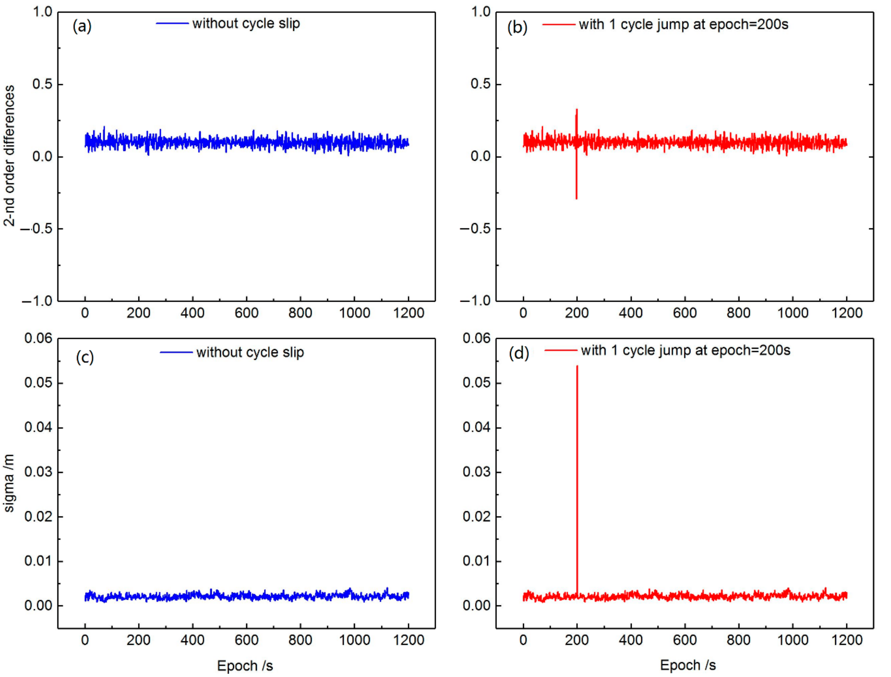
is no longer zero and there is at least one cycle slip at this epoch. This can be illustrated with
Figure 1. If there is no cycle slip, the
keeps on millimeter level. Once cycle slip occurs, the corresponding
will increase significantly. So we can determine the epoch when cycle slip occurs according to
with chi-square test.
2.2. Satellite Identification of Cycle Slip
As mentioned above, Equation (3) is formed under the assumption that there is no cycle slip. Therefore, appearance of cycle slips mean there are gross errors in Equation (3). Once gross errors appear, we can detect the outliers with some methods such as robust estimation, Bayesian estimation, RAIM, and so on. Among these methods, the RAIM method is expected to achieve a high correct detection rate [
24,
25], which is curial for real-time GPS observation quality control. Hence, we apply a fuzzy-cluster involved RAIM method to detect the satellite suffering from cycle slips in Equation (3) in this paper. Its procedure consists of decorrelation for the design matrix and then cluster for all satellites.
Firstly, the decorrelation for design matrix
A can be realized by means of Householder transformations [
36], which is a decomposition of the matrix
A into an orthogonal matrix and an upper triangular matrix as:
where
, derived from
, is an orthogonal matrix described with sub-matrix
and
in this paper.
, derived from
, is an upper triangular matrix divided into sub-matrix
and a zero matrix
. Flag
, then, according to the parity detection theory [
36], the parity detection vector composed of the matrix
T and post residuals
resolved from Equation (3) can be formed as:
where
is the parity detection vector in the parity detection theory [
36]. If there is at least one cycle slip, the
will become large because of containing the unknown integer, which is the same for
. Hence, we put the
and all satellites together and then cluster them into two subsets to separate the satellites suffering from cycle slips, which is expressed as:
we recognize that
is a sample of
n+1 observations in
m-dimensional Euclidean space.
Then, we use the fuzzy-cluster algorithm to separate the dataset
into two subsets. It should be note herein that the one of two subsets that contains
represents the satellites suffering from cycle slips. That is to say, the samples categorized with
correspond to the satellites to be identified. In the following, the fuzzy-cluster algorithm is explained in detail. Two cluster centers are marked as:
and the desired optimal cluster criterion is to minimize the objective function that is the generalized form of the least-squared error function [
32]:
where
p is the weighting fuzziness parameter, which is generally chosen as 2 [
30,
31,
32,
33,
34];
is the membership value of the
sample in the
cluster.
must satisfy the following three conditions:
In detail, the steps of this fuzzy-cluster algorithm are as follows.
Step 1. Fix the weighting fuzziness parameter and the iteration termination condition parameter .
Step 2. Given initials randomly , let the count of iterations .
Step 3. Compute cluster centers using the following equation:
Step 4. Update
with
using the following equation:
Step 5. Compute . If , then stop; else and return to Step 3.
2.3. Implementation of the New Approach
As mentioned above, each sample can obtain two membership values that belong to every cluster center in fuzzy-cluster algorithm. The sample, corresponding to one satellite, with the larger membership value belonging to cluster
is more likely to suffer from cycle slip. In the parity detection theory, after decorrelation for the design matrix, the
owned the higher correlation where
is most likely the outlier [
35]. That is to say, the larger of the membership belongs to cluster
, the most likely to be satellite suffering from cycle slip. To detect the cycle slip, we choose satellites that are most likely without cycle slips according to the membership one by one to verify with the Chi-square test. If the verification passes, we consider all of the selected satellites are without cycle slip and continue to choose a new satellites from the rest of the satellites. Until the verification fails, we think this new satellite and all the rest satellites are suffering from cycle slips. In addition, there are at least four satellites visible to achieve positioning, so we consider that the number of satellites without cycle slips is no less than four. The detailed procedure are as follows: we first select four data points that have the smallest membership value belonging to cluster
who are unlikely to suffer from cycle slip. Then the one with the smallest membership value belonging to cluster
among the rest satellites is selected and formed the observation equations together with the four satellites initially selected in form of Equation (3). Afterwards, a chi-square test is performed on the posteriori residual of the new formed equations. If the test passes, we can think that the new selected satellite does not suffer from cycle slip and the iteration can be continued. Otherwise, it will be detected as cycle slip and the iteration stops.
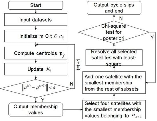
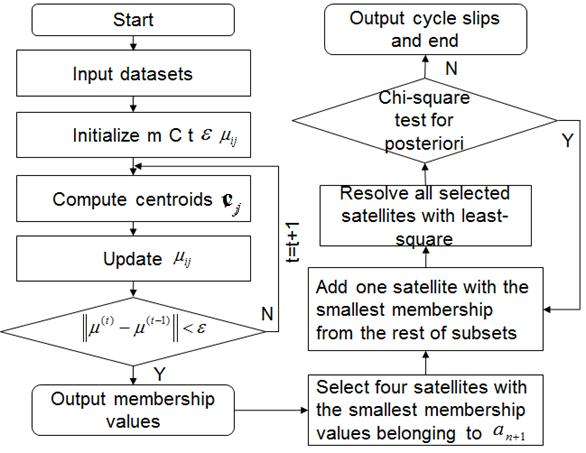
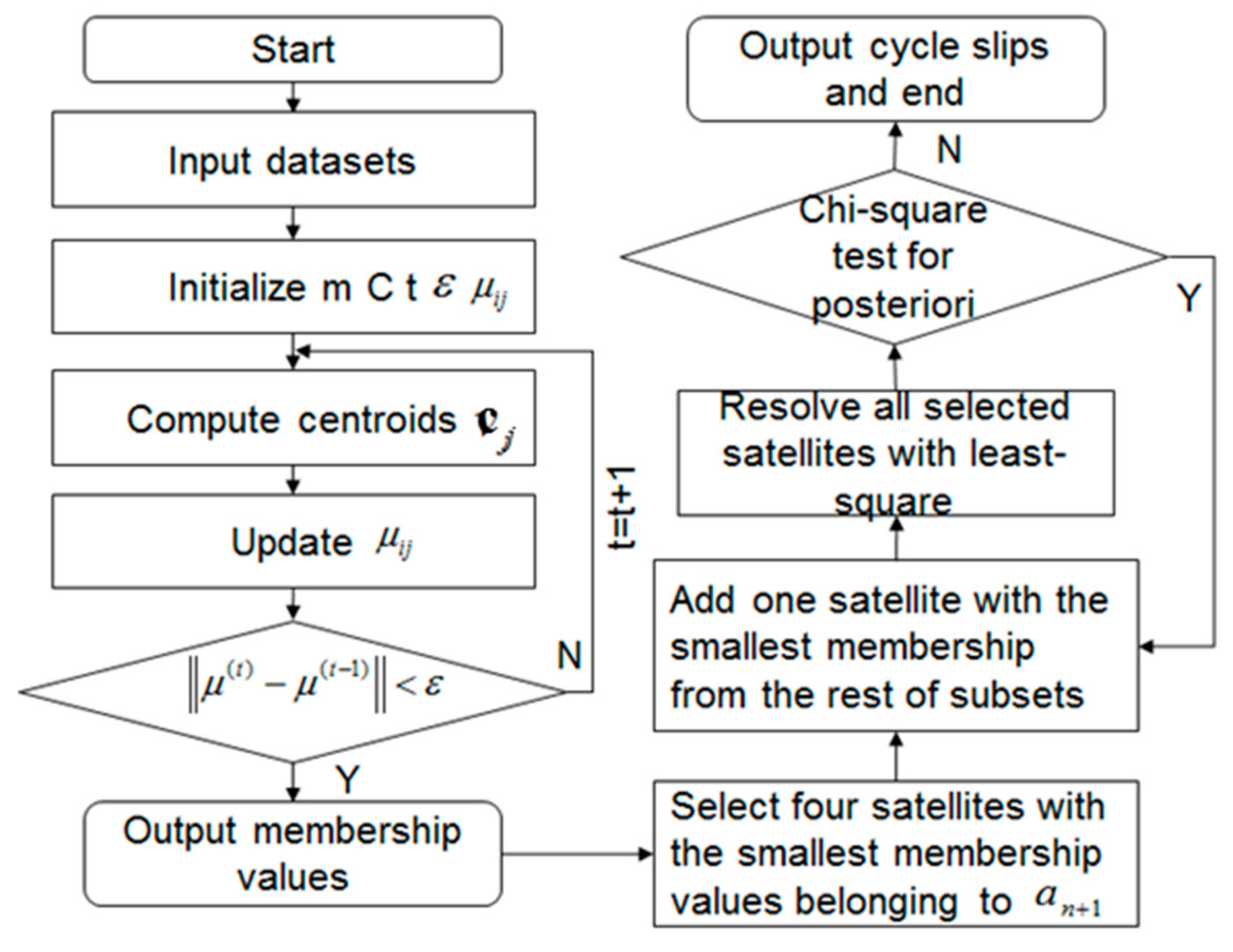
Figure 2 shows the flowchart of this procedure.
3. Experiments and Result
Considering that the proposed method is similar to the current robust estimation method, we compare the new method with the robust estimation method to validate the proposed method. Experiments are conducted as: (1) Performance of the robust estimation method (method I) and the proposed method (method II) at a single epoch with various numbers of simulated cycle slips was compared and analyzed to preliminarily investigate the effectiveness of the proposed method; (2) Performance of these two methods with various numbers of cycle slips in multiple epochs was compared; (3) Statistical results were computed. Three indicators were considered to assess the performance of the proposed method. The first one is the correct-detection rate, which is the number of correctly detected cycle slips divided by the total number of detected cycle slips. The second one is the undetection rate, which is the number of undetected cycle slips divided by the total number of simulated cycle slips. The last one is the false-detection rate, which is the number of false detected cycle slips divided by the total number of detected cycle slips. The false-detection rate means how many correct measurements were treated as a cycle slip.
3.1. Data and Experiment Description
Observations of a real GPS dataset, collected by a LEICA receiver with a LEIAR25 antenna on 21 May 2016, were used. This geodetic receiver provided phase observations on L1. We have assumed a good environment for the test, such as static receiver and free of multipath. Since it is easier to accurately simulate cycle slips after the raw observables are confirmed to be cycle-slip-free, we checked the raw data carefully and selected signals with a length of 1200 seconds from 00:21:30 to 00:41:30. Models and estimated parameters were described in detail in
Table 1. Only GPS L1 measurements were collected and all parameters were estimated single-epoch. Experiments were designed as follows. Various numbers of cycle slips with a size of one cycle on single and multiple epochs were simulated and detected using the robust estimation method and proposed method. Their performances were analyzed in detail. Moreover, the correct-detection rates and undetection rates were computed.
3.2. Performance of Single-Epoch Cycle-Slip Detection
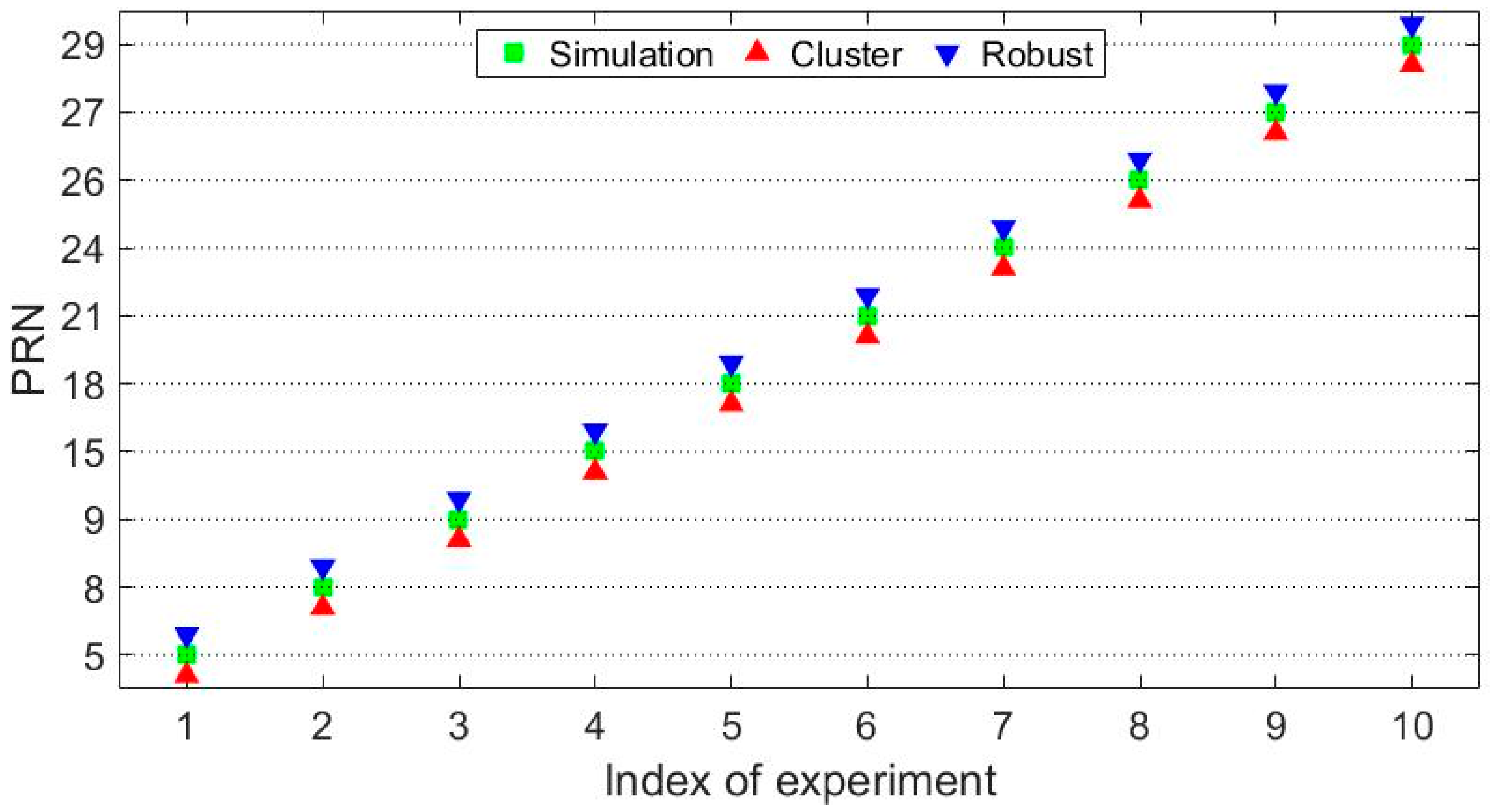
In this section, we analyze the performance of the two methods at a specific epoch when there were various numbers of cycle slips. First, we simulated a small cycle slip with size of one cycle on one satellite at a time and detected cycle slips using both the proposed method and the current robust estimation method. Ten satellites were available at the 100th epoch, and each had a simulated cycle slip, in turn. The detection results with methods I and II are shown in
Figure 3. The horizontal axis shows the index of the experiment, and the vertical axis shows the available satellites. The green squares denote simulated cycle slips. The blue inverted triangles denote detection results with the robust estimation method and the red triangles represent detected cycle slips using the proposed method. We can see that both methods performed well when there was only one simulated cycle slip at a time. Hence, the proposed method can be preliminarily concluded to be effective.
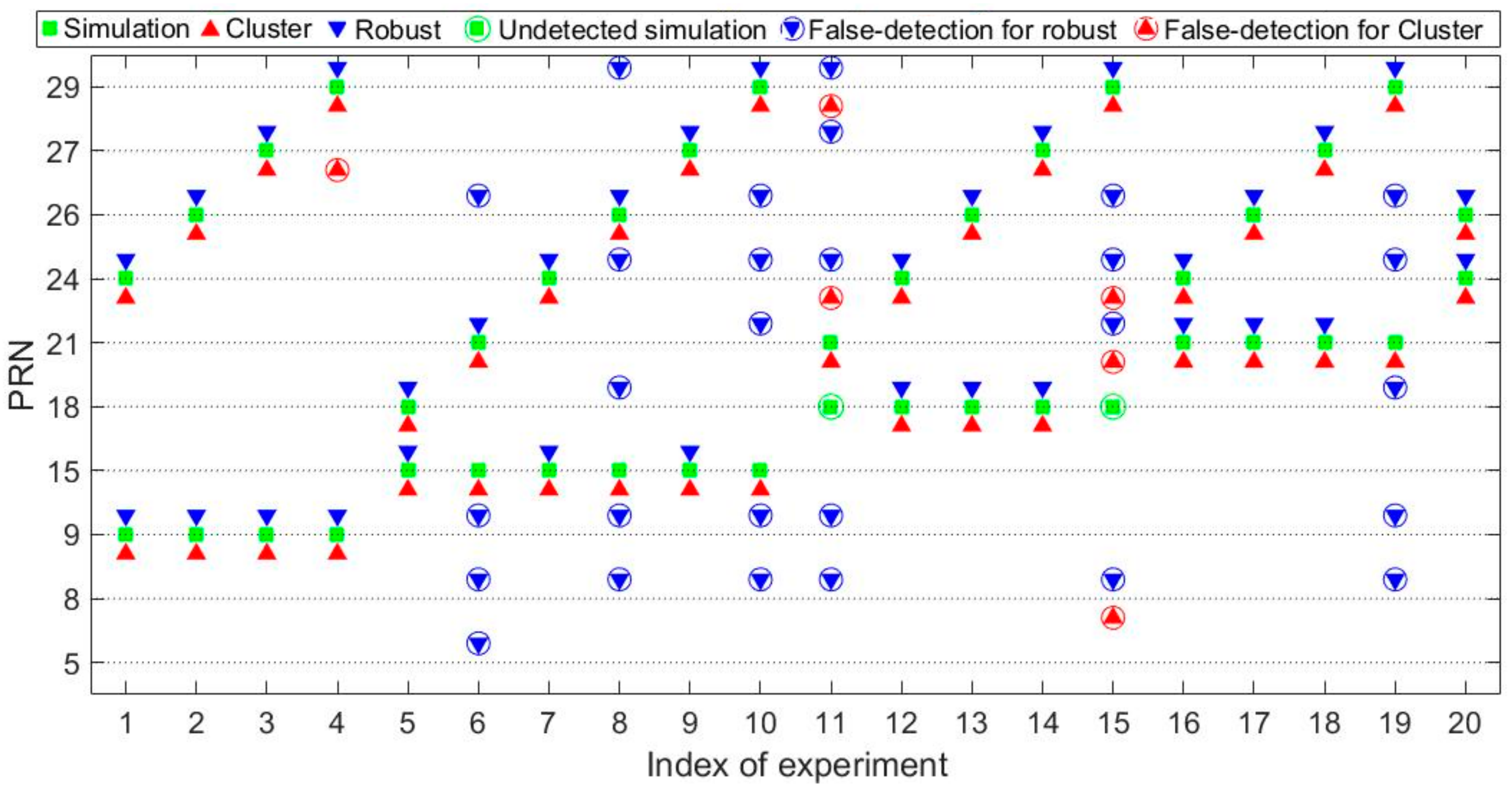
We further simulated cycle slips on two satellites at a time. The size of simulated cycle slip is one cycle for each satellite. There are 45 ways to select two satellites from ten. We randomly chose 20 of them. All detection results with both methods are presented in
Figure 4. The symbols are the same as above. In addition, the simulated cycle slips that were not successfully detected are also individually marked with green circles and the detected but not simulated cycle slips are marked with blue circles for robust estimation method while red circles for the proposed method.
We can see from
Figure 4 that better performance can be obtained with the proposed method. For all experiments, seven simulated cycle slips could not be detected with the robust estimation method, and five of those were correctly detected with the proposed method. Also, the proposed method obviously had lower false-alarm rates. Some satellites without simulated cycle slips were thought to have cycle slips using the robust estimation method, but most of these cases were avoided with the proposed method. Statistical results are shown in
Table 2.
As shown in
Table 2, for all experiments, a total of 40 cycle slips were simulated. A total of 61 cycle slips were detected for the robust estimation method and 44 for the fuzzy-cluster-based method. Among all detections, methods I and II correctly detected 33 and 38, respectively, that is, the correct-detection rate was 54.1% for the robust estimation method and 86.4% using the proposed method. The undetection rate was 17.5% for robust estimation and 5% using the fuzzy-cluster-based method. In addition, the false-detection rate reached 45.9% for the robust method while 13.6% for the proposed method.
Overall, in a single epoch, the proposed method performed as well as the robust estimation method when there was only one simulated cycle slip at a time. When the number of cycle slips increased to two, better performance was obtained using the fuzzy-cluster-based method, with a higher correct-detection rate and lower undetection rate.
3.3. Performance of Multi-Epoch Cycle-Slip Detection
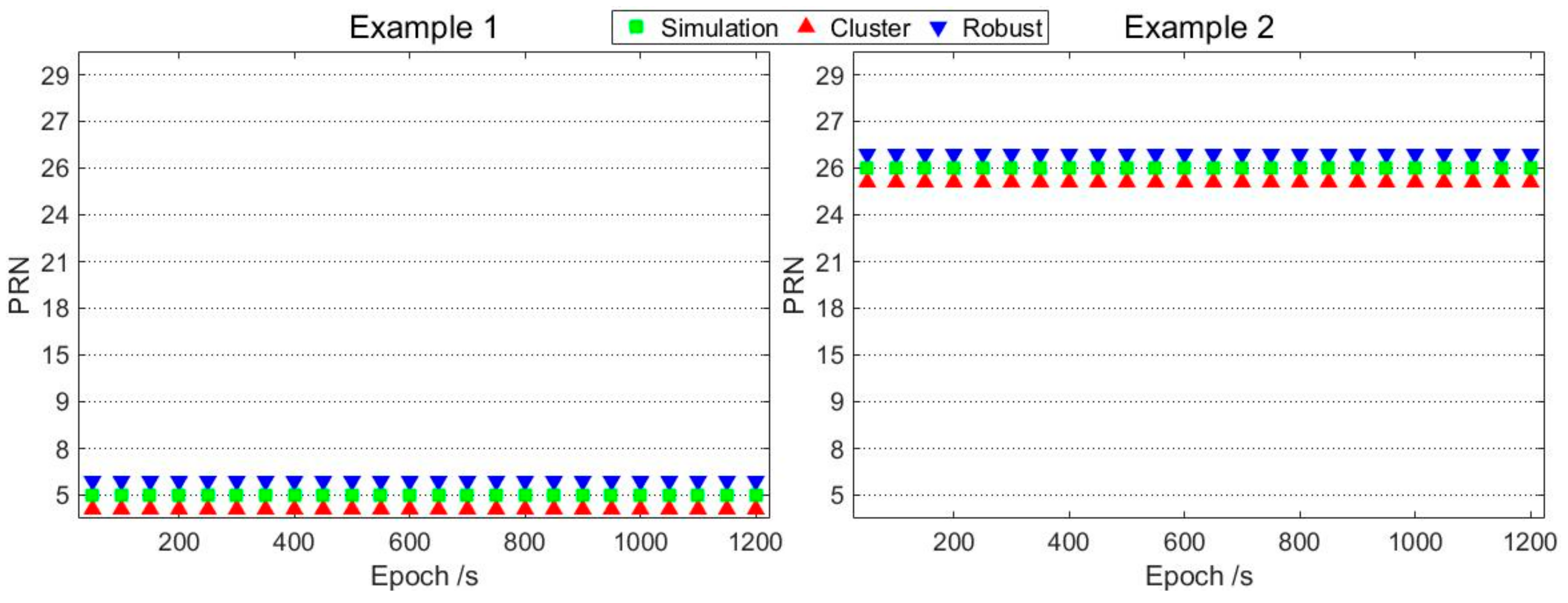
We performed the same experiments for multi-epochs instead of only one epoch and determined whether the conclusion drawn above was reasonable. The size of simulated cycle slip is one cycle for each satellite. To be more specific, cycle slips were first simulated on one satellite every 50 epochs to be detected using both two methods. Similarly, there are 10 ways to select one satellite from ten satellites and all possible experiments were performed. Two examples are shown below.
As shown in
Figure 5, the left panel describes the performance of the two methods when cycle slips were simulated on satellite G05 every 50 epochs, and the right panel is for satellite G26. Both methods could correctly detect all simulated cycle slips at multi-epochs. Experiments were conducted on 10 available satellites in turn, and statistical results are presented in
Table 3. We can see that a total of 240 simulated cycle slips were correctly detected, with a correct-detection rate of 100% for both methods.
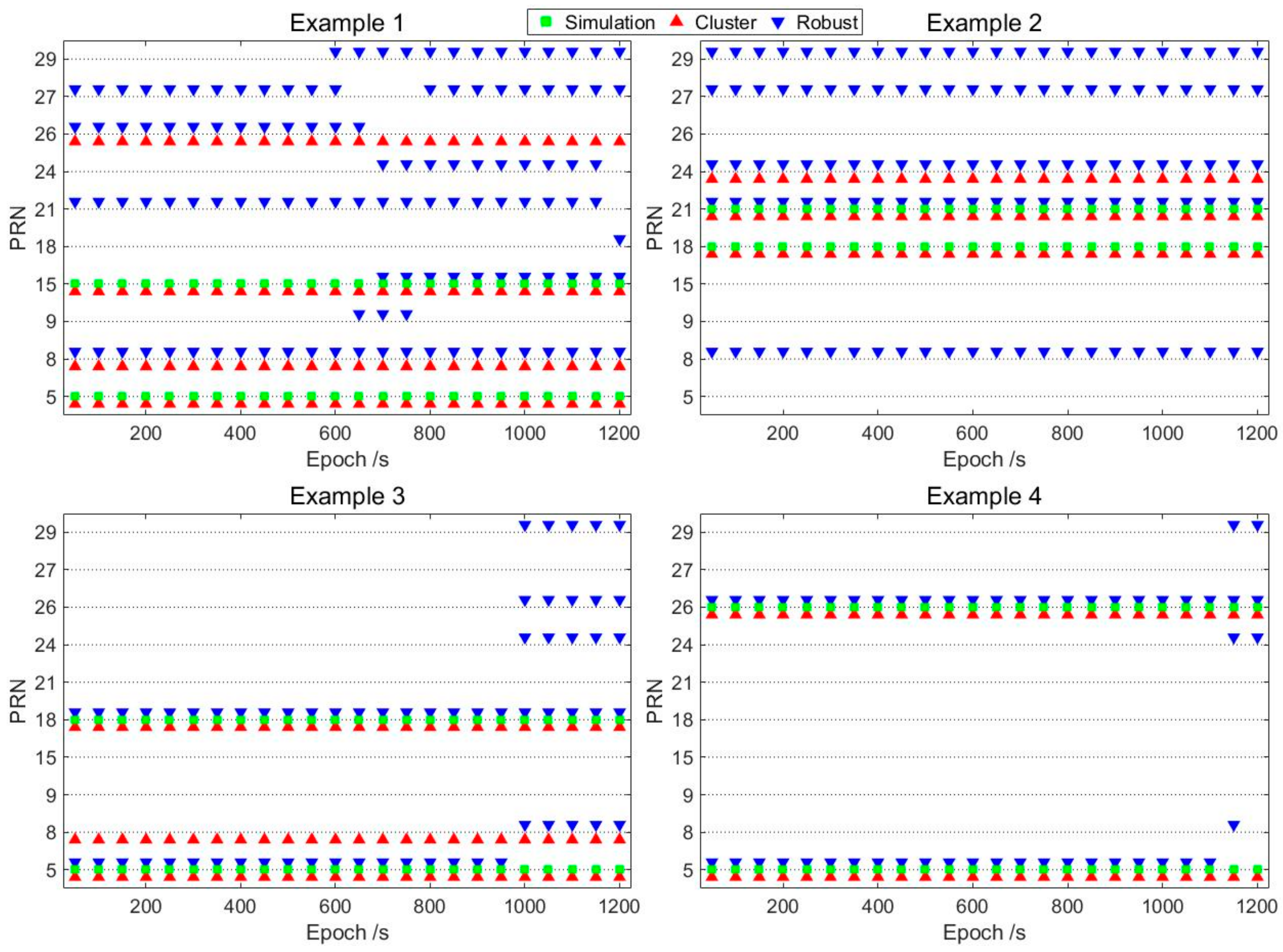
Afterwards, cycle slips were simulated on two satellites at a time every 50 epochs, and the performance of the two methods was compared. There are 45 ways to select two satellites from ten satellites. Some typical examples are shown in
Figure 6. Example 1 describes the detection results when cycle slips were simulated on satellites G05 and G15 simultaneously. Example 2 is for satellites G18 and G21, Example 3 is for satellites G05 and G18, and Example 4 is for satellites G05 and G26.
As shown in Examples 3 and 4, almost all cycle slips were correctly detected with both methods. However, from Examples 1 and 2, we can see that nearly half of the simulated cycle slips were not successfully detected with the robust estimation method, while the fuzzy-cluster-based method detected almost all cycle slips correctly. Statistical results for the four examples are shown in
Table 4.
We can observe that in Examples 1 and 2, the correct-detection rate was below 30% using the robust estimation method and was more than 50% with the fuzzy-cluster method. The undetection rate exceeded 25% using method I and was zero with method II. The false-detection was more than 70% for the robust method while below 50% for the proposed method. In Example 3, two methods showed essentially identical correct-detection rates and false-detection rate, but the undetection rate with the fuzzy-cluster-based method was zero, while it reached 10% with robust estimation. In Example 4, the fuzzy-cluster-based method still performed better than the robust estimation method, with a higher correct-detection rate and lower undetection and false-detection rate. To more comprehensively evaluate the performance of the proposed method, we conducted 45 experiments, covering all possible choices, when selecting two from ten satellites. The statistical results are shown in
Table 5.
As shown in
Table 5, a total of 2160 cycle slips were simulated in all experiments. The correct-detection rate was only 51.9% using the robust estimation method, while it reached 84.3% with the fuzzy-cluster method. The false-detection rate reached about 50% for the robust method and only about 15% for the fuzzy-cluster method. Moreover, the undetection rate was 13.9% with the robust estimation method, and only 3.1% with the proposed method. Therefore, we can conclude that the fuzzy-cluster method outperformed the robust estimation method, with a higher correct-detection rate and a lower undetection rate.
3.4. Performance of Multi-Cycle-Slip Detection
We computed the correct-detection rate and undetection rate when cycle slips were simulated on various numbers of satellites. Considering the average number of visible GPS satellites is about 9–10, and at least four satellites are required to positioning (
http://www.csno-tarc.cn/gps/number), we assumed that at most five satellites suffered from cycle slips, hence five situations were considered. In these five situations, the number of satellites suffering from cycle slips was set in turn from 1 to 5. Over the collected 1200 seconds, cycle slips were simulated every 50 epochs on the selected satellites in each situation. It should be noted that there are many choices when selecting a specified number of satellites from ten available satellites. For example, there are 10 ways when selecting one satellite from ten satellites and 45 choices when selecting two from ten satellites. We took all possible choices into account to ensure reliable statistical results, which are presented in
Figure 7. The horizontal axis indicates the number of satellites where cycle slips were simulated, and the vertical axis expresses the correct-detection and undetection rates as percentages. The blue line shows the results with the robust estimation method, and the red line is for the fuzzy-cluster method. The diamonds denote the correct-detection rate, and the circles denote the undetection rate.
We can see that the correct-detection rate decreased with an increased number of satellites simulated with cycle slips for both methods, but to different extents. The correct-detection rate rapidly declined to below 50% when the number of satellites simulated with cycle slips was larger than 2 using the robust estimation method. However, with the proposed method, it remained at more than 60% even when the number of satellites simulated with cycle slips reached 5. In addition, the undetection rate had a rising trend with different amplitudes for the two methods when the number of satellites simulated with cycle slips increased. For the robust method, this rate quickly exceeded 30% when the number of satellites simulated with cycle slips increased to 3. It was already more than 60% when the number of satellites simulated with cycle slips was 5. But, using the proposed method, the rate remained lower than 30% even if the number of satellites simulated with cycle slips reached 5. Overall, the proposed method outperformed the current robust estimation method, with a higher correct-detection rate and lower undetection rate.
3.5. Performance of Different Amplitudes of Cycle-Slip
All of the experiments above are conducted with simulated cycle slip of one cycle. We further evaluate the performance of the proposed method under the situation of different amplitudes of cycle slip. Two cases are considered. The first one is simulating different amplitudes of cycle slip at the same time on more than one satellites. As mentioned above, we assume that at most five satellites suffer from cycle slip at the same time. So, in this case, four experiments are designed as follows: at the 100th epoch, different amplitudes of cycle slip are simulated on arbitrary two satellites, three satellites, four satellites, and five satellites respectively. The simulation and detection results with two methods are shown in
Table 6.
As shown in
Table 6, when cycle slips with size of 1 cycle and 5 cycles are simulated on satellites G05 and G15 respectively, they can be successfully detected with the correct-detection rate of 67% for robust method while 100% for the proposed method. When cycle slips with size of 1 cycle, 5 cycles, and 10 cycles are simulated on satellites G05, G18, and G21 respectively, the correct-detection rate declines to 40% for the robust method while it keeps 75% for the cluster method. Meanwhile, the un-detection rate reaches to 34% for the robust method while 0% for the cluster method. When four or five different amplitudes of cycle slips are simulated on four or five satellites respectively, the correct-detection rate is below than 40% for the robust method while keeps 60% for the cluster method. In addition, the undetection rate is more than 50% for the robust method and lower than 40% for the cluster method.
The other case is simulating different amplitudes of cycle slip at different epochs on one satellite. We randomly choose one satellite G05 and simulated cycle slips every 50 epochs. The size of simulated cycle slips is set from 1 to 240 cycles for various epochs. The simulation and detection results with two methods are shown in
Table 7. We can see that all simulated cycle slips with different amplitudes can be successfully detected with both two methods.
4. Discussion
The results above indicate that the proposed method outperforms the robust estimation method, with a higher correct-detection rate and lower undetection rate. As the number of satellites simulated with cycle slips increases, the correct-detection rate rapidly decreases from 100% to below 50% with the robust estimation method. While the correct-detection rate using the proposed method is always more than 60%, even if the number of satellites simulated with cycle slips reaches five. In addition, the proposed method always has a lower undetection rate than the robust estimation method.
It should be point out that this new method succeeds with conditions. The data used for tests were recorded at a high rate 1.0 Hz and not under high ionospheric activity. The variations of tropospheric and ionospheric delay between epochs can be ignored in this paper.
In addition, although the better performance have been achieved, there are still much work to be done in the further to modify this method. For example, various cluster algorithms can obtain different cluster results. Integration of pseudorange observations or multi-frequency or multi-system may also effect the cluster results. A better cluster results may improve the correct-detection rate and reduce the undetection rate. Additionally, the efficiency of this method should also be evaluated to adapt to real-time application.
Moreover, the effect of this method on positioning could be analyzed in the next work. As we all know, the higher the undetection rate, the worse the positioning accuracy. Meanwhile, the higher the false-detection rate, the more frequent initialization and the longer convergence time. So we will analyze its impact on positioning from these two aspects in the near further.
5. Conclusions
We propose a new fuzzy-cluster-based cycle-slip detection method for GPS single-frequency signals. In this method, the epoch when cycle slips occur is first determined by a chi-square test. Afterwards, the satellite suffering from cycle slip is identified based on fuzzy-cluster algorithm. This algorithm makes full use of a posteriori standard errors and the design matrix, and is characterized by a high correct-detection rate and low undetection rate.
To evaluate the proposed method, we compared it with the current robust estimation method using some simulation studies based on real GPS L1 measurements. Results indicated that the proposed method outperformed the current robust estimation method, with a higher correct-detection rate and lower undetection rate. Specifically, when the number of satellites simulated with cycle slips increased to two, the correct-detection rate rapidly declined from 100% to below 50% using the robust estimation method, while with the proposed method, the percentage was always more than 60 even if the number of satellites simulated with cycle slips reached five. The undetection rate increased to more than 30% when the number of satellites simulated with cycle slips was larger than three, and its maximum was nearly 70% for the robust estimation method. However, the maximum percentage for the proposed method was lower than 30, even if the number of satellites simulated with cycle slips increased to five.
In conclusion, the proposed method can perform well, with a higher correct-detection rate and lower false-alarm rate. In addition, this method can be applied to dual-frequency, triple-frequency, and even multi-systems. Its effect on these situations can be further analyzed. Moreover, different clustering algorithms may have various results. Thus, an enhanced or modified cluster algorithm and its effect on cycle-slip detection can be explored in the near future.
Author Contributions
Z.L. and M.L. conceived and designed the experiment; Z.L. performed the experiment, analyzed the result and wrote the first draft, C.S., M.L., C.D., and L.C. reviewed and revised the manuscript; W.S., R.L. and P.Z. helped with the writing of the text.
Funding
This research is funded by the National Key Research and Development Plan (Grant No. 2016YFB0501802), the National Natural Science Foundation (Grant No. 41574027, 41774035 and 41574030), the Wuhan Morning Light Plan of Youth Science and Technology (Grant No. 2017050304010301), and Shanxi Key Laboratory of Integrated and Intelligent Navigation (SKLIIN-20180202).
Acknowledgments
We would also like to acknowledge the PANDA software developed by GNSS Research Center of Wuhan University. We appreciate the editor and anonymous reviewers for their valuable comments and improvements to this manuscript.
Conflicts of Interest
The authors declare no conflict of interest.
References
- Marques, H.A.; Marques, H.A.S.; Aquino, M.; Veettil, S.V.; Monico, J.F.G. Accuracy assessment of Precise Point Positioning with multi-constellation GNSS data under ionospheric scintillation effects. J. Space Weather Space Clim. 2018, 8, A15. [Google Scholar] [CrossRef]
- Prikryl, P.; Jayachandran, P.T.; Mushini, S.C.; Pokhotelov, D.; MacDougall, J.W.; Donovan, E.; Spanswick, E.; Maurice, J.-P.S. GPS TEC, scintillation and cycle slips observed at high latitudes during solar minimum. Ann. Geophys. 2010, 28, 1307–1316. [Google Scholar] [CrossRef]
- Yu, Y.; Astafyeva, E.; Padokhin, A.; Ivanova, V.; Syrovatskii, S.; Podlesnyi, A. The 6 September 2017 X-Class Solar Flares and Their Impacts on the Ionosphere, GNSS and HF Radio Wave Propagation. Space Weather 2018, 16, 1013–1027. [Google Scholar] [CrossRef]
- Blewitt, G. An automatic editing algorithm for GPS data. Geophys. Res. Lett. 1990, 17, 199–202. [Google Scholar] [CrossRef]
- Hatch, R. The Synergism of GPS Code and Carrier Measurements. In Proceedings of the 3rd International Geodetic Symposium on Satellite Doppler Positioning, Las Cruces, NM, USA, 8–12 February 1982; pp. 1213–1231. [Google Scholar]
- Melbourne, W.G. The Case for Ranging in GPS Based Geodetic Systems. In Proceedings of the 1st International Symposium on Precise Positioning with the Global Positioning System, Rockville, ML, USA, 15–19 April 1985; pp. 373–386. [Google Scholar]
- Wübbena, G. Software Developments for Geodetic Positioning with GPS Using TI 4100 Code and Carrier Measurements. In Proceedings of the 1st International Symposium on Precise Positioning with the Global Positioning System, Rockville, ML, USA, 15–19 April 1985; pp. 403–412. [Google Scholar]
- Li, B.; Qin, Y.; Li, Z.; Lou, L. Undifferenced cycle slip estimation of triple-frequency BeiDou signals with ionosphere prediction. Mar. Geod. 2016, 39, 348–365. [Google Scholar] [CrossRef]
- Zhao, Q.; Sun, B.; Dai, Z.; Hu, Z.; Shi, C.; Liu, J. Real-time detection and repair of cycle slips in triple-frequency GNSS measurements. GPS Solut. 2015, 19, 381–391. [Google Scholar] [CrossRef]
- De Lacy, M.C.; Reguzzoni, M.; Sanso, F. Real-time cycle slip detection in triple-frequency GNSS. GPS Solut. 2012, 16, 353–362. [Google Scholar] [CrossRef]
- Schönemann, E.; Becker, M.; Springer, T. A new approach for GNSS analysis in a multi-GNSS and multi-signal environment. J. Geod. Sci. 2011, 1, 204–214. [Google Scholar] [CrossRef]
- Chen, J.; Zhang, Y.; Wang, J.; Yang, S.; Dong, D.; Wang, J.; Qu, W.; Wu, B. A simplified and unified model of multi-GNSS precise point positioning. Adv. Space Res. 2015, 55, 125–134. [Google Scholar] [CrossRef]
- Feng, Y.; Gu, S.; Shi, C.; Rizos, C. A reference station-based GNSS computing mode to support unified precise point positioning and real-time kinematic services. J. Geod. 2013, 87, 945–960. [Google Scholar] [CrossRef]
- Odijk, D.; Zhang, B.; Khodabandeh, A.; Odolinski, R.; Teunissen, P.J. On the estimability of parameters in undifferenced, uncombined GNSS network and PPP-RTK user models by means of S-system theory. J. Geod. 2016, 90, 15–44. [Google Scholar] [CrossRef]
- Lichtenegger, H.; Hofmann, W.B. GPS-Data Preprocessing for Cycle-Slip Detection. In Global Positioning System: An Overview; Springer: New York, NY, USA, 1990. [Google Scholar]
- Kleusberg, A.; Georgiadou, Y.; van den, H.F.; Héroux, P. GPS Data Preprocessing with DIPOP 3.0; Internal Technical Memorandum, Department of Surveying Engineering, University of New Brunswick: Fredericton, NB, Canada, 1993. [Google Scholar]
- Baarda, W. A Testing Procedure for Use in Geodetic Networks; Delft Kanaalweg Rijkscommissie Voor Geodesie, Netherlands Gedetic Commission: Delft, The Netherlands, 2013; p. 1. [Google Scholar]
- Teunissen, P.J.G. Testing Theory an Introduction Series on Mathematical Geodesy and Positioning; Delft University Press: Washington, DC, USA, 2000. [Google Scholar]
- Teunissen, P.J.G.; Simons, D.G.; Tiberius, C.C.J.M. Probability and Observation Theory; Delft University of Technology: Delft, The Netherlands, 2005. [Google Scholar]
- Lacy, D.; Reguzzoni, M.; Fernando, S.; Venuti, G. The bayesian detection of discontinuities in a polynomial regression and its application to the cycle-slip problem. J. Geod. 2008, 82, 527–542. [Google Scholar] [CrossRef]
- Zhang, Q.; Gui, Q. Bayesian methods for outliers detection in gnss time series. J. Geod. 2013, 87, 609–627. [Google Scholar]
- Song, W.; Yao, Y. Pre-process strategy in complex movement using single-frequency GPS data. Geomat. Inf. Sci. Wuhan Univ. 2009, 34, 1005–1008. [Google Scholar]
- Kirkkojaakkola, M.; Traugott, J.; Odijk, D.; Collin, J.; Sachs, G.; Holzapfel, F. A Raim Approach to GNSS Outlier and Cycle Slip Detection using L1 Carrier Phase Time-Differences. In Proceedings of the IEEE Workshop on Signal Processing Systems, Tampere, Finland, 7–9 October 2009; pp. 273–278. [Google Scholar]
- Seigo, F.; Susumu, S.; Takayuki, Y. Cycle slip detection and correction methods with time-differenced model for single frequency gnss applications. Trans. Inst. Syst. Control Inf. Eng. 2013, 26, 8–15. [Google Scholar]
- Teunissen, P.J.G.; Bakker, P.F.D. Single-receiver single-channel multi-frequency gnss integrity: Outliers, slips, and ionospheric disturbances. J. Geod. 2013, 87, 161–177. [Google Scholar] [CrossRef]
- Zangeneh-Nejad, F.; Amiri-Simkooei, A.R.; Sharifi, M.A.; Asgari, J. Cycle slip detection and repair of undifferenced single-frequency gps carrier phase observations. GPS Solut. 2017, 21, 1593–1603. [Google Scholar] [CrossRef]
- Li, T.; Melachroinos, S. An enhanced cycle slip repair algorithm for real-time multi-gnss, multi-frequency data processing. GPS Solut. 2019, 23, 1. [Google Scholar] [CrossRef]
- Bezdek, J.C. Pattern recognition with fuzzy objective function algorithms. Adv. Appl. Pattern Recognit. 1981, 22, 203–239. [Google Scholar]
- Bezdek, J.C.; Ehrlich, R.; Full, W. Fcm: The fuzzy c-means clustering algorithm. Comput. Geosci. 1984, 10, 191–203. [Google Scholar] [CrossRef]
- Bruzzone, L.; Diego, F.P. An adaptive semiparametric and context-based approach to unsupervised change detection in multitemporal remote-sensing images. IEEE Trans. Image Process. A Publ. IEEE Signal Process. Soc. 2002, 11, 452–466. [Google Scholar] [CrossRef]
- Höppner, F.; Klawonn, F.; Kruse, R.; Runkler, T. Fuzzy Cluster Analysis: Methods for Classification, Data Analysis and Image Recognition; John Wiley: New York, NY, USA, 1999. [Google Scholar]
- Kaufman, L.; Rousseeuw, P.J. Finding groups in data: An introduction to cluster analysis. J. Am. Stat. Assoc. 1990, 508, 314–327. [Google Scholar]
- Kitamura, D.; Saruwatari, H.; Kameoka, H.; Takahashi, Y.; Kondo, K.; Naka, S. Multichannel signal separation combining directional clustering and nonnegative matrix factorization with spectrogram restoration. IEEE/ACM Trans. Audio Speechlang. Process. 2015, 23, 654–669. [Google Scholar] [CrossRef]
- Remondi, B.W. Global positioning system carrier phase: Description and use. Bull. Geod. 1985, 59, 361–377. [Google Scholar] [CrossRef]
- Householder, A.S. Unitary Triangularization of a Nonsymmetric Matrix. J. ACM 1958, 5, 339–342. [Google Scholar] [CrossRef]
- Hewitson, S.; Wang, J. Gnss receiver autonomous integrity monitoring (raim) performance analysis. GPS Solut. 2006, 10, 155–170. [Google Scholar] [CrossRef]
- Petit, G.; Luzum, B. IERS Conventions 2010; No. 36 in IERS Technical Note; Verlag des Bundesamts für Kartographie und Geodäsie: Frankfurt am Main, Germany, 2010. [Google Scholar]
- Freda, P.; Angrisano, A.; Gaglione, S.; Troisi, S. Time-differenced carrier phases technique for precise GNSS velocity estimation. GPS Solut. 2015, 19, 335–341. [Google Scholar] [CrossRef]
Figure 1.
The upper panel is the 2-nd order differences of phase observation series. Subfigure (a) is the 2-nd order differences of phase observation series without cycle slip and subfigure (b) is the one with cycle slip. The below panel is the standard deviation series. The left subfigure (c) is the standard deviation series without cycle slip and the right subfigure (d) is the one with cycle slip.
Figure 2.
Flow chart of the fuzzy-cluster-based method for cycle-slip detection.
Figure 2.
Flow chart of the fuzzy-cluster-based method for cycle-slip detection.
Figure 3.
Cycle-slip detection results with methods I and II at the 100th epoch when cycle slip was simulated on one satellite at a time. Blue inverted triangles denote detection results with robust estimation method; red triangles are for the fuzzy-cluster-based method. Green squares denote simulated cycle slips. Ten satellites were available at this epoch and each satellite has a simulated cycle slip in turn. The horizontal axis denotes the index of each experiment, and the vertical axis shows available satellites. All simulated cycle slips could be correctly detected with both two methods.
Figure 4.
Cycle-slip detection results with methods I and II when cycle slips were simulated on two satellites at a time. The blue inverted triangles denote the detection results with the robust estimation method, while the red triangles are for the fuzzy-cluster-based method. Green squares denote simulated cycle slips. Green circles denote the simulated cycle slips that were not successfully detected; blue circles denote the detected but not simulated cycle slips for method I and red circles for method II. The figure shows 20 from all possible experiments. The horizontal axis shows the index of each experiment, and the vertical axis shows the available satellites.
Figure 5.
Cycle-slip detection results with methods I and II over 1200 seconds when cycle slips were simulated on one satellite every 50 epochs. The left panel Example 1 is for G05, and the right panel Example 2 for G26. The blue inverted triangles are the detection results with the robust estimation method, while the red triangles are for the fuzzy-cluster-based method. The green squares denote simulated cycle slips. All simulated cycle slips could be correctly detected with both two methods.
Figure 6.
Cycle-slip detection results using methods I and II over 1200 seconds when cycle slips were simulated on two satellites at a time every 50 epochs. Blue inverted triangles denote detection results with the robust estimation method, and red triangles are for the fuzzy-cluster-based method. Green squares denote simulated cycle slips. Example 1 shows the detection results when cycle slips were simulated on G05 and G15, Example 2 is for G18 and G21, Example 3 is for G05 and G18, and Example 4 is for G05 and G26. Almost all simulated cycle slips were correctly detected with the fuzzy-cluster-based method, but some were not detected with the robust estimation method.
Figure 7.
Correct-detection rate (diamonds) and undetection rate (circles) when various numbers of satellites were simulated with cycle slips for the robust estimation method (blue lines) and fuzzy-cluster-based method (red lines).
Figure 7.
Correct-detection rate (diamonds) and undetection rate (circles) when various numbers of satellites were simulated with cycle slips for the robust estimation method (blue lines) and fuzzy-cluster-based method (red lines).
Table 1.
Data processing strategy and observation model used during cycle-slip detection in precise point positioning (PPP).
Table 1.
Data processing strategy and observation model used during cycle-slip detection in precise point positioning (PPP).
| Item | Contents |
|---|
| Models | Observables | Single-differenced phase measurement: GPS L1
Original measurement noise: 3 mm |
| Sampling rate | 1 s |
| Cut-off elevation | 7° |
| Weighting | Elevation-dependent, 1 for E > 30°, otherwise 2sin(E) |
| Tropospheric delay | GMF, a priori model |
| Station phase center | Igs08.atx |
| Satellite phase center | Igs08.atx |
| Relativity effect | IERS Conventions 2010 [37] |
| Station displacement | Solid Earth tide, pole tide, ocean loading tide |
| Phase windup | Corrected |
| Parameters estimated in cycle-slip detection | Station coordinates variation between epochs | Estimated with LSQ |
| Receiver clock variation between epochs | Estimated with LSQ |
| Ambiguity variation between epochs | Considered as 0 in the same arc but cycle slips for different arc |
| Tropospheric variation between epochs | ignored for 1 s data [38] |
| Ionospheric variation between epochs | ignored for 1 s data [38] |
Table 2.
Statistical results of cycle-slip detection when cycle slips were simulated on two satellites at a time, using robust estimation and clustering analysis method.
Table 2.
Statistical results of cycle-slip detection when cycle slips were simulated on two satellites at a time, using robust estimation and clustering analysis method.
| Type of Cycle Slip | Robust | Cluster |
|---|
| Simulation | 40 | 40 |
| Detection | 61 | 44 |
| Correct Detection | 33 | 38 |
| Correct-Detection rate | 33/61 = 54.1% | 38/44 = 86.4% |
| False-Detection rate | (61−33)/61 = 45.9% | (44−38)/44 = 13.6% |
| Undetection rate | (40−33)/40 = 17.5% | (40−38)/40 = 5.0% |
Table 3.
Statistical cycle-slip detection results on multi-epochs when the cycle slip was simulated on one satellite at a time using the robust estimation method and proposed method.
Table 3.
Statistical cycle-slip detection results on multi-epochs when the cycle slip was simulated on one satellite at a time using the robust estimation method and proposed method.
| Type of Cycle Slip | Robust | Cluster |
|---|
| Simulation | 240 | 240 |
| Detection | 240 | 240 |
| Correct Detection | 240 | 240 |
| Correct-Detection rate | 100% | 100% |
| False-Detection rate | 0% | 0% |
| Undetection rate | 0% | 0% |
Table 4.
Statistical cycle-slip-detection results for the four typical examples when cycle slips were simulated on two satellites. I denotes the robust estimation method and II is the fuzzy-cluster-based method.
Table 4.
Statistical cycle-slip-detection results for the four typical examples when cycle slips were simulated on two satellites. I denotes the robust estimation method and II is the fuzzy-cluster-based method.
| Type of Cycle Slip | Example 1 | Example 2 | Example 3 | Example 4 |
|---|
| I | II | I | II | I | II | I | II |
|---|
| Simulation | 48 | 48 | 48 | 48 | 48 | 48 | 48 | 48 |
| Detection | 119 | 96 | 120 | 72 | 63 | 72 | 51 | 48 |
| Correct Detection | 35 | 48 | 24 | 48 | 43 | 48 | 46 | 48 |
| Correct-Detection rate | 29% | 50% | 20% | 67% | 68% | 67% | 90% | 100% |
| False-Detection rate | 71% | 50% | 80% | 33% | 32% | 33% | 10% | 0% |
| Undetection rate | 27% | 0% | 50% | 0% | 10% | 0% | 4% | 0% |
Table 5.
Statistical cycle-slip detection results on multi-epochs for all possible experiments when cycle slips were simulated on two of 10 satellites at a time, using robust estimation and the fuzzy-cluster method.
Table 5.
Statistical cycle-slip detection results on multi-epochs for all possible experiments when cycle slips were simulated on two of 10 satellites at a time, using robust estimation and the fuzzy-cluster method.
| Type of Cycle Slip | Robust | Cluster |
|---|
| Simulation | 2160 | 2160 |
| Detection | 3574 | 2549 |
| Correct Detection | 1858 | 2092 |
| Correct-Detection rate | 51.9% | 84.3% |
| False-Detection rate | 49.1% | 15.7% |
| Undetection rate | 13.9% | 3.1% |
Table 6.
Statistical cycle-slip-detection results for the four cases when different amplitudes of cycle slips were simulated on two, three, four, or five satellites. I denotes the robust estimation method and II is the fuzzy-cluster-based method.
Table 6.
Statistical cycle-slip-detection results for the four cases when different amplitudes of cycle slips were simulated on two, three, four, or five satellites. I denotes the robust estimation method and II is the fuzzy-cluster-based method.
| Type of Cycle Slip | G05,G15
(1,5) | G05,G18,G21
(1,5,10) | G05,G15,G18,G21
(1,5,10,20) | G05,G15,G18,G21,G26
(1,5,10,20,30) |
|---|
| I | II | I | II | I | II | I | II |
|---|
| Simulation | 2 | 2 | 3 | 3 | 4 | 4 | 5 | 5 |
| Detection | 3 | 2 | 5 | 4 | 6 | 5 | 6 | 5 |
| Correct Detection | 2 | 2 | 2 | 3 | 2 | 3 | 2 | 3 |
| Correct-Detection rate | 67% | 100% | 40% | 75% | 34% | 60% | 34% | 60% |
| False-Detection rate | 33% | 0% | 60% | 25% | 66% | 40% | 66% | 40% |
| Undetection rate | 0% | 0% | 34% | 0% | 50% | 25% | 60% | 40% |
Table 7.
Statistical cycle-slip detection results on multi-epochs when the different amplitudes of cycle slips were simulated on satellite G05 using the robust estimation method and proposed method.
Table 7.
Statistical cycle-slip detection results on multi-epochs when the different amplitudes of cycle slips were simulated on satellite G05 using the robust estimation method and proposed method.
| Type of Cycle Slip | Robust | Cluster |
|---|
| Simulation | 240 | 240 |
| Detection | 240 | 240 |
| Correct Detection | 240 | 240 |
| Correct-Detection rate | 100% | 100% |
| False-Detection rate | 0% | 0% |
| Undetection rate | 0% | 0% |
© 2019 by the authors. Licensee MDPI, Basel, Switzerland. This article is an open access article distributed under the terms and conditions of the Creative Commons Attribution (CC BY) license (http://creativecommons.org/licenses/by/4.0/).


 ,
, 


