Sparse Unmixing for Hyperspectral Image with Nonlocal Low-Rank Prior

Abstract

Hyperspectral unmixing is a key preprocessing technique for hyperspectral image analysis. To further improve the unmixing performance, in this paper, a nonlocal low-rank prior associated with spatial smoothness and spectral collaborative sparsity are integrated together for unmixing the hyperspectral data. The proposed method is based on a fact that hyperspectral images have self-similarity in nonlocal sense and smoothness in local sense. To explore the spatial self-similarity, nonlocal cubic patches are grouped together to compose a low-rank matrix. Then, based on the linear mixed model framework, the nuclear norm is constrained to the abundance matrix of these similar patches to enforce low-rank property. In addition, the local spatial information and spectral characteristic are also taken into account by introducing TV regularization and collaborative sparse terms, respectively. Finally, the results of the experiments on two simulated data sets and two real data sets show that the proposed algorithm produces better performance than other state-of-the-art algorithms.

1. Introduction

Hyperspectral remote sensing generally uses an imaging spectrometer to collect spatial and spectral information. Hyperspectral images can obtain tens or even hundreds of consecutive narrow-band information (generally less than 10 nm) of each pixel in a spectral domain, and each pixel can extract a continuous spectral curve [1]. Therefore, hyperspectral images have the property of high spectral resolution, which greatly improves the ability to detect the property of the material. It has been actively discussed by researchers and widely applied in many fields, such as agricultural production, geological survey, urban planning, and environmental monitoring [2,3]. However, because of the limitations of optical instrument’s performance and imperfect spectral acquisition techniques, the spatial resolution of hyperspectral images is low, which results in a pixel that may contain more than one type of ground object signature, called a mixed pixel [4,5]. Because of the existence of many mixed pixels, the accuracy of hyperspectral image processing has been greatly affected. Therefore, hyperspectral unmixing is a key preprocessing technique for hyperspectral image analysis.

The goal of hyperspectral unmixing is to extract the pure spectral signatures (called endmembers) in the scene [6] at first and then estimate the corresponding proportions (called abundances) of these endmembers [7]. There are two main models of hyperspectral unmixing: linear mixture model (LMM) [8,9] and nonlinear mixture model (NLMM) [10,11,12]. Different from the NLMM, the LMM has the advantages of simplicity, high efficiency, and clear physical meaning. The LMM also can describe better the actual spectral mixing phenomenon of hyperspectral images with spatial resolution under the meter level. Therefore, the LMM is applied for hyperspectral unmixing widely and it assumes that the observed spectral signal of each mixed pixel can be approximated as a linear mixture of all pure endmembers in that pixel.

With the LMM, there are many endmember extraction algorithms based on the statistical and geometry methods that have been proposed for hyperspectral images, such as the vertex component analysis (VCA) [13], pixel purity index [14], and N-FINDR [15] algorithms. These algorithms only require a small amount of prior knowledge of the hyperspectral image. Nevertheless, they need the assumption of pure pixel’s existence in the scene, which does not hold in many datasets. Thus, some researchers proposed algorithms that do not require this assumption, such as minimum volume simplex analysis (MVSA) [16] and iterative constrained endmembers (ICE) [17]. Several nonnegative matrix factorization (NMF) methods have been proposed for hyperspectral unmixing, such as minimum volume constrained nonnegative matrix factorization (MVC-NMF) [18] and robust collaborative nonnegative matrix factorization (R-CoNMF) [19]. There are also some algorithms for hyperspectral image unmixing by using the support vector machine (SVM) [20,21,22]. In addition, the convolutional neural network (CNN), a deep learning method, has been applied to semi-supervised learning, target detection, and other fields [23,24,25,26,27,28]. Hence, Licciardi et al. [29] proposed an auto-associative neural network for pixel unmixing based on CNN. Chen et al. [30] used CNN to extract deep characteristics of the hyperspectral image for classification. However, these algorithms perform poorly with highly mixed or noisy hyperspectral image data [31] and NMF methods may obtain virtual endmembers without physical meaning [32].

In practice, the diversity and complexity of the ground objects increase the difficulty of endmember extraction, that is to say, the endmember matrix extracted from the observed hyperspectral image is not accurate enough. To avoid the problem of unreliable abundance estimates caused by inaccurate endmember extraction during the unmixing processing, sparse unmixing, based on compressed sensing and sparse representation [33,34], has attracted more and more researchers’ attention. The advantage of the sparse unmixing technology is that it does not require endmember extraction, but directly uses the spectral characteristics in a given spectral library, released by United States Geological Survey (USGS) [35], to constitutes endmember matrix, and then estimates abundance coefficients. In general, the number of spectral characteristics in the spectral library is usually far more than the number of endmembers in a given real hyperspectral scene. Therefore, the abundance coefficient vector, related with the spectral library, of each observed mixed pixel spectral signature is sparse [36]. To increase the accuracy of unmixing result, sparse unmixing introduces additional information as a priori knowledge to a hyperspectral unmixing model, which is called a regularization term.

For sparse unmixing, some researchers focus on exploring the prior information of the spectrum. Iordache et al. [31] proposed the sparse unmixing by variable splitting and augmented Lagrangian (SUnSAL) algorithm, which applies a sparse regularization term to an abundance matrix. They replaced the L₀ norm with L₁ norm and used alternating direction multiplier method (ADMM) [37] to obtain a sparse solution of the abundance matrix under the L₁ norm. The collaborative SUnSAL (CLSUnSAL) [38] algorithm utilizes the row sparsity characteristic of abundance coefficient for the abundance matrix, which can obtain the sparsity of abundance matrix more effectively than the L₁ norm. However, its performance degrades especially when an endmember is contained only in local homogeneous regions rather than the whole scene. Tang et al. [39] proposed a sparse unmixing using a priori information of the spectrum, which assumes that a part of the spectral signatures in a hyperspectral image are available before unmixing. Although unmixing results can be improved, this assumption cannot always hold. Zhang et al. [40] adopted the local collaborative sparse regression (LCSU) algorithm. They assume that endmembers are usually distributed in local homogeneous regions rather than the full image, which overcomes the limitations of CLSUnSAL.

These sparse unmixing algorithms only consider the sparseness of the spectrum, however, the spatial correlation of hyperspectral images can also improve the performance of unmixing [41]. The SUnSAL with total variation (SUnSAL-TV) [42] algorithm, proposed by Iordache et al. uses the anisotropy total variation (TV) to characterize the local spatial clustering properties of adjacent pixels, which promoted the smoothness between pixels. But this algorithm has a limitation that may cause over-smoothing in edge regions. Sun et al. proposed the L₁-L₂ SUnSAL-TV algorithm [43], which promoted the sparseness of the spectrum better than L₁ norm.

In recent years, the low-rank property of hyperspectral images has been taken into account to characterize the spatial correlation. The low-rank property means that in hyperspectral images, there are many regions with high similarity, in which the corresponding abundance vectors of the pixels in these regions have a high linear correlation [44], that is, the abundance matrix composed of these abundance vectors has low-rank property. In the fields of hyperspectral image restoration and denoising, some algorithms have achieved superior results by using low-rank property [45,46,47,48,49,50,51]. Yang et al. [52] proposed a low-rank constraint to couple sparse unmixing and denoising. They first performed unmixing and then denoising in each iteration. But, the result of unmixing depends more on the quality of the denoising task. Giampouras et al. [53] utilized sparse and low-rank properties simultaneously and proposed ADSpLRU algorithm. They imposed a low-rank constraint on the small sliding window over a hyperspectral image. Mei et al. [54] utilized superpixel segmentation and low-rank representation to unmix hyperspectral images. However, they focused on the generalized bilinear model, which is a nonlinear mixture model. Rizkinia and Okuda [55] proposed a joint local abundance sparse unmixing (J-LASU) algorithm. They used a small three-dimensional (3D) block and sliding on the 3D abundance data, which converted an abundance matrix and imposed low-rank constraint to the abundance data in this small 3D block.

Although these sparse unmixing algorithms show superiority to some extent, they have their own limitations. For example, CLSUnSAL only considers the sparseness of the spectrum, SUnSAL-TV may cause over-smoothing in the edge regions and J-LASU only considers the similarity of the image in a local region. Therefore, in this study, we propose a nonlocal low-rank prior to the sparse unmixing problem (NLLRSU). Considering that a hyperspectral image is a natural image, it has self-similarity in nonlocal regions. Thus, we propose a nonlocal low-rank regularization term to utilize nonlocal self-similarity property. First, we convert an abundance matrix to a 3D abundance cube and use a small 3D patch sliding on this abundance cube. For each small 3D patch, we find several small patches similar to this 3D patch by utilizing a block matching algorithm [56]. Then, we generate a patch group with these similar patches and use the nuclear norm to enforce the low-rank property to this patch group. In addition, we take the spectral and spatial information into account by introducing collaborative sparse and TV regularization terms, respectively. Figure 1 shows the flow chart of the proposed unmixing algorithm.

This study has four advantages.

(1)

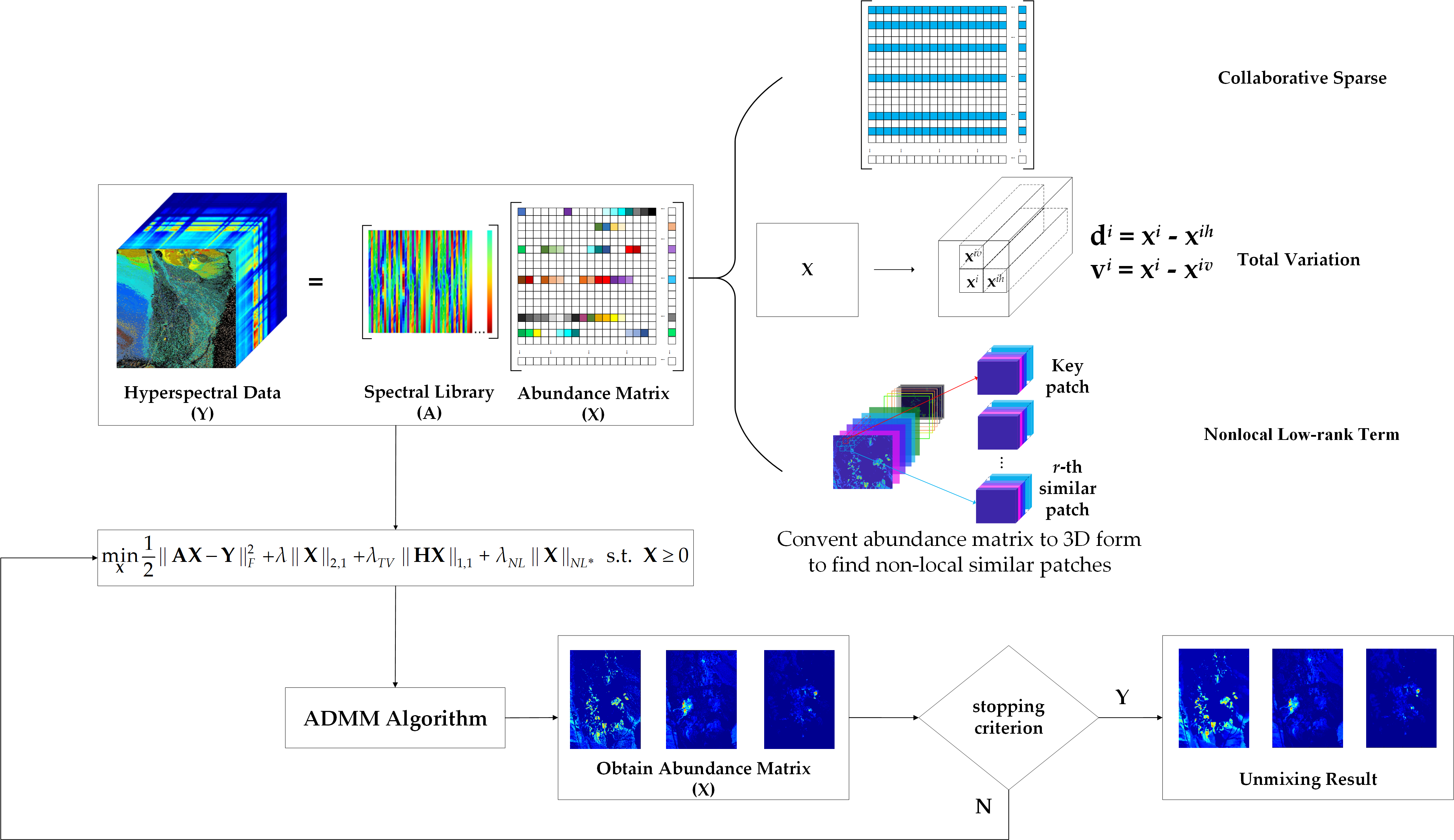
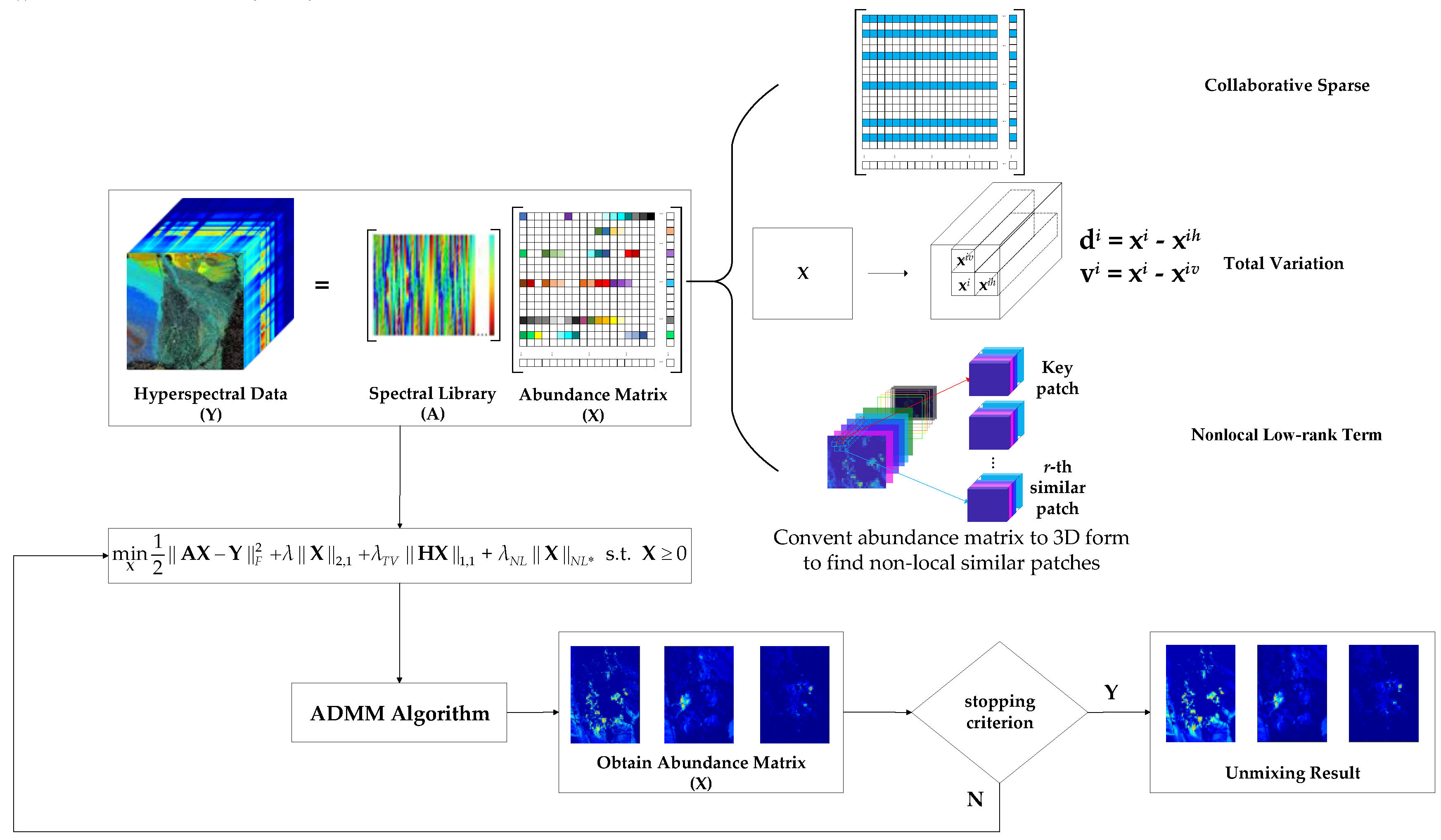
The non-local low-rank regularization can help to preserve the details of the image better than the state-of-the-art algorithms. In addition, the proposed algorithm utilizes both spectral and spatial information simultaneously to obtain better unmixing results.

(2)

In order to improve unmixing performance, a large spectral library is used as an endmember matrix instead of extracting endmembers from the hyperspectral image directly.

(3)

The optimization problem of the proposed algorithm with all convex terms is solved by the alternating direction multiplier method (ADMM).

(4)

Extensive experiments on both simulated and real data sets validate the superiority of the proposed method in unmixing hyperspectral images.

The rest of this paper is organized as follows. In Section 2, we discuss the linear spectral unmixing and sparse unmixing problem. In Section 3, we describe the proposed NLLRSU algorithm and optimization. In Section 4, we test the proposed algorithm and other sparse unmixing algorithms with two simulated data sets and two real hyperspectral data sets. Finally, we summarize this paper in Section 5.

2. Related Works

2.1. Linear Spectral Unmixing

The linear mixed model (LMM) assumes that each pixel spectrum can be linearly combined by all endmembers and corresponding abundances exist in the pixel [57]. The linear model can be described as follows:

$$y={\displaystyle \sum _{i=1}^q{m}_i{\alpha }_i+n}=M\alpha +n,$$

(1)

where $y\in {ℝ}^{l\times 1}$ is a column vector which represents a mixed pixel and l is the number of bands, $M\in {ℝ}^{l\times q}$ is an endmember matrix and q is the number of endmembers, $\alpha \in {ℝ}^{q\times 1}$ represents the abundance vector of the endmembers, $n\in {ℝ}^{l\times 1}$ is the model error and noise that are generated during the observation process.

To ensure that the solution of the abundance has the physical meaning, the LMM introduces two constraints, named the abundance non-negativity constraint (ANC) and the abundance sum-to-one constraint (ASC) [58], which are expressed as:

$$\mathrm{ANC}:{\alpha }_i\ge 0\hspace{1em}(i=1,2,\dots ,q),$$

(2)

$$\mathrm{ASC}:{\displaystyle \sum _{i=1}^q{\alpha }_i=1}$$

(3)

In a hyperspectral scene, let $Y\in {ℝ}^{l\times s}$ be the observed hyperspectral image data and $X\in {ℝ}^{q\times s}$ be the abundance matrix, where s is the number of pixels in the hyperspectral image. Equation (1) can be rewritten as:

$$Y=MX+N,$$

(4)

where ${\rm N}\in {ℝ}^{l\times s}$ represents noise and model error.

2.2. Sparse Unmixing

The sparse unmixing utilizes a large spectral library $A\in {ℝ}^{l\times t}$ instead of the endmember matrix, where t is the number of spectral signatures of ground material in the spectral library A. The model can be described as:

$$Y=AX+N,$$

(5)

where $X\in {ℝ}^{t\times s}$ is the abundance matrix corresponding to the spectral library A.

The number of spectral characteristics in the spectral library A is usually far more than the number of endmembers in a given real hyperspectral scene. Thus, the abundance matrix X contains many zero values, so the abundance matrix is considered as sparse. Therefore, the sparse unmixing model can be expressed as:

$$\underset{X}{\min }\frac{1}{2}||AX-Y|{|}_F^2+\lambda ||X|{|}_0\hspace{1em}\mathrm{s}.\mathrm{t}.\hspace{1em}X\ge 0,$$

(6)

where $||AX-Y|{|}_F^2$ represents the reconstruction error of the model and $||X|{|}_F\equiv \sqrt{\mathrm{trace}\left\{X{X}^T\right\}}$ is the Frobenius norm of the X, $||X|{|}_0$ is the L₀ norm of the abundance matrix X, which denotes the number of non-zero elements in X. Here, we do not introduce the ASC constraint to Equation (6) because ASC has received extensive criticism from scholars [31].

Since the L₀ norm is non-convex, the problem of minimization of Equation (6) is difficult to solve. Recently, one theory proved that when the spectral library matrix A satisfies the restricted isometry property (RIP) condition [59], the L₀ norm problem can be equivalently converted to the L₁ norm problem, which is a convex optimization problem and easier to solve. Therefore, we can replace the L₀ norm by the L₁ norm to transform the nonconvex optimization problem into a convex one. Accordingly, Equation (6) can be rewritten as:

$$\underset{X}{\min }\frac{1}{2}||AX-Y|{|}_F^2+\lambda ||X|{|}_1\hspace{1em}\mathrm{s}.\mathrm{t}.\hspace{1em}X\ge 0,$$

(7)

where $||X|{|}_1\equiv {\displaystyle {\sum }_{i=1}^t{\displaystyle {\sum }_{j=1}^s|{\mathrm{x}}_{ij}|}}$ is the L₁ norm which calculates the sum of the elements in the abundance matrix X.

In practice, one hyperspectral scene often has only a few endmembers out of a large spectral library. CLSUnSAL algorithm enforces the column (pixels) of the abundance matrix X share the same active set of endmembers, so X has only a few nonzero rows (endmembers). That is, X has the characteristics of sparse among the rows. To utilize this prior, CLSUnSAL replaces the L₁ norm by L_2,1 norm which is sparser than the L₁ norm. The equation of CLSUnSAL algorithm is expressed as follows:

$$\underset{X}{\min }\frac{1}{2}||AX-Y|{|}_F^2+\lambda ||X|{|}_{2,1}\hspace{1em}\hspace{1em}\mathrm{s}.\mathrm{t}.\hspace{1em}\hspace{1em}X\ge 0,$$

(8)

where $||X|{|}_{2,1}\equiv {\displaystyle {\sum }_{i=1}^t||x_i|{|}_2}\equiv {\displaystyle {\sum }_{i=1}^t\sqrt{{\displaystyle {\sum }_{j=1}^s|{\mathrm{x}}_{ij}{|}^2}}}$ is the L_2,1 norm of the abundance matrix X and $x_i$ represents the i-th row of X.

In addition to utilizing the properties of the spectrum, the spatial correlation of hyperspectral images is also beneficial for improving the result of the unmixing. Each pixel and its neighboring pixels usually contain similar material, so the spectral characteristic between these pixels are very similar. To promote smoothness between adjacent pixels, the TV regularization term, which describes spatial correlation, can be applied to Equation (7). Then, the model is:

$$\underset{X}{\min }\frac{1}{2}||AX-Y|{|}_F^2+\lambda ||X|{|}_1+{\lambda }_{TV}\mathrm{TV}(X)\hspace{1em}\mathrm{s}.\mathrm{t}.\hspace{1em}X\ge 0,$$

(9)

where

$$\mathrm{TV}(X)\equiv {\displaystyle \sum _{\{i,j\}\in \epsilon }||x^i-x^j|{|}_1},$$

(10)

represent nonisotropic TV, $x^i$ and $x^j$ are i-th and j-th columns of X, respectively, $\epsilon$ denotes the set that contains horizontal and vertical neighbors in a hyperspectral image [42].

Let $H_h:{ℝ}^{t\times s}\to {ℝ}^{t\times s}$ and $H_v:{ℝ}^{t\times s}\to {ℝ}^{t\times s}$ represent the horizontal and vertical differential linear operators of adjacent pixels in the abundance matrix X, respectively. $H_{h}X=[d^1,d^2,\dots ,d^s]$ calculates the difference of the X and horizontal neighboring pixels, where $d^i=x^i-x^{ih}$, $x^i$ is a column vector and $x^{ih}$ is the horizontal neighboring column vector of $x^i$. Similar to $H_{h}X$, $H_{v}X=[v^1,v^2,\dots ,v^s]$ calculates the vertical difference, where $v^i=x^i-x^{iv}$, $x^i$ is a column vector and $x^{iv}$ is the vertical neighboring column vector of $x^i$. By horizontal and vertical operations, we can obtain $HX\equiv \left[H_{h}X;H_{v}X\right]$ [42,60]. Therefore, Equation (9) can be rewritten as:

$$\underset{X}{\min }\frac{1}{2}||AX-Y|{|}_F^2+\lambda ||X|{|}_1+{\lambda }_{TV}||HX|{|}_1\hspace{1em}\mathrm{s}.\mathrm{t}.\hspace{1em}X\ge 0,$$

(11)

However, CLSUnSAL only considers the sparsity of the abundance from a perspective in the spectral domain. SUnSAL-TV only exploits the local smoothness in the spectral domain, it may cause over smoothing in the edge regions. There is still much room for improving the unmixing performance. Therefore, we propose a nonlocal low-rank prior to the sparse unmixing (NLLRSU) algorithm to obtain more precise spatial information by exploiting the nonlocal self-similarity.

3. Proposed Algorithm

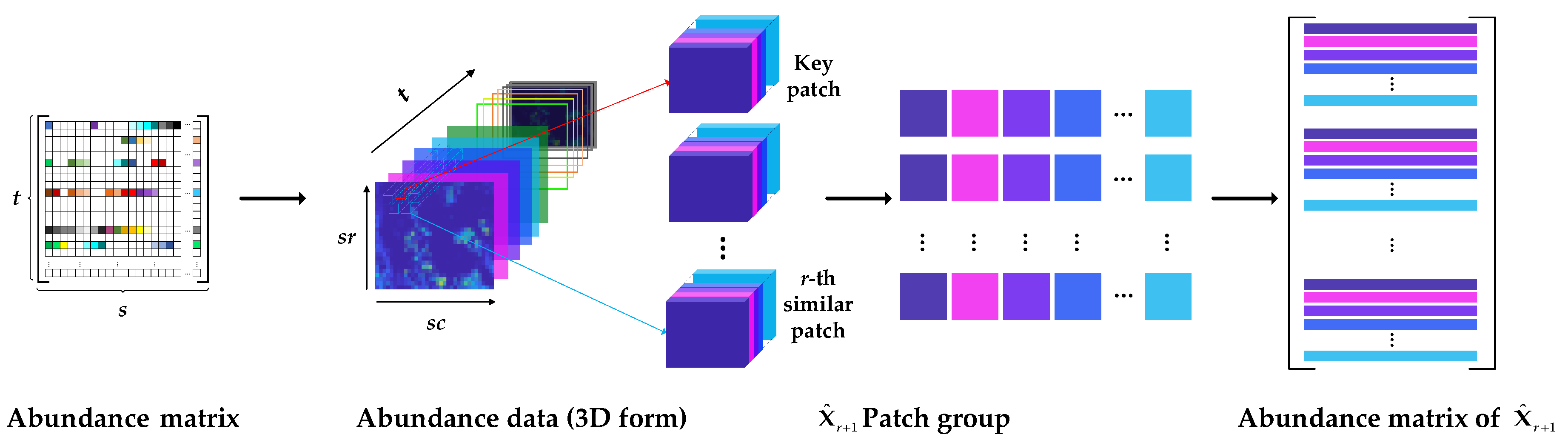
3.1. Nonlocal Self-Similarity

Treated as a natural image in each band, hyperspectral images are smooth in local regions between adjacent pixels and bands, meanwhile, they are self-similar in nonlocal regions. The adjacent pixels have smooth property. Therefore, there is a high correlation between the pixels of the local regions in the hyperspectral images, that is, the pixels are very likely to contain the same material in a local region. In addition, there are a large number of similar structural information in different regions in the hyperspectral images. These similar structures consist of smooth regions, texture regions, and edge regions. For any local region, we can find many similar regions in the image. That is to say, the information of the hyperspectral image itself is redundant and the pixels in these similar regions are also very likely to contain the same material. Qu et al. [44] indicated that this high spatial correlation of hyperspectral images means that there is also a high correlation in the abundance matrix, which is reflected by the linear correlation between the abundance vectors. Based on this prior, the abundance matrix can be reconstructed by the proposed nonlocal low-rank algorithm.

In order to take advantage of the nonlocal low-rank property, we need to search for similar structural texture regions in the abundance matrix. Therefore, we convert the abundance matrix to 3D abundance cube, which restores the position of the pixels and spectral bands in the abundance matrix to the corresponding position in the original 3D abundance cube, then we use a small 3D sliding patch on this abundance cube. For each small 3D patch, denoted by a key patch, we can find several small patches similar to this key patch in the abundance cube by utilizing a block matching algorithm [56]. Then, we stack the key patch and these similar patches to generate a patch group and use the nuclear norm to enforce the low-rank property to this patch group. To sum up, the small 3D patch slides across all dimensions of the abundance cube and the proposed nonlocal low-rank regularization term employs the nuclear norm to enforce the low-rank property of each patch group.

In addition, the results of sparse unmixing are affected by the correlation between spectral characteristics in the spectral library [61]. In general, a spectral library contains many spectral characteristics of the same ground materials in different situations. The similarity between these spectral signatures is very high, which leads to the conclusion that the solution of the sparse unmixed model is not unique. To overcome this disadvantage, we need to ensure that the linear correlation between the spectral characteristics in the spectral library is as small as possible. Therefore, we use a strategy to precondition the spectral library. Given a spectral library A, we calculate the spectral angle ${\theta }_{i,j}$ between any two different spectral characteristics $A_i$ and $A_j$. The ${\theta }_{i,j}$ is defined as follows:

$${\theta }_{i,j}={\cos }^{-1}\left(\frac{A_i^T{A}_j}{|A_i||A_j|}\right),$$

(12)

Any two spectral characteristics in spectral library A are regarded as linear correlation if the spectral angle ${\theta }_{i,j}$ of the two spectral characteristics is less than a given threshold. We reserve one of these linear correlation spectral characteristics and discard the remaining linear correlation spectral characteristics. With this operation, we obtain a pruned spectral library which is utilized for sparse unmixing.

3.2. Nonlocal Low-Rank Regularization

In the former section, we explained how the abundance matrix is converted to 3D form to find similar structural information. Let $\widehat{X}\in {ℝ}^{sr\times sc\times t}$ be the 3D form of the abundance data, where sr and sc represent the number of rows and columns, respectively, and $s=sr\times sc$ is the number of pixels in the abundance matrix and t is the number of signatures in the spectral library. Assuming that the number of patches is P in $\widehat{X}$ and ${\widehat{X}}_p\in {ℝ}^{sp\times sp\times tp}$ is the p-th patch, where $p=1,2,\dots ,P$. Taking the p-th patch as an example, we use a block matching algorithm [56] to find the r nonlocal patches which are similar to the p-th patch. Then, with the r+1 patches together, we generate a patch group, which is denoted by ${\widehat{X}}_{r+1}\in {ℝ}^{sp\times sp\times u}$ and $u=tp\times (r+1)$. For each spectral dimension in the patch group, denoted by ${\widehat{X}}_{i,r+1}\in {ℝ}^{sp\times sp}$, where $i=1,2,\dots ,u$, we convert it to a vector, denoted by ${\widehat{x}}_{i,r+1}\in {ℝ}^w$, where $w=sp\times sp$. Figure 2 illustrates this process. Finally, we obtain the abundance matrix of the patch group by:

$$D_{{\widehat{X}}_{r+1}}=({\widehat{x}}_{1,r+1},{\widehat{x}}_{2,r+1},\dots ,{\widehat{x}}_{u,r+1})\in {ℝ}^{u\times w}$$

(13)

The nuclear norm is then imposed to enforce the low-rank property of the abundance map $D_{{\widehat{X}}_{r+1}}$ of the patch group ${\widehat{X}}_{r+1}$:

$$||D_{{\widehat{X}}_{r+1}}|{|}_{*}={\displaystyle \sum _{j=1}^{rank(D_{{\widehat{X}}_{r+1}})}{\sigma }_j(D_{{\widehat{X}}_{r+1}})},$$

(14)

where ${\sigma }_j$ represents the j-th singular value, where $j=1,2,\dots ,rank(D_{{\widehat{X}}_{r+1}})$. Therefore, the estimated abundance matrix of this patch group can be enforced by the low-rank constraint. At last, we aggregate the estimated abundance matrix to the corresponding position of each patch in the patch group. Similarly, we conduct this operation for all P number of patches. For the whole abundance matrix X, we use $||X|{|}_{NL*}$ to represent the nonlocal low-rank regularization term.

3.3. Proposed Model and Optimization

Based on the sparse unmixing model, the proposed NLLRSU algorithm has three regularizers, named collaborative sparsity, TV, and nonlocal abundance low-rankness. The model is formulated as follows:

$$\underset{X}{\min }\frac{1}{2}||AX-Y|{|}_F^2+\lambda ||X|{|}_{2,1}+{\lambda }_{TV}||HX|{|}_1+{\lambda }_{NL}||X|{|}_{NL*}+l_{R+}(X),$$

(15)

where $\lambda ,{\lambda }_{TV},{\lambda }_{NL}$ are the parameters of the collaborative sparsity, TV, and nonlocal low-rank regularization terms, respectively. $l_{R+}(x)$ is an indicator function, when $x\ge 0$, $l_{R+}(x)=0$; otherwise $l_{R+}(X)=+\infty$, it is utilized to ensure ANC constraint.

It is difficult to optimize the model (15) directly, so we employ the ADMM [37] to solve it. The core idea of ADMM is that a difficult problem can be transformed into several simple subproblems by introducing some new variables cautiously. The subproblems are solved one by one and alternately updated. Here, we introduce the variables $V_1,V_2,V_3,V_4,V_5,V_6$. Then the Equation (15) can be rewritten as:

$$\begin{array}{c}\underset{X,V_1,V_2,V_3,V_4,V_5,V_6}{\min }\frac{1}{2}||V_1-Y|{|}_F^2+\lambda ||V_2|{|}_{2,1}+{\lambda }_{TV}||V_4|{|}_1+{\lambda }_{NL}||V_5|{|}_{NL*}+l_{R+}(V_6)\\ \mathrm{s}.\mathrm{t}.V_1=AX\\ V_2=X\\ V_3=X\\ V_4=H{V}_3\\ V_5=X\\ V_6=X\end{array}$$

(16)

The Lagrangian function of the Equation (16) is:

$$\begin{array}{c}ℒ(X,V_1,V_2,V_3,V_4,V_5,V_6,D_1,D_2,D_3,D_4,D_5,D_6)\\ =\frac{1}{2}||V_1-Y|{|}_F^2+\lambda ||V_2|{|}_{2,1}+{\lambda }_{TV}||V_4|{|}_1+{\lambda }_{NL}||V_5|{|}_{NL*}\\ +l_{R+}(V_6)+\frac{\mu }{2}||V_1-AX+D_1|{|}_F^2+\frac{\mu }{2}||V_2-X+D_2|{|}_F^2\\ +\frac{\mu }{2}||V_3-X+D_3|{|}_F^2+\frac{\mu }{2}||V_4-H{V}_3+D_4|{|}_F^2\\ +\frac{\mu }{2}||V_5-X+D_5|{|}_F^2+\frac{\mu }{2}||V_6-X+D_6|{|}_F^2\end{array}$$

(17)

where $D_1,D_2,D_3,D_4,D_5,D_6$ are Lagrangian multipliers and $\mu$ is the Lagrangian parameter.

Algorithm 1 gives the pseudocode for the NLLRSU solution process. In each iteration, with the ADMM, we optimize $X,V_1,V_2,V_3,V_4,V_5,V_6$ in sequence, then we update the Lagrangian multipliers $D_1,D_2,D_3,D_4,D_5,D_6$.

Next, we discuss the details of step 3 in Algorithm 1, which is utilized to compute the value of variable X at each iteration. In this step, we fix other variables and update X only. The optimization problem for step 3 can be written as:

$$\begin{array}{c}{X}^{(k+1)}\leftarrow \underset{X}{\mathrm{argmin}}\frac{\mu }{2}||V_1^{(k)}-AX+D_1^{(k)}|{|}_F^2+\frac{\mu }{2}||V_2^{(k)}-X+D_2^{(k)}|{|}_F^2\\ +\frac{\mu }{2}||V_3^{(k)}-X+D_3^{(k)}|{|}_F^2+\frac{\mu }{2}||V_5^{(k)}-X+D_5^{(k)}|{|}_F^2+\frac{\mu }{2}||V_6^{(k)}-X+D_6^{(k)}|{|}_F^2\end{array}$$

(18)

The solution of Equation (18) is:

$$X^{(k+1)}\leftarrow {(A^{T}A+4I)}^{-1}(A^T{\xi }_1+{\xi }_2+{\xi }_3+{\xi }_5+{\xi }_6)$$

(19)

where A^T is the transpose of A, I is the identity matrix, and ${\xi }_1=V_1^{(k)}+D_1^{(k)}$,${\xi }_2=V_2^{(k)}+D_2^{(k)}$, ${\xi }_3=V_3^{(k)}+D_3^{(k)}$, ${\xi }_5=V_5^{(k)}+D_5^{(k)}$, ${\xi }_6=V_6^{(k)}+D_6^{(k)}$.

Algorithm 1: Pseudocode of the NLLRSU algorithm.

Initialization: set $k=0$, choose $\mu ,\lambda ,{\lambda }_{TV},{\lambda }_{NL},X^{(0)},V_1^{(0)},\dots ,V_6^{(0)},D_1^{(0)},\dots ,D_6^{(0)}$ while some stopping criterion is not satisfied do $X^{(k+1)}\leftarrow \underset{X}{\mathrm{argmin}}ℒ(X,V_1^{(k)},\dots ,V_6^{(k)},D_1^{(k)},\dots ,D_6^{(k)})$ for i = 1,…,6 do $V_i^{(k+1)}\leftarrow \underset{V_i}{\mathrm{argmin}}ℒ(X^{(k)},V_1^{(k)},\dots ,V_i,\dots ,V_6^{(k)})$ end for Update Lagrange multipliers $D_1^{(k+1)}\leftarrow D_1^{(k)}-A{X}^{(k+1)}+V_1^{(k+1)}$ $D_4^{(k+1)}\leftarrow D_4^{(k)}-H{V}_3^{(k+1)}+V_4^{(k+1)}$ $D_i^{(k+1)}\leftarrow D_i^{(k)}-X^{(k+1)}+V_i^{(k+1)},i=2,3,5,6$ Update iteration $k=k+1$ end while

Now, we introduce solutions of the variables V₁, V₂, V₃, V₄, V₅, V₆ in step 5 of Algorithm 1. To solve V₁, the optimization problem for V₁ can be described as:

$$V_1^{(k+1)}\leftarrow \underset{V_1}{\mathrm{argmin}}\frac{1}{2}||V_1-Y|{|}_F^2+\frac{\mu }{2}||V_1-A{X}^{(k)}+D_1^{(k)}|{|}_F^2$$

(20)

The solution of V₁ is:

$$V_1^{(k+1)}\leftarrow \frac{1}{1+\mu }[Y+\mu (A{X}^{(k)}-D_1^{(k)})]$$

(21)

The optimization problem of V₂ is:

$$V_2^{(k+1)}\leftarrow \underset{V_2}{\mathrm{argmin}}\lambda ||V_2|{|}_{2,1}+\frac{\mu }{2}||V_2-X^{(k)}+D_2^{(k)}|{|}_F^2$$

(22)

The solution of V₂ is given by using the famous vect-soft threshold [62]:

$$V_2^{(k+1)}\leftarrow \mathrm{vect}\text{-}\mathrm{soft}(X^{(k)}-D_2^{(k)},\frac{\lambda }{\mu })$$

(23)

where $\mathrm{vect}\text{-}\mathrm{soft}(\cdot ,\psi )$ means that the vect-soft threshold function is applied row by row, and the vect-soft threshold function is $x\mapsto x(\max \{||x|{|}_2-\psi ,0\}/\max \{||x|{|}_2-\psi ,0\}+\psi )$, $\psi$ is a threshold.

To compute V₃, we need to solve the following problem:

$$V_3^{(k+1)}\leftarrow \underset{V_3}{\mathrm{argmin}}\frac{\mu }{2}||V_3-X^{(k)}+D_3^{(k)}|{|}_F^2+\frac{\mu }{2}||V_4^{(k)}-H{V}_3+D_4^{(k)}|{|}_F^2$$

(24)

The solution of V₃ is:

$$V_3^{(k+1)}\leftarrow {(H^{T}H+I)}^{-1}(X^{(k)}-D_3^{(k)}+H^T(V_4^{(k)}+D_4^{(k)}))$$

(25)

where H represents a convolution. H can be applied independently in a band-by-band manner and calculated by discrete Fourier transform diagonalization [63].

The optimization problem of V₄ is:

$$V_4^{(k+1)}\leftarrow \underset{V_4}{\mathrm{argmin}}{\lambda }_{TV}||V_4|{|}_1+\frac{\mu }{2}||V_4-H{V}_3^{(k)}+D_4^{(k)}|{|}_F^2$$

(26)

The solution of V₄ can be obtained by soft-threshold [64]:

$$V_4^{(k+1)}\leftarrow \mathrm{soft}(D_4^{(k)}-H{V}_3^{(k)},\frac{{\lambda }_{TV}}{\mu })$$

(27)

where $\mathrm{soft}(\cdot ,\psi )$ represents the soft-threshold function $x\mapsto \mathrm{sign}(x)\max \{|x|-\psi ,0\}$.

To obtain the solution of V₅, the optimization problem of (28) should be solved.

$$V_5^{(k+1)}\leftarrow \underset{V_5}{\mathrm{argmin}}{\lambda }_{NL}||V_5|{|}_{NL*}+\frac{\mu }{2}||V_5-X^{(k)}+D_5^{(k)}|{|}_F^2$$

(28)

For the abundance matrix $D_{{\widehat{X}}_{r+1}}$ of each patch group, we apply singular value shrinkage to obtain the reconstructed abundance matrix. The solution of V₅ can be expressed as:

$$V_5^{(k+1)}\leftarrow \mathrm{shrinkage}(X^{(k)}-D_5^{(k)},\frac{{\lambda }_{NL}}{\mu })$$

(29)

where $\mathrm{shrinkage}(\cdot ,\psi )$ is the singular value shrinkage $x\mapsto \mathrm{diag}(\max \{SVD\left(x\right)-\psi ,0\left\}\right)$ of abundance matrix $D_{{\widehat{X}}_{r+1}}$.

Finally, the optimization problem of V₆ is as follows:

$$V_6^{(k+1)}\leftarrow \underset{V_6}{\mathrm{argmin}}{l}_{R+}(V_6)+\frac{\mu }{2}||V_6-X^{(k)}+D_6^{(k)}|{|}_F^2$$

(30)

The solution of V₆ is:

$$V_6^{(k+1)}\leftarrow \max (X^{\left(k\right)}-D_6^{(k)},0)$$

(31)

3.4. Computational Complexity

In this algorithm, the most time-consuming procedures are calculating X, V₃, and V₅, and the corresponding complexities are O(l²s), O(lslogs), and O(wu²P), respectively, where s is the total number of pixels in a hyperspectral image, l is the number of spectral characteristics, w and u are the number of pixels and bands in one patch group, respectively, and P is the number of patches. In each iteration, V₅, the singular value decomposition step, costs the most time. Thus, the overall complexity of this algorithm is O(wu²P).

4. Experiment and Analysis

In order to test the unmixing performance of the proposed algorithm, we used two simulated data sets and two real hyperspectral image data sets. For each simulated data set, our experiments were performed in three different signal-to-noise ratio (SNR) levels, 10dB, 15dB, and 20dB. We also compared the proposed algorithm with SUnSAL [31], CLSUnSAL [38], SUnSAL-TV [42], J-LASU [55], and L₁-L₂ SUnSAL-TV [43].

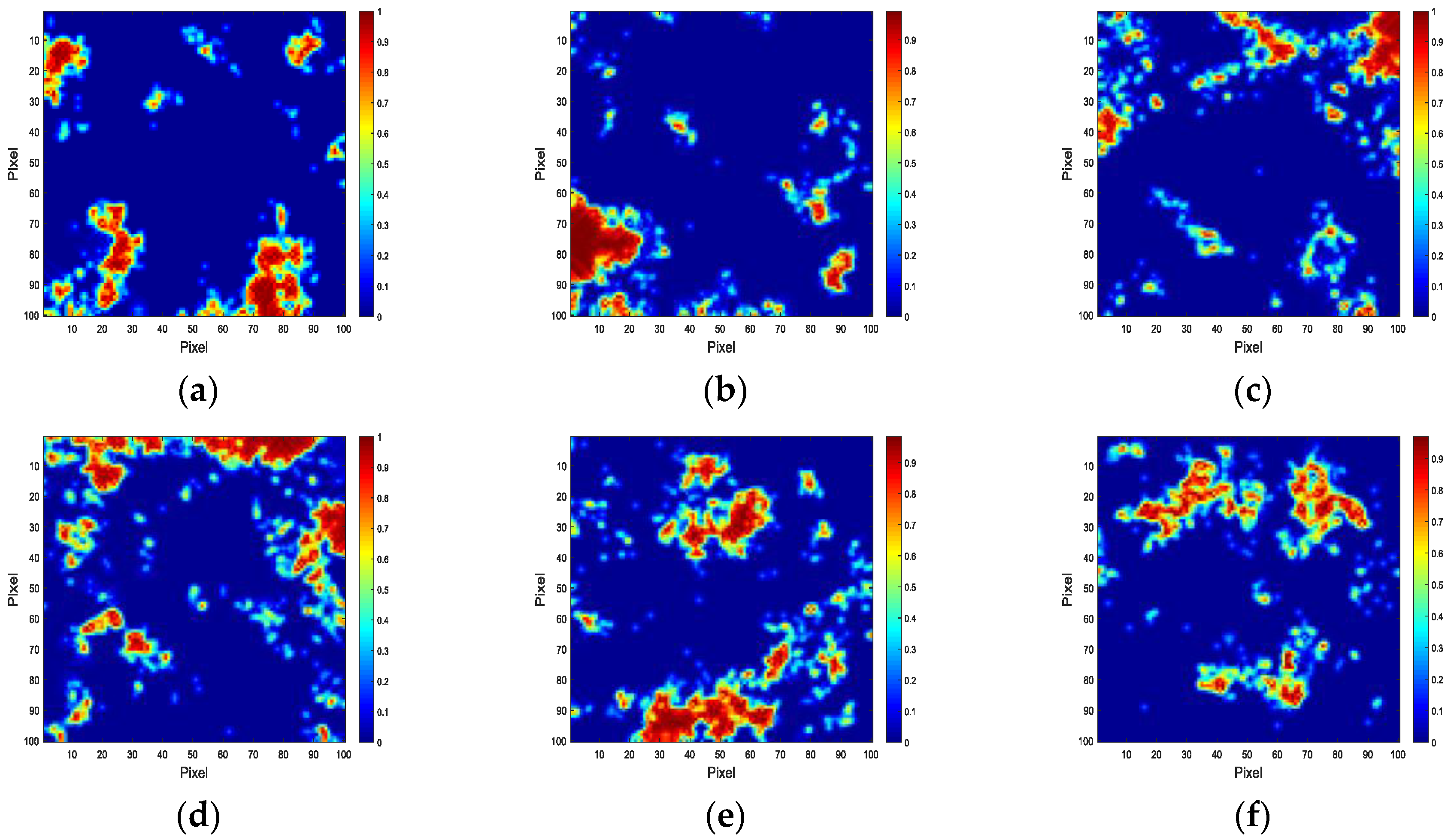
4.1. Experiments with Simulated Data

In this paper, we employed splib06 [65], a USGS spectral library released in September 2007, to our experiments. We selected 240 endmember signatures randomly from the splib06 as the spectral library, denoted by $A\in {ℝ}^{224\times 240}$, and the spectral library A contains 224 bands of spectra with spectral range from 0.4 to 2.5 μm. Because the linear correlation between the spectral characteristics is very high, we set the spectral angle to be larger than 4.4 to avoid this problem.

The simulated data set 1 (DS1) was generated by randomly selecting five spectral characteristics from the spectral library A and following the linear mixed model. DS1 has $75\times 75$ pixels and each pixel has 224 bands and the corresponding abundance is constrained by ASC. Figure 3a illustrated the composition of the DS1. In DS1, some square regions are pure and some regions are mixed by two to five endmembers. The background pixels of this data set are composed of the same five endmembers with randomly fixed abundance values 0.1149, 0.0741, 0.2003, 0.2055, and 0.4051. Figure 3b–f shows the true abundances of five endmembers. After generating DS1, we applied three different SNR levels Gaussian noise, 10dB, 15dB, and 20dB, to this data set.

The simulated data set 2 (DS2) contains nine spectral characteristics which are randomly selected from spectral library A and has $100\times 100$ pixels. The abundances of nine spectral signatures obey a Dirichlet distribution uniformly over the probability simplex and are constrained by ANC and ASC. As shown in Figure 4, the abundances of DS2 shows the piecewise smoothness in the spatial domain and their distributions are closer to those of the real data sets. After generating DS2, this data set is distorted by Gaussian noise with the same SNR levels as DS1.

In the simulated data experiment, the parameters $\lambda$ represent sparsity term for SUnSAL, CLSUnSAL, SUnSAL-TV, J-LASU, L₁-L₂ SUnSAL-TV, and NLLRSU. The TV term for SUnSAL-TV, J-LASU, L₁-L₂ SUnSAL-TV, and NLLRSU is represented by ${\lambda }_{TV}$. For J-LASU, the local low-rank term is controlled by ${\lambda }_{LR}$ and the local block size is set to $5\times 5\times 5$ with no overlap according to J-LASU. The ${\lambda }_{NL}$ means nonlocal abundance low-rank term for NLLRSU and each local patch size is set to $5\times 5\times 5$ and we find the four patches which are similar to the local patch after several experiments. The parameters $\lambda$, ${\lambda }_{TV}$, ${\lambda }_{LR}$, ${\lambda }_{NL}$ are selected between 10^-4 to 10. For each algorithm, we adjust each parameter to the optimal value.

Table 1. Parameter settings.

Data		DS1			DS2
SNR		10dB	15dB	20dB	10dB	15dB	20dB
SUnSAL [31]	$\lambda$	$1\times {10}^0$	$5\times {10}^{-1}$	$1\times {10}^{-1}$	$5\times {10}^{-1}$	$1\times {10}^{-1}$	$1\times {10}^{-1}$
CLSUnSAL [38]	$\lambda$	$1\times {10}^1$	$1\times {10}^1$	$8\times {10}^0$	$1\times {10}^1$	$1\times {10}^1$	$3\times {10}^0$
SUnSAL-TV [42]	$\lambda$	$1\times {10}^{-1}$	$1\times {10}^{-1}$	$5\times {10}^{-2}$	$1\times {10}^{-1}$	$1\times {10}^{-1}$	$5\times {10}^{-2}$
	${\lambda }_{TV}$	$5\times {10}^{-1}$	$1\times {10}^{-1}$	$5\times {10}^{-2}$	$1\times {10}^{-1}$	$5\times {10}^{-2}$	$1\times {10}^{-2}$
J-LASU [55]	$\lambda$	$2\times {10}^0$	$1\times {10}^0$	$2.5\times {10}^{-1}$	$1\times {10}^{-4}$	$1\times {10}^{-4}$	$1\times {10}^{-4}$
	${\lambda }_{TV}$	$1\times {10}^{-1}$	$1\times {10}^{-1}$	$5\times {10}^{-2}$	$5\times {10}^{-2}$	$5\times {10}^{-2}$	$1\times {10}^{-2}$
	${\lambda }_{LR}$	$1\times {10}^0$	$5\times {10}^{-1}$	$3\times {10}^{-1}$	$5\times {10}^{-1}$	$1\times {10}^{-1}$	$1\times {10}^{-1}$
L1-L2 SUnSAL-TV [43]	$\lambda$	$1\times {10}^{-2}$	$1\times {10}^{-1}$	$1\times {10}^{-2}$	$1\times {10}^{-1}$	$1\times {10}^{-2}$	$1\times {10}^{-2}$
	${\lambda }_{TV}$	$5\times {10}^{-1}$	$5\times {10}^{-2}$	$5\times {10}^{-2}$	$1\times {10}^{-1}$	$5\times {10}^{-2}$	$5\times {10}^{-2}$
NLLRSU	$\lambda$	$5\times {10}^{-1}$	$1\times {10}^{-1}$	$1\times {10}^{-1}$	$1\times {10}^{-4}$	$1\times {10}^{-4}$	$1\times {10}^{-4}$
	${\lambda }_{TV}$	$1\times {10}^{-1}$	$1\times {10}^{-1}$	$5\times {10}^{-2}$	$1\times {10}^{-1}$	$5\times {10}^{-2}$	$1\times {10}^{-2}$
	${\lambda }_{NL}$	$2\times {10}^0$	$5\times {10}^{-1}$	$5\times {10}^{-1}$	$1\times {10}^0$	$5\times {10}^{-1}$	$1\times {10}^{-1}$

shows these parameter settings.

We employ two evaluation indicators to assess the quality of the six algorithms: signal reconstruction error (SRE) [66] and root mean square error (RMSE) [67]. SRE is the ratio between the reconstructed abundance matrix and error, and higher SRE value indicates a better result. SRE can be defined as follows:

$$\mathrm{SRE}\left(\mathrm{dB}\right)=10{\log }_{10}\frac{\mathrm{E}[||X|{|}_2^2]}{\mathrm{E}[||X-\widehat{X}|{|}_2^2]},$$

(32)

where X is the true abundance matrix and $\widehat{X}$ is the estimated abundance matrix.

RMSE represents the error between the true abundance matrix and the estimated abundance matrix, and lower RMSE value indicates more accurate estimation of abundance matrix. RMSE can be defined as follows:

$$\mathrm{RMSE}=\sqrt{\frac{1}{t\times s}{\displaystyle \sum _{i=1}^t{\displaystyle \sum _{j=1}^s{(x_{ij}-{\widehat{x}}_{ij})}^2}}},$$

(33)

where $x_{ij}$ and ${\widehat{x}}_{ij}$ represent each element in the true abundance matrix and the estimated abundance matrix, respectively.

Figure 5 shows SRE(dB) values of NLLRSU as a function of parameters $\lambda$, ${\lambda }_{TV}$, and ${\lambda }_{NL}$ in 20dB SNR level. Since there are three parameters, we considering the effect of ($\lambda$ and ${\lambda }_{TV}$), ($\lambda$ and ${\lambda }_{NL}$), (${\lambda }_{TV}$ and ${\lambda }_{NL}$) on SRE value, respectively, while the other parameters are set to the optimal values. From Figure 5, we can observe that relatively smaller parameter values result in better SRE values.

Figure 6, Figure 7, Figure 8 and Figure 9 show the abundance image reconstructed by the six algorithms for one randomly selected endmember in DS1 and DS2 with 20db SNR level, respectively. From 8 and 9, we can clearly see that SUnSAL-TV algorithm shows the smoothest results in the edge regions. Nevertheless, the edge transition regions reconstructed by our algorithm is closer to the true abundance distribution. The result shows that nonlocal low-rank regularization terms keep the structure information of the image better than other algorithms.

Table 2. SRE (dB) result (The optimal results are shown in bold type).

Data	SNR	SUnSAL [31]	CLSUnSAL [38]	SUnSAL-TV [42]	J-LASU [55]	L1-L2 SUnSAL-TV [43]	NLLRSU
DS1	10dB	0.2017	1.6544	3.9803	10.6039	4.1424	11.5466
	15dB	0.9448	4.4945	6.4204	13.4001	6.0267	13.9307
	20dB	2.4218	6.0518	7.1069	15.3860	7.0245	16.2008
DS2	10dB	1.2568	1.0144	3.6093	3.5925	3.6494	3.9300
	15dB	1.9727	2.3747	4.5860	4.8039	4.8445	5.1034
	20dB	4.1627	3.3961	5.5352	6.3062	6.2078	6.7188

and

Table 3. Root mean square error (RMSE) result (The optimal results are shown in bold type).

Data	SNR	SUnSAL [31]	CLSUnSAL [38]	SUnSAL-TV [42]	J-LASU [55]	L1-L2 SUnSAL-TV [43]	NLLRSU
DS1	10dB	0.0338	0.0286	0.0218	0.0102	0.0214	0.0091
	15dB	0.0310	0.0206	0.0165	0.0074	0.0173	0.0069
	20dB	0.0261	0.0172	0.0152	0.0059	0.0154	0.0054
DS2	10dB	0.0426	0.0438	0.0325	0.0325	0.0323	0.0313
	15dB	0.0392	0.0374	0.0290	0.0283	0.0282	0.0273
	20dB	0.0305	0.0333	0.0260	0.0238	0.0241	0.0227

show the values of SRE (dB) and RMSE of the six algorithms with two simulated data sets, respectively. From these tables, we can observe that the performance of the proposed NLLRSU algorithm is better than other state-of-the-art algorithms in the same SNR level.

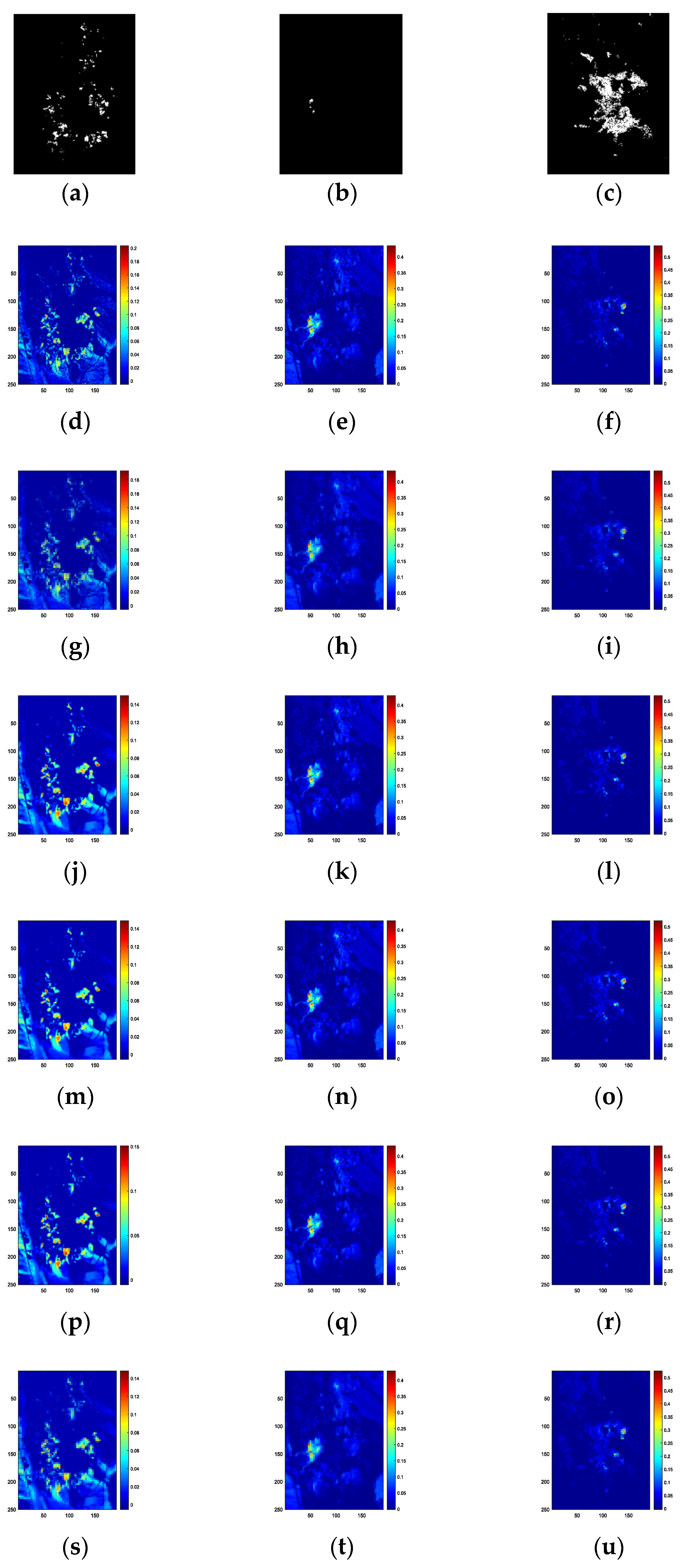
4.2. Experiments with Real Data

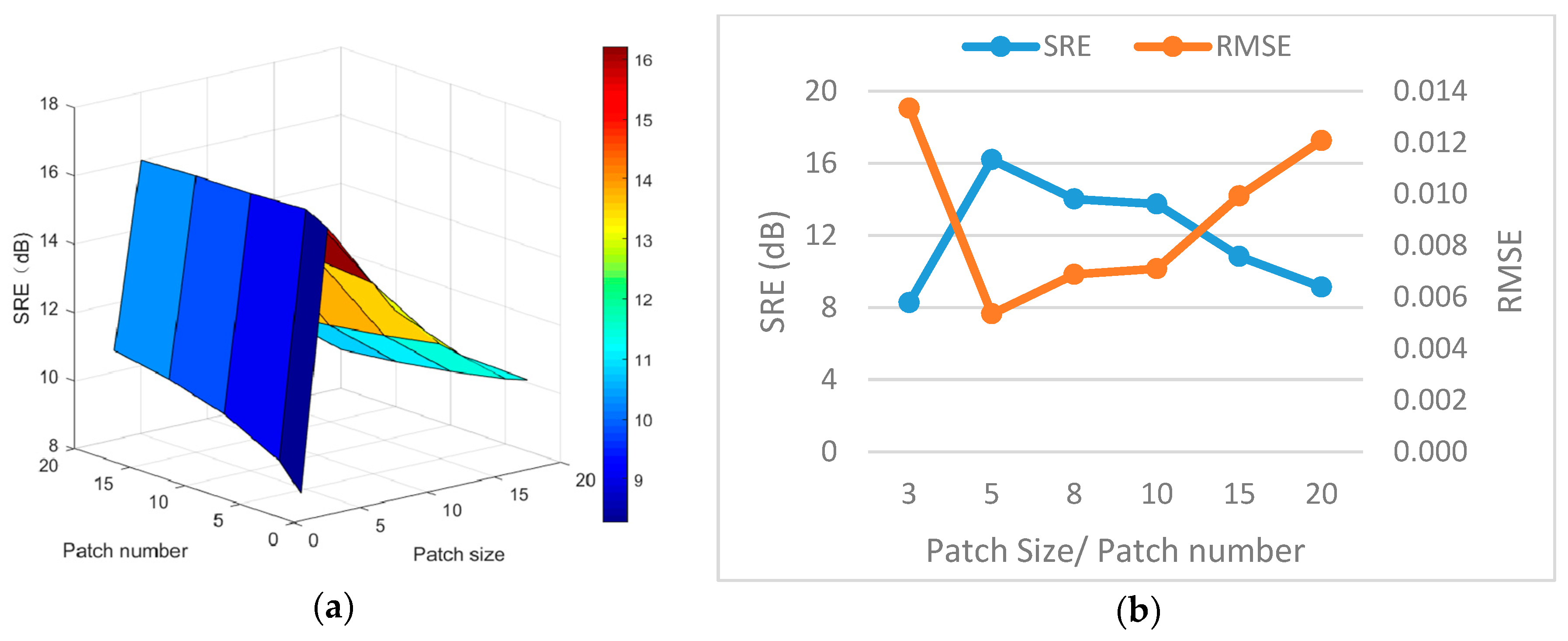
For the real hyperspectral data set experiment, we utilized the famous AVIRIS Cuprite mine map and Urban data to test the performance of the six algorithms. For the Cuprite mine map, we utilized a subset of this data set, with $250\times 191$ pixels. This subset contains 224 spectral bands between 0.4–2.5 μm. Because of the low SNR and water absorption, we removed the bands of 1-2, 105-115, 150-170, 223-224, and left 188 bands. The sub-library of USGS with 50 signatures was used to unmix this subset. Figure 10 shows the USGS mineral distribution of Cuprite in Nevada. This mineral map was drawn by Tricorder 3.3 software in 1995. However, the data for the currently published AVIRIS Cuprite mine was collected in 1997. Therefore, this mineral map was used for qualitative assessment of the six algorithms, because the mineral map product in 1995 and the AVIRIS data collected in 1997 cannot be directly compared. The Urban data has $307\times 307$ pixels and 210 spectral bands with a range of wavelengths between 0.4 and 2.5 μm. We utilized a subset with $100\times 100$ pixels for the experiment. The bands 1–4, 76, 87, 101–111, 136–153, and 198-210 have been removed because of atmospheric influence and water absorption, leaving 162 spectral bands. Since the ground truth of the Urban data set is not available, we use the abundance map obtained from [68] as the ground truth, which is obtained by the method of [69,70], including four endmembers (asphalt road, grass, tree, and roof).

Figure 11 shows the three minerals’ (Alunite, Buddingtonite and Chalcedony) abundance reconstructed by SUnSAL, CLSUnSAL, SUnSAL-TV, J-LASU, L₁-L₂ SUnSAL-TV, and NLLRSU algorithms. In Figure 11, the first row shows the mineral distribution of Alunite, Buddingtonite, and Chalcedony, which was generated by Tricorder 3.3 software in 1995 and regarded as ground truth. Although it is difficult to perform the qualitative assessment of the results from the real data produced by these algorithms, we can directly observe the results of the unmixing from the reconstructed abundance map. From Figure 11, it is clear to see that SUnSAL and CLSUnSAL perform poorly in the aspect of noise suppression while SUnSAL-TV, J-LASU, L₁-L₂ SUnSAL-TV, and NLLRSU produce smooth transition results in the edge regions because the methods with TV regularization and NLLRSU term keep structure information better than other algorithms.

Table 4. SRE and RMSE results of Urban data (The optimal results are shown in bold type).

Algorithms	SUnSAL [31]	CLSUnSAL [38]	SUnSAL-TV [42]	J-LASU [55]	L1-L2 SUnSAL-TV [43]	NLLRSU
SRE	3.9422	4.1685	4.2535	4.6928	4.5506	4.9362
RMSE	0.5534	0.5392	0.5339	0.5076	0.5160	0.4935

shows the SRE and RMSE results of the six algorithms on Urban data. Since the ground truth of Urban data cannot be obtained directly from ground measurement but obtained by an algorithm, the RMSE values of the six algorithms are much higher than those from the simulated data sets. From Table 4, it is obvious that the unmixing results obtained by the proposed algorithm are better than other state-of-the-art algorithms. The experiments on real datasets show that the nonlocal low-rank term can improve the unmixing results effectively.

4.3. Discussion

Except for the parameters, the patch size and patch number also affect the optimal results. In each patch group consisting of nonlocal patches, we utilized the nuclear norm to exploit its low-rank property. We performed several experiments to find the optimal patch size and patch number in DS1 and DS2. Figure 12a shows the effect of patch size and patch number on SRE in DS1. Figure 12b shows SRE and RMSE results as a function of patch size and patch number in DS1. After several experiments, we found the optimal patch size is $5\times 5$ pixels with 5 spectral bands and the patch number is 5. Therefore, we utilized $5\times 5\times 5$ patch size and 5 patch number for all data sets.

We conducted the experiments on the DS1 and the Cuprite mine map data set to compare the running times of the six algorithms. DS1 has $75\times 75$ pixels with 224 spectral bands and Cuprite mine map data set has $250\times 191$ pixels with 188 spectral bands. The six algorithms were performed on Intel Core i7 with 3.6 GHz and 8 GB RAM desktop computer.

Table 5. Execution time comparison (seconds/iteration).

Data	SUnSAL [31]	CLSUnSAL [38]	SUnSAL-TV [42]	J-LASU [55]	L1-L2 SUnSAL-TV [43]	NLLRSU
DS1	0.08	0.09	0.33	1.51	0.34	2.89
AVIRIS data	0.21	0.22	0.62	2.87	0.66	5.76

shows the execution time of the six algorithms. It is clear to see that the proposed algorithm (NLLRSU) takes the longest time because our method is the most complex one among the six algorithms. However, the proposed algorithm preserves the details of the abundance map best, especially when the noise level is high.

5. Conclusions

In this paper, a nonlocal low-rank sparse unmixing algorithm which explores both spectral and spatial information is proposed to improve the unmixing performance. In this method, a novel nonlocal low-rank regularization, a collaborative term and a TV term are integrated into a unified framework. The proposed model is finally solved by the ADMM algorithm effectively. Two simulated data sets and two real hyperspectral image data sets are employed to validate the superiority of the proposed method, and the experiment results show that our method outperforms several state-of-the-art methods.

In the future, we are committed to exploring better low-rank regularization to improve unmixing results more effectively. In terms of time complexity reduction, we consider employing parallel computing [71], such as multi-core CPU and GPU parallel computing, to improve computational efficiency.

References

1. Bioucas-Dias, J.M.; Plaza, A.; Dobigeon, N.; Parente, M.; Du, Q.; Gader, P.; Chanussot, J. Hyperspectral unmixing overview: Geometrical, statistical, and sparse regression-based approaches. IEEE J. Sel. Top. Appl. Earth Obs. Remote Sens. 2012, 5, 354–379. [Google Scholar] [CrossRef] [Green Version]
2. Mwaniki, M.W.; Matthias, M.S.; Schellmann, G. Application of remote sensing technologies to map the structural geology of central region of kenya. IEEE J. Sel. Top. Appl. Earth Obs. Remote Sens. 2015, 8, 1855–1867. [Google Scholar] [CrossRef]
3. Yang, S.; Shi, Z. Hyperspectral image target detection improvement based on total variation. IEEE. Trans. Image Process. 2016, 25, 2249–2258. [Google Scholar] [CrossRef] [PubMed]
4. Li, H.; Liu, J.; Yu, H. An automatic sparse pruning endmember extraction algorithm with a combined minimum volume and deviation constraint. Remote Sens. 2018, 10, 32. [Google Scholar] [CrossRef] [Green Version]
5. Jiao, C.; Chen, C.; McGarvey, R.G.; Bohlman, S.; Jiao, L.; Zare, A. Multiple instance hybrid estimator for hyperspectral target characterization and sub-pixel target detection. ISPRS-J. Photogramm. Remote Sens. 2018, 146, 235–250. [Google Scholar] [CrossRef] [Green Version]
6. Wang, X.; Zhong, Y.; Xu, Y.; Zhang, L.; Xu, Y. Saliency-based endmember detection for hyperspectral imagery. IEEE. Trans. Geosci. Remote Sens. 2018, 56, 3667–3680. [Google Scholar] [CrossRef]
7. Xu, X.; Shi, Z.; Pan, B. A supervised abundance estimation method for hyperspectral unmixing. Remote Sens. Lett. 2018, 9, 383–392. [Google Scholar] [CrossRef]
8. Bashir, S.; Carter, E.M. Robust mixture of linear regression models. Commun. Stat. Theory Methods 2012, 41, 3371–3388. [Google Scholar] [CrossRef]
9. Shi, C.; Wang, L. Linear spatial spectral mixture model. IEEE. Trans. Geosci. Remote Sens. 2016, 54, 3599–3611. [Google Scholar] [CrossRef]
10. Ahmed, A.M.; Duran, O.; Zweiri, Y.; Smith, M. Hybrid spectral unmixing: Using artificial neural networks for linear/non-linear switching. Remote Sens. 2017, 9, 22. [Google Scholar] [CrossRef] [Green Version]
11. Li, C.; Liu, Y.; Cheng, J.; Song, R.; Peng, H.; Chen, Q.; Chen, X. Hyperspectral unmixing with bandwise generalized bilinear model. Remote Sens. 2018, 10, 19. [Google Scholar] [CrossRef] [Green Version]
12. Marinoni, A.; Plaza, A.; Gamba, P. Harmonic mixture modeling for efficient nonlinear hyperspectral unmixing. IEEE J. Sel. Top. Appl. Earth Obs. Remote Sens. 2016, 9, 4247–4256. [Google Scholar] [CrossRef]
13. Nascimento, J.M.P.; Dias, J.M.B. Vertex component analysis: A fast algorithm to unmix hyperspectral data. IEEE. Trans. Geosci. Remote Sens. 2005, 43, 898–910. [Google Scholar] [CrossRef] [Green Version]
14. Guo, J.; Li, Y.; Liu, K.; Lei, J.; Wang, K. Fast FPGA implementation for computing the pixel purity index of hyperspectral images. J. Circuits Syst. Comput. 2018, 27, 10. [Google Scholar] [CrossRef]
15. Wu, C.; Chen, H.; Chang, C. Real-time N-finder processing algorithms for hyperspectral imagery. J. Real-Time Image Process. 2012, 7, 105–129. [Google Scholar] [CrossRef] [Green Version]
16. Zhang, S.; Agathos, A.; Li, J. Robust minimum volume simplex analysis for hyperspectral unmixing. IEEE. Trans. Geosci. Remote Sens. 2017, 55, 6431–6439. [Google Scholar] [CrossRef]
17. Geng, X.; Ji, L.; Yang, W.; Ling, C. The multiplicative update rule for an extension of the iterative constrained endmembers algorithm. Int. J. Remote Sens. 2017, 38, 7457–7467. [Google Scholar] [CrossRef]
18. Zhou, G.X.; Xie, S.L.; Yang, Z.Y.; Yang, J.M.; He, Z.S. Minimum-volume-constrained nonnegative matrix factorization: Enhanced sbility of learning parts. IEEE. Trans. Neural Netw. 2011, 22, 1626–1637. [Google Scholar] [CrossRef]
19. Li, J.; Bioucas-Dias, J.M.; Plaza, A.; Liu, L. Robust collaborative nonnegative matrix factorization for hyperspectral unmixing. IEEE. Trans. Geosci. Remote Sens. 2016, 54, 6076–6090. [Google Scholar] [CrossRef] [Green Version]
20. Li, X.; Jia, X.; Wang, L.; Zhao, K. Reduction of spectral unmixing uncertainty using minimum-class-variance support vector machines. IEEE. Geosci. Remote Sens. Lett. 2016, 13, 1335–1339. [Google Scholar] [CrossRef]
21. Chen, Y.; Xiong, J.; Xu, W.; Zuo, J. A novel online incremental and decremental learning algorithm based on variable support vector machine. Cluster Comput. 2019, 22, 7435–7445. [Google Scholar] [CrossRef]
22. Chen, Y.; Xu, W.; Zuo, J.; Yang, K. The fire recognition algorithm using dynamic feature fusion and IV-SVM classifier. Clust. Comput. 2019, 22, 7665–7675. [Google Scholar] [CrossRef]
23. Tu, Y.; Lin, Y.; Wang, J.; Kim, J.U. Semi-supervised learning with generative adversarial networks on digital signal modulation classification. Comput. Mater. Contin. 2018, 55, 243–254. [Google Scholar]
24. Meng, R.; Rice, S.; Wang, J.; Sun, X. A fusion steganographic algorithm based on faster R-CNN. Comput. Mater. Contin. 2018, 55, 1–16. [Google Scholar]
25. Long, M.; Zeng, Y. Detecting iris liveness with batch normalized convolutional neural network. Comput. Mater. Contin. 2019, 58, 493–504. [Google Scholar] [CrossRef]
26. Cheng, G.; Zhou, P.C.; Han, J.W. Learning rotation-invariant convolutional neural networks for object detection in VHR optical remote sensing images. IEEE. Trans. Geosci. Remote Sens. 2016, 54, 7405–7415. [Google Scholar] [CrossRef]
27. Zhang, J.; Jin, X.; Sun, J.; Wang, J.; Sangaiah, A.K. Spatial and semantic convolutional features for robust visual object tracking. Multimed. Tools Appl. 2018, 1, 1–21. [Google Scholar] [CrossRef]
28. Zeng, D.; Dai, Y.; Li, F.; Wang, J.; Kumar, A. Aspect based sentiment analysis by a linguistically regularized CNN with gated mechanism. J. Intell. Fuzzy Syst. 2019, 36, 3971–3980. [Google Scholar] [CrossRef]
29. Licciardi, G.A.; Frate, F.D. Pixel unmixing in hyperspectral data by means of neural networks. IEEE. Trans. Geosci. Remote Sens. 2011, 49, 4163–4172. [Google Scholar] [CrossRef]
30. Chen, Y.; Jiang, H.; Li, C.; Jia, X.; Ghamisi, P. Deep feature extraction and classification of hyperspectral images based on convolutional neural networks. IEEE. Trans. Geosci. Remote Sens. 2016, 54, 6232–6251. [Google Scholar] [CrossRef] [Green Version]
31. Iordache, M.D.; Bioucas-Dias, J.M.; Plaza, A. Sparse unmixing of hyperspectral data. IEEE. Trans. Geosci. Remote Sens. 2011, 49, 2014–2039. [Google Scholar] [CrossRef] [Green Version]
32. Chen, X.H.; Chen, J.; Jia, X.P.; Somers, B.; Wu, J.; Coppin, P. A quantitative analysis of virtual endmembers’ increased impact on the collinearity effect in spectral unmixing. IEEE. Trans. Geosci. Remote Sens. 2011, 49, 2945–2956. [Google Scholar] [CrossRef]
33. Song, Y.; Yang, G.; Xie, H.; Zhang, D.; Sun, X. Residual domain dictionary learning for compressed sensing video recovery. Multimed. Tools Appl. 2017, 76, 10083–10096. [Google Scholar] [CrossRef]
34. He, S.L.Z.; Tang, Y.; Liao, Z.; Wang, J.; Kim, H.J. Parameters compressing in deep learning. Comput. Mater. Contin. 2019, 1–16. [Google Scholar]
35. Clark, R.N.; Swayze, G.A.; Wise, R.A.; Livo, K.E.; Hoefen, T.M.; Kokaly, R.F.; Sutley, S.J. USGS Digital Spectral Library Splib06a; U.S. Geological Survey: Reston, VA, USA, 2007; p. 231.
36. Yuan, J.; Zhang, Y.; Gao, F. An overview on linear hyperspectral unmixing. J. Infrared Millim. Waves 2018, 37, 553–571. [Google Scholar]
37. Eckstein, J.; Bertsekas, D.P. On the Douglas-Rachford splitting method and the proximal point algorithm for maximal monotone operators. Math. Program. 1992, 55, 293–318. [Google Scholar] [CrossRef] [Green Version]
38. Iordache, M.D.; Bioucas-Dias, J.M.; Plaza, A. Collaborative sparse regression for hyperspectral unmixing. IEEE. Trans. Geosci. Remote Sens. 2014, 52, 341–354. [Google Scholar] [CrossRef] [Green Version]
39. Tang, W.; Shi, Z.; Wu, Y.; Zhang, C. Sparse unmixing of hyperspectral data using spectral a priori information. IEEE. Trans. Geosci. Remote Sens. 2015, 53, 770–783. [Google Scholar] [CrossRef]
40. Zhang, S.Q.; Li, J.; Liu, K.; Deng, C.Z.; Liu, L.; Plaza, A. Hyperspectral unmixing based on local collaborative sparse regression. IEEE. Geosci. Remote Sens. Lett. 2016, 13, 631–635. [Google Scholar] [CrossRef]
41. Li, S.; Kang, X.; Fang, L.; Hu, J.; Yin, H. Pixel-level image fusion: A survey of the state of the art. Inf. Fusion 2017, 33, 100–112. [Google Scholar] [CrossRef]
42. Iordache, M.D.; Bioucas-Dias, J.M.; Plaza, A. Total variation spatial regularization for sparse hyperspectral unmixing. IEEE. Trans. Geosci. Remote Sens. 2012, 50, 4484–4502. [Google Scholar] [CrossRef] [Green Version]
43. Sun, L.; Ge, W.; Chen, Y.; Zhang, J.; Jeon, B. Hyperspectral unmixing employing l(1)–l(2) sparsity and total variation regularization. Int. J. Remote Sens. 2018, 39, 6037–6060. [Google Scholar] [CrossRef]
44. Qu, Q.; Nasrabadi, N.M.; Tran, T.D. Abundance estimation for bilinear mixture models via joint sparse and low-rank representation. IEEE. Trans. Geosci. Remote Sens. 2014, 52, 4404–4423. [Google Scholar]
45. Zhang, H.; He, W.; Zhang, L.; Shen, H.; Yuan, Q. Hyperspectral image restoration using low-rank matrix recovery. IEEE. Trans. Geosci. Remote Sens. 2014, 52, 4729–4743. [Google Scholar] [CrossRef]
46. He, W.; Zhang, H.; Zhang, L.; Shen, H. Total-variation-regularized low-rank matrix factorization for hyperspectral image restoration. IEEE. Trans. Geosci. Remote Sens. 2016, 54, 176–188. [Google Scholar] [CrossRef]
47. Zhao, Y.Q.; Yang, J.X. Hyperspectral image denoising via sparse representation and low-rank constraint. IEEE. Trans. Geosci. Remote Sens. 2015, 53, 296–308. [Google Scholar] [CrossRef]
48. Chang, Y.; Yan, L.; Zhong, S. Hyper-Laplacian regularized unidirectional low-rank tensor recovery for multispectral image denoising. In Proceedings of the IEEE Conference on Computer Vision and Pattern Recognition (CVPR), Honolulu, HI, USA, 21–26 July 2017; pp. 5901–5909. [Google Scholar]
49. Sun, L.; Ma, C.; Chen, Y.; Shim, H.J.; Wu, Z.; Jeon, B. Adjacent superpixel-based multiscale spatial-spectral kernel for hyperspectral classification. IEEE J. Sel. Top. Appl. Earth Observ. Remote Sens. 2019, 12, 1905–1919. [Google Scholar] [CrossRef]
50. Sun, L.; Ma, C.; Chen, Y.; Zheng, Y.; Shim, H.J.; Wu, Z.; Jeon, B. Low rank component Induced spatial-spectral kernel method for hyperspectral image classification. IEEE Trans. Circuits Syst. Video Technol. 2019, 26, 613–626. [Google Scholar] [CrossRef]
51. Chen, Y.; Xia, R.; Wang, Z.; Zhang, J.; Yang, K.; Cao, Z. The visual saliency detection algorithm research based on hierarchical principle component analysis method. Multimed. Tools Appl. 2019, 75, 16943–16958. [Google Scholar] [CrossRef]
52. Yang, J.; Zhao, Y.; Chan, J.; Kong, S. Coupled sparse denoising and unmixing with low-rank constraint for hyperspectral image. IEEE. Trans. Geosci. Remote Sens. 2016, 54, 1818–1833. [Google Scholar] [CrossRef]
53. Giampouras, P.V.; Themelis, K.E.; Rontogiannis, A.A.; Koutroumbas, K.D. Simultaneously sparse and low-rank abundance matrix estimation for hyperspectral image unmixing. IEEE. Trans. Geosci. Remote Sens. 2016, 54, 4775–4789. [Google Scholar] [CrossRef] [Green Version]
54. Mei, X.; Ma, Y.; Li, C.; Fan, F.; Huang, J.; Ma, J. Robust GBM hyperspectral image unmixing with superpixel segmentation based low rank and sparse representation. Neurocomputing 2018, 275, 2783–2797. [Google Scholar] [CrossRef]
55. Rizkinia, M.; Okuda, M. Joint local abundance sparse unmixing for hyperspectral images. Remote Sens. 2017, 9, 22. [Google Scholar] [CrossRef] [Green Version]
56. Dabov, K.; Foi, A.; Katkovnik, V.; Egiazarian, K. Image denoising by sparse 3-D transform-domain collaborative filtering. IEEE. Trans. Image Process. 2007, 16, 2080–2095. [Google Scholar] [CrossRef] [PubMed]
57. Bioucas-Dias, J.M. A variable splitting augmented Lagrangian approach to linear spectral unmixing. In Proceedings of the First Workshop on Hyperspectral Image and Signal Processing: Evolution in Remote Sensing, Grenoble, France, 26–28 August 2009; pp. 1–4. [Google Scholar]
58. Zhang, X.R.; Li, C.; Zhang, J.Y.; Chen, Q.M.; Feng, J.; Jiao, L.C.; Zhou, H.Y. Hyperspectral unmixing via low-rank representation with space consistency constraint and spectral library pruning. Remote Sens. 2018, 10, 21. [Google Scholar] [CrossRef] [Green Version]
59. Lou, Y.; Yin, P.; He, Q.; Xin, J. Computing sparse representation in a highly coherent dictionary based on difference of l1 and l2. J. Sci. Comput. 2015, 64, 178–196. [Google Scholar] [CrossRef]
60. Sun, L.; Wu, Z.; Liu, J.; Xiao, L.; Wei, Z. Supervised spectral-spatial hyperspectral image classification with weighted markov random fields. IEEE. Trans. Geosci. Remote Sens. 2015, 53, 1490–1503. [Google Scholar] [CrossRef]
61. Bruckstein, A.M.; Elad, M.; Zibulevsky, M. On the uniqueness of nonnegative sparse solutions to underdetermined systems of equations. IEEE. Trans. Inf. Theory 2008, 54, 4813–4820. [Google Scholar] [CrossRef]
62. Wright, S.J.; Nowak, R.D.; Figueiredo, M.A.T. Sparse reconstruction by separable approximation. IEEE. Trans. Signal Process. 2009, 57, 2479–2493. [Google Scholar] [CrossRef] [Green Version]
63. Vinchurkar, P.P.; Rathkanthiwar, S.V.; Kakde, S.M. HDL Implementation of DFT Architectures Using Winograd Fast Fourier Transform Algorithm. In Proceedings of the Fifth International Conference on Communication Systems and Network Technologies (CSNT), Gwalior, India, 4–6 April 2015; pp. 397–401. [Google Scholar]
64. Combettes, P.L.; Wajs, V.R. Signal recovery by proximal forward-backward splitting. Multiscale Model. Simul. 2005, 4, 1168–1200. [Google Scholar] [CrossRef] [Green Version]
65. USGS Digital Spectral Library 06. Available online: https://speclab.cr.usgs.gov/spectral.lib06 (accessed on 8 June 2016).
66. Altmann, Y.; Pereyra, M.; Bioucas-Dias, J.M. Collaborative sparse regression using spatially correlated supports-application to hyperspectral unmixing. IEEE. Trans. Image Process. 2015, 24, 12. [Google Scholar] [CrossRef] [PubMed] [Green Version]
67. Guerra, R.; Santos, L.; Lopez, S.; Sarmiento, R. A new fast algorithm for linearly unmixing hyperspectral images. IEEE. Trans. Geosci. Remote Sens. 2015, 53, 6752–6765. [Google Scholar] [CrossRef]
68. Datasets & Ground Truths. Available online: http://www.escience.cn/people/feiyunZHU/Dataset_GT.html (accessed on 8 November 2019).
69. Zhu, F.Y.; Wang, Y.; Fan, B.; Xiang, S.M.; Meng, G.F.; Pan, C.H. Spectral unmixing via data-guided sparsity. IEEE Trans. Image Process. 2014, 23, 5412–5427. [Google Scholar] [CrossRef] [PubMed] [Green Version]
70. Zhu, F.Y.; Wang, Y.; Xiang, S.M.; Fan, B.; Pan, C.H. Structured sparse method for hyperspectral unmixing. ISPRS-J. Photogramm. Remote Sens. 2014, 88, 101–118. [Google Scholar] [CrossRef] [Green Version]
71. Jiang, Y.; Zhao, M.; Hu, C.; He, L.; Bai, H.; Wang, J. A parallel FP-growth algorithm on World Ocean Atlas data with multi-core CPU. J. Supercomput. 2019, 75, 732–745. [Google Scholar] [CrossRef]
Figure 1. The flow chart of the proposed unmixing algorithm.
Remotesensing 11 02897 g001
Figure 2. The process of obtaining the patch group and the nonlocal abundance matrix of the patch group. In the 3D form of abundance data, the small red box denotes a key patch, which slides across all dimensions in abundance data. The small blue boxes denote r number of similar patches. Then we stack all r+1 patches to a patch group and convert this patch group into the vectors to obtain the abundance matrix.
Remotesensing 11 02897 g002
Figure 3. True fractional abundances of endmembers in the simulated data set 1 (DS1). (a) Simulated image; (b) endmember 1; (c) endmember 2; (d) endmember 3; (e) endmember 4; (f) endmember 5.
Remotesensing 11 02897 g003
Figure 4. True fractional abundances of endmembers in the simulated data set 2 (DS2). (a) Endmember 1; (b) endmember 2; (c) endmember 3; (d) endmember 4; (e) endmember 5; (f) endmember 6; (g) endmember 7; (h) endmember 8; (i) endmember 9.
Remotesensing 11 02897 g004aRemotesensing 11 02897 g004b
Figure 5. Signal reconstruction error (SRE)(dB) as a function of parameters λ , λ T V , and λ N L for DS1 with 20dB SNR level. (a) λ and λ T V ; (b) λ and λ N L ; (c) λ T V and λ N L .
Remotesensing 11 02897 g005
Figure 6. Reconstructed fractional abundances of endmember 1 in DS1 with 20dB SNR level. (a) SUnSAL; (b) CLSUnSAL; (c) SUnSAL-TV; (d) J-LASU; (e) L1-L2 SUnSAL-TV; (f) NLLRSU.
Remotesensing 11 02897 g006
Figure 7. Reconstructed fractional abundances of endmember 5 in DS1 with 20dB SNR level. (a) SUnSAL; (b) CLSUnSAL; (c) SUnSAL-TV; (d) J-LASU; (e) L1-L2 SUnSAL-TV; (f) NLLRSU.
Remotesensing 11 02897 g007
Figure 8. Reconstructed fractional abundances of endmember 5 in DS2 with 20dB SNR level. (a) SUnSAL; (b) CLSUnSAL; (c) SUnSAL-TV; (d) J-LASU; (e) L1-L2 SUnSAL-TV; (f) NLLRSU.
Remotesensing 11 02897 g008
Figure 9. Reconstructed fractional abundances of endmember 9 in DS2 with 20dB SNR level. (a) SUnSAL; (b) CLSUnSAL; (c) SUnSAL-TV; (d) J-LASU; (e) L1-L2 SUnSAL-TV; (f) NLLRSU.
Remotesensing 11 02897 g009aRemotesensing 11 02897 g009b
Figure 10. United States Geological Survey (USGS) mineral map of Cuprite in Nevada.
Remotesensing 11 02897 g010
Figure 11. The first row (ac) shows the distribution maps of Alunite, Buddingtonite, and Chalcedony (column 1-3) by Tricorder software. The second row (du) to the seventh row shows the reconstructed abundances maps of three minerals by SUnSAL, CLSUnSAL, SUnSAL-TV, J-LASU, L1-L2 SUnSAL-TV, NLLRSU.
Remotesensing 11 02897 g011
Figure 12. (a) Effect of patch size and number on SRE; (b) SRE and RMSE result with patch size and patch number change.
Remotesensing 11 02897 g012