Deriving Particulate Organic Carbon in Coastal Waters from Remote Sensing: Inter-Comparison Exercise and Development of a Maximum Band-Ratio Approach

 , ,
, , 
Abstract
1. Introduction
2. Data and Methods
2.1. In Situ Data
2.2. Satellite-In Situ Matchup Data Base
2.3. Candidate Algorithms
2.3.1. Band Ratio-based Algorithms
2.3.2. Absolute Rrs-based Algorithms
2.3.3. Color Index Algorithm
2.4. Statistical Indicators Used for Model Development and Validation
3. Results and Discussion
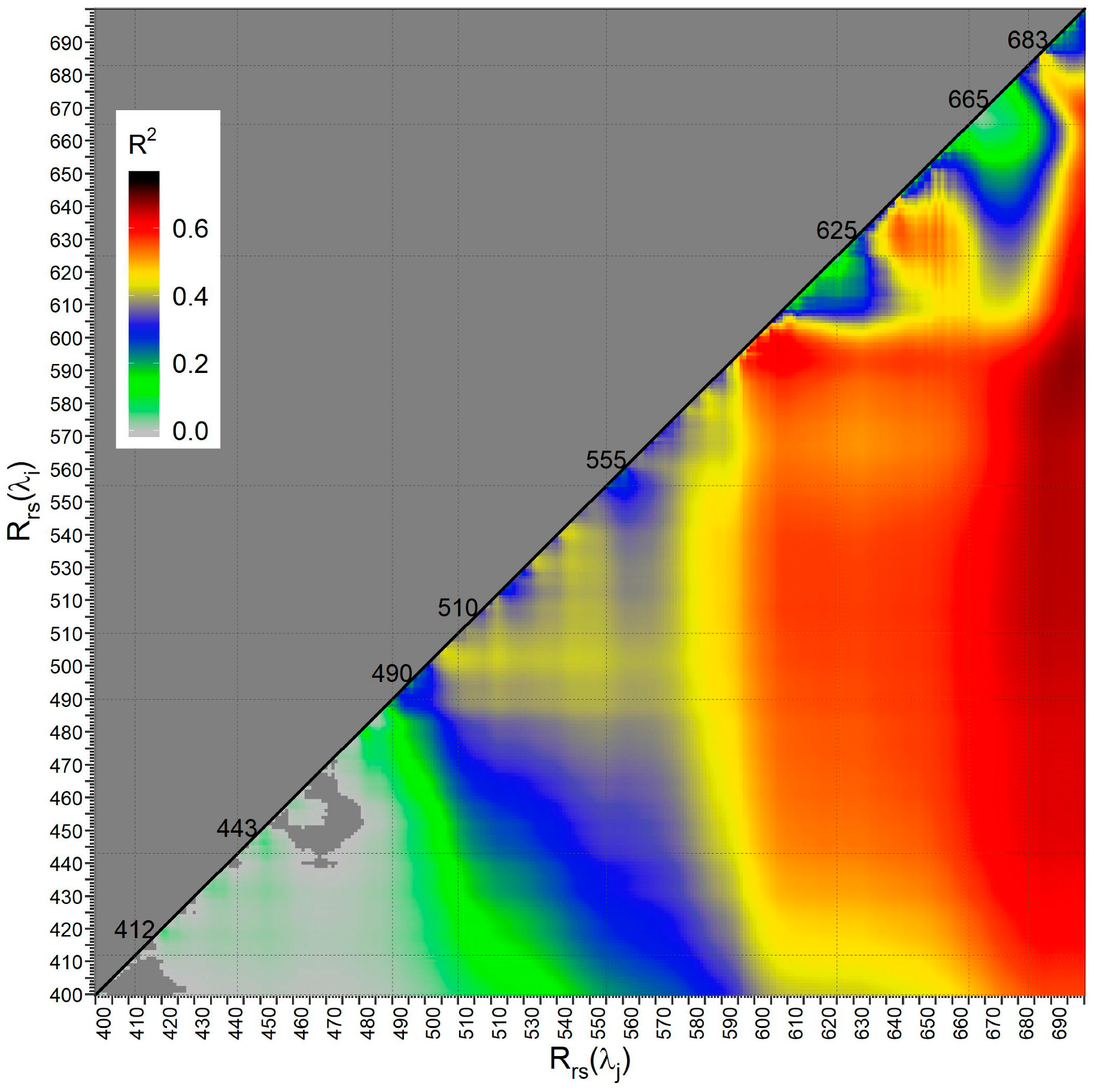
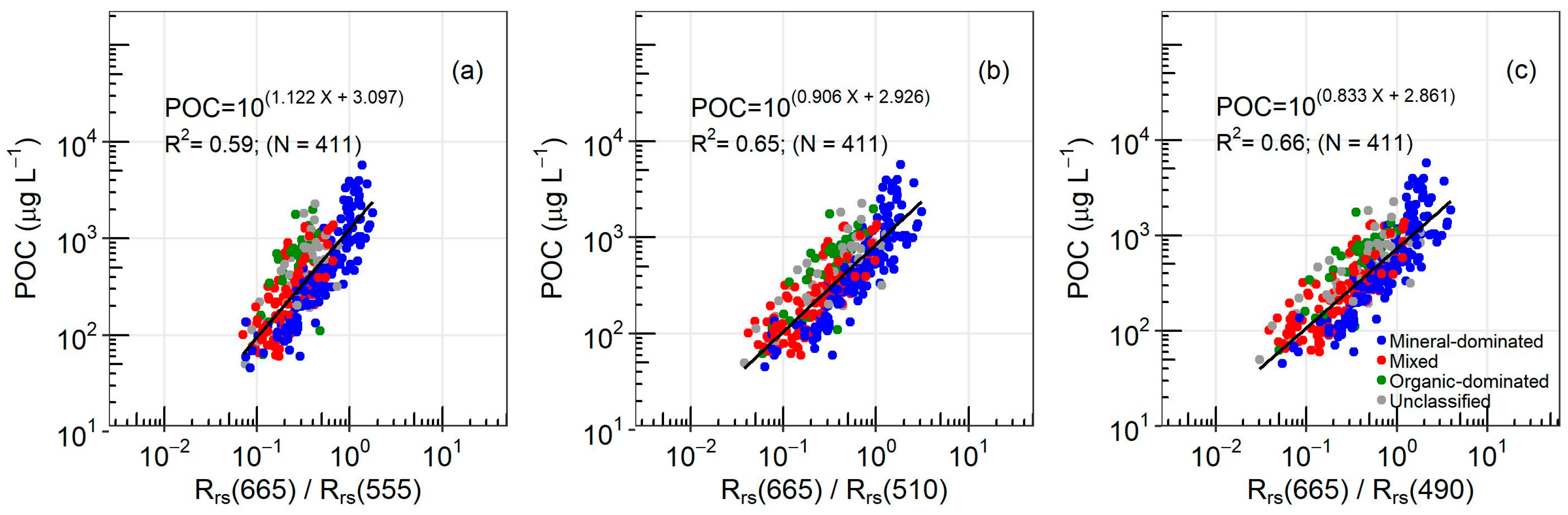
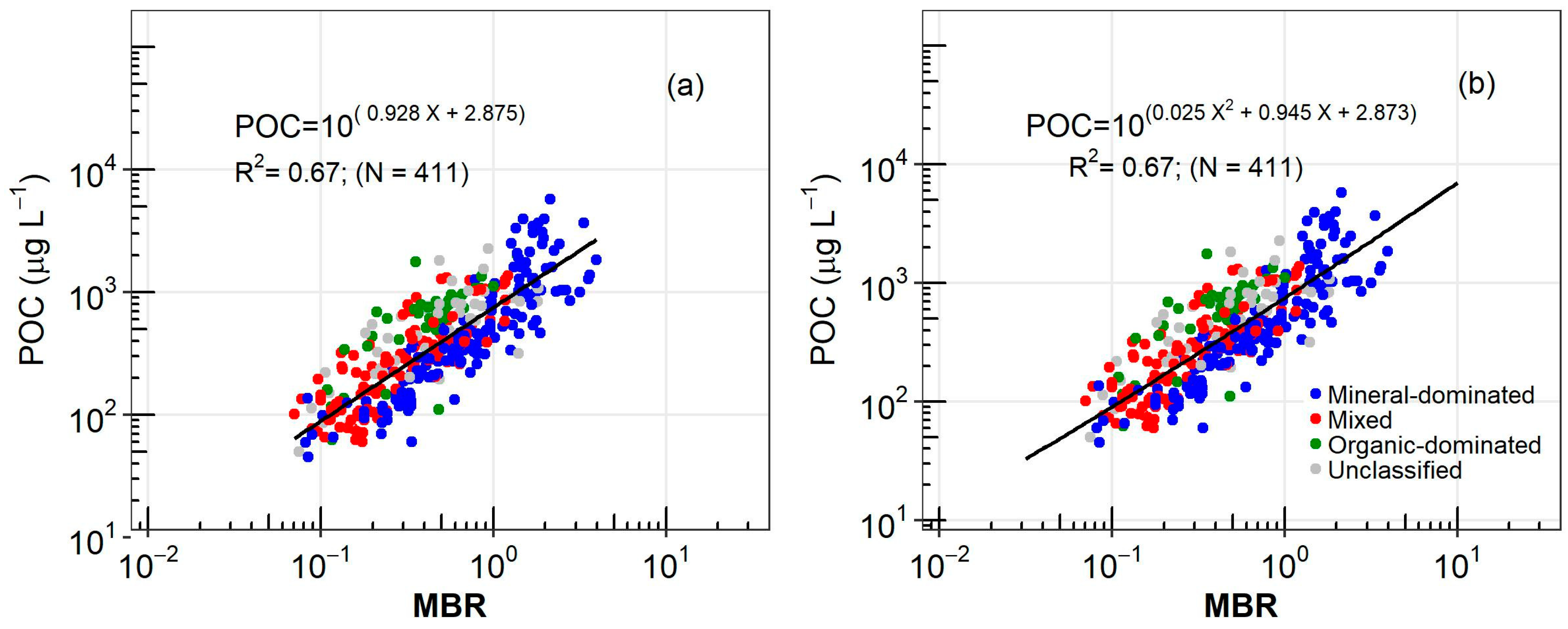
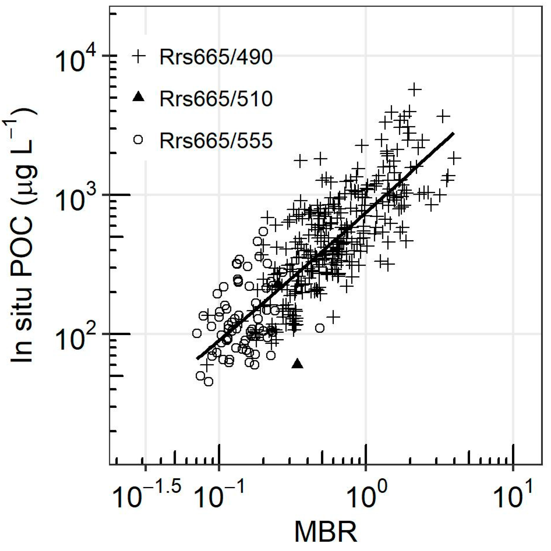
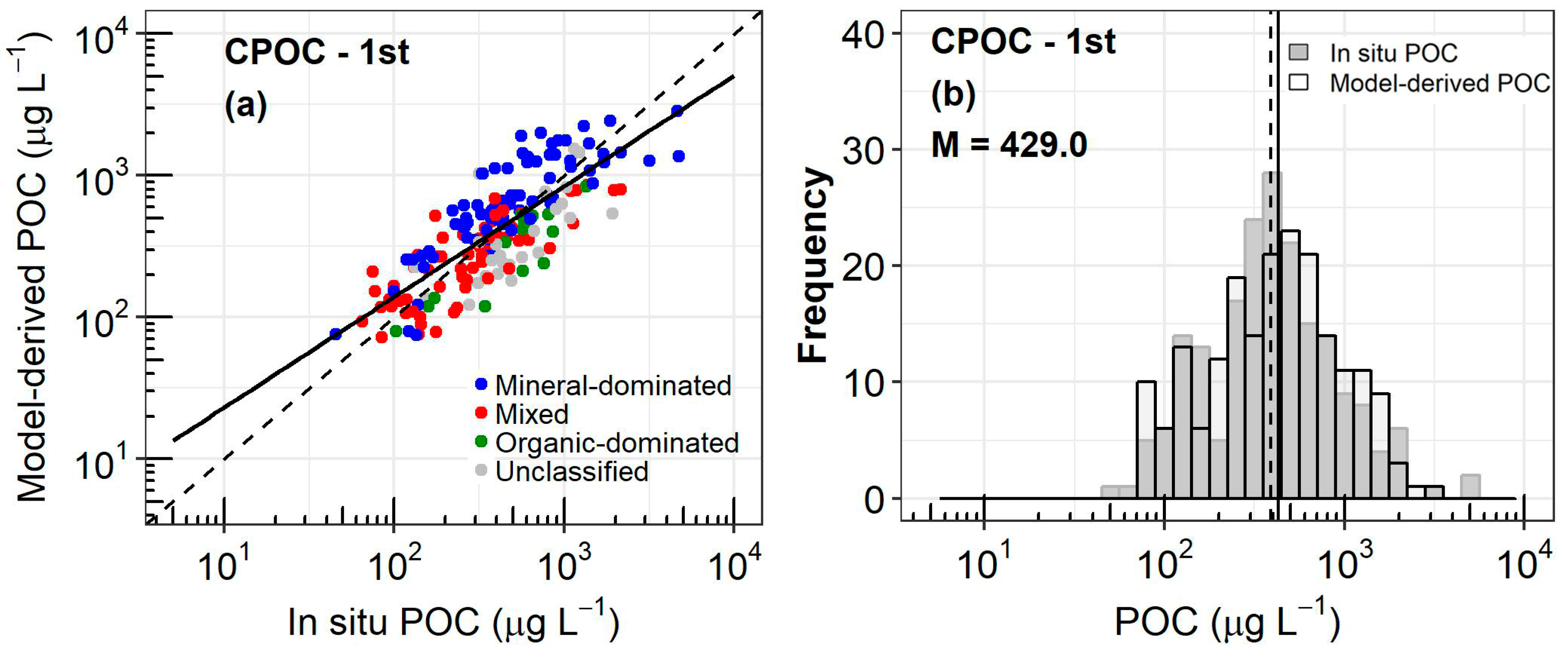
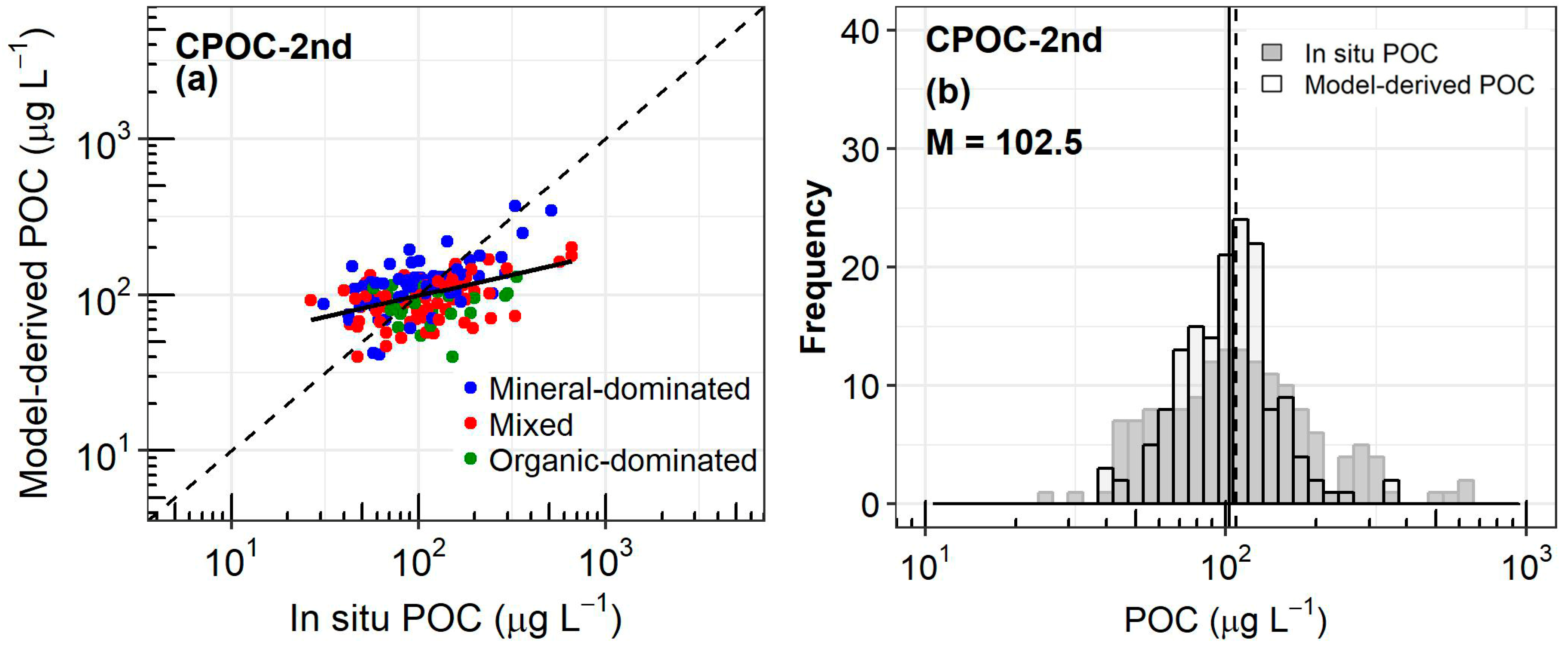
3.1. Development of a New Algorithm for POC
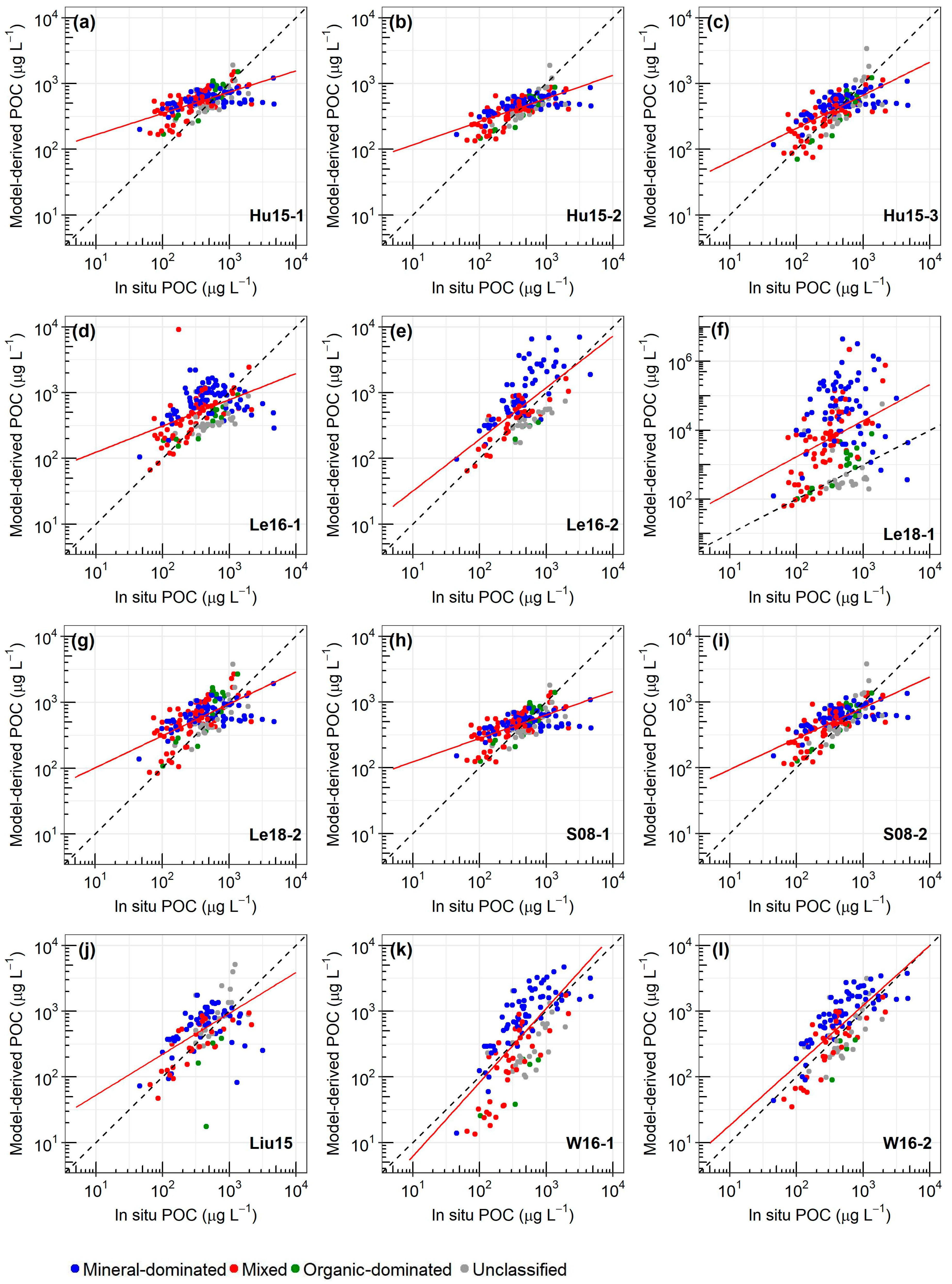
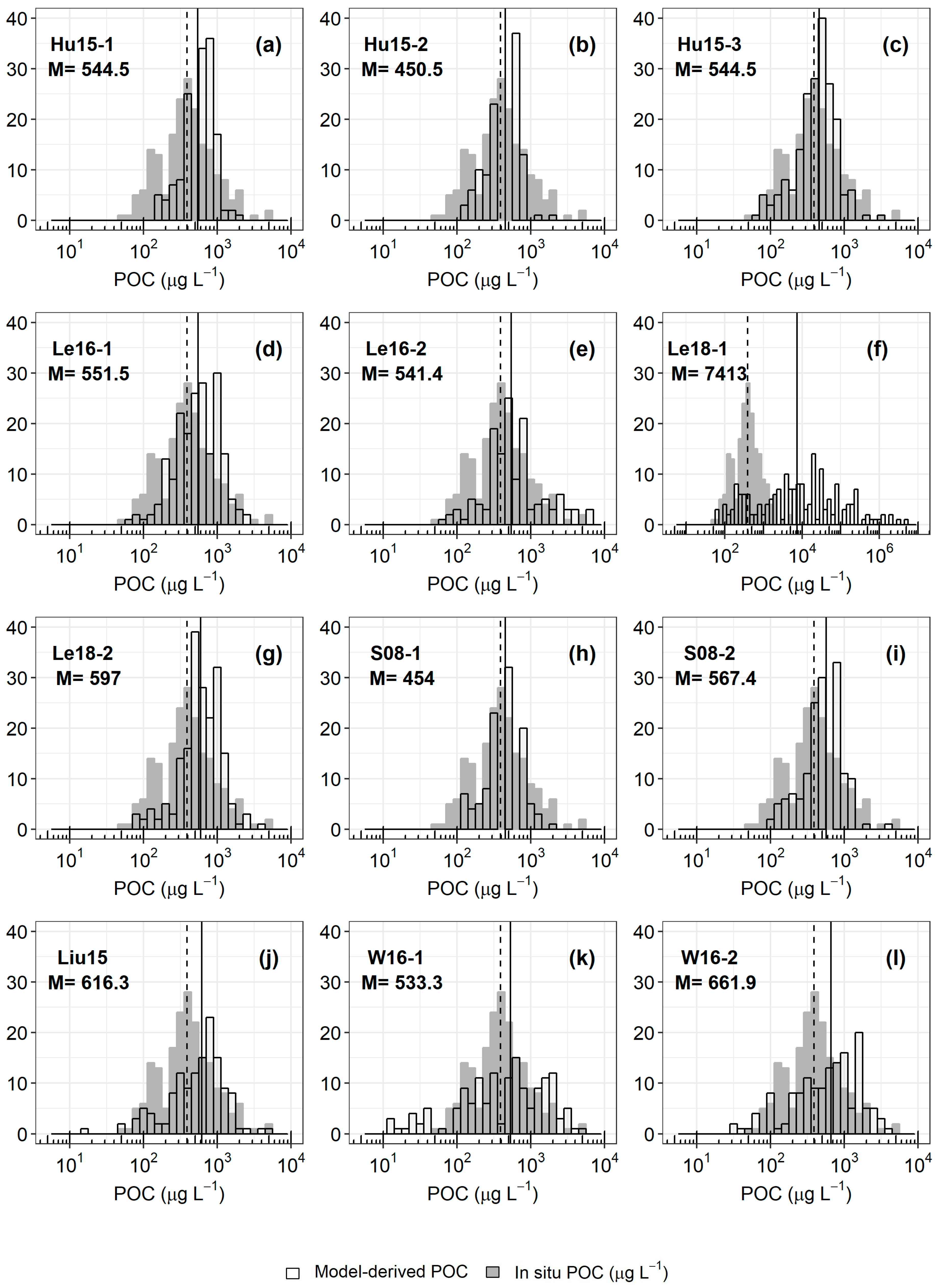
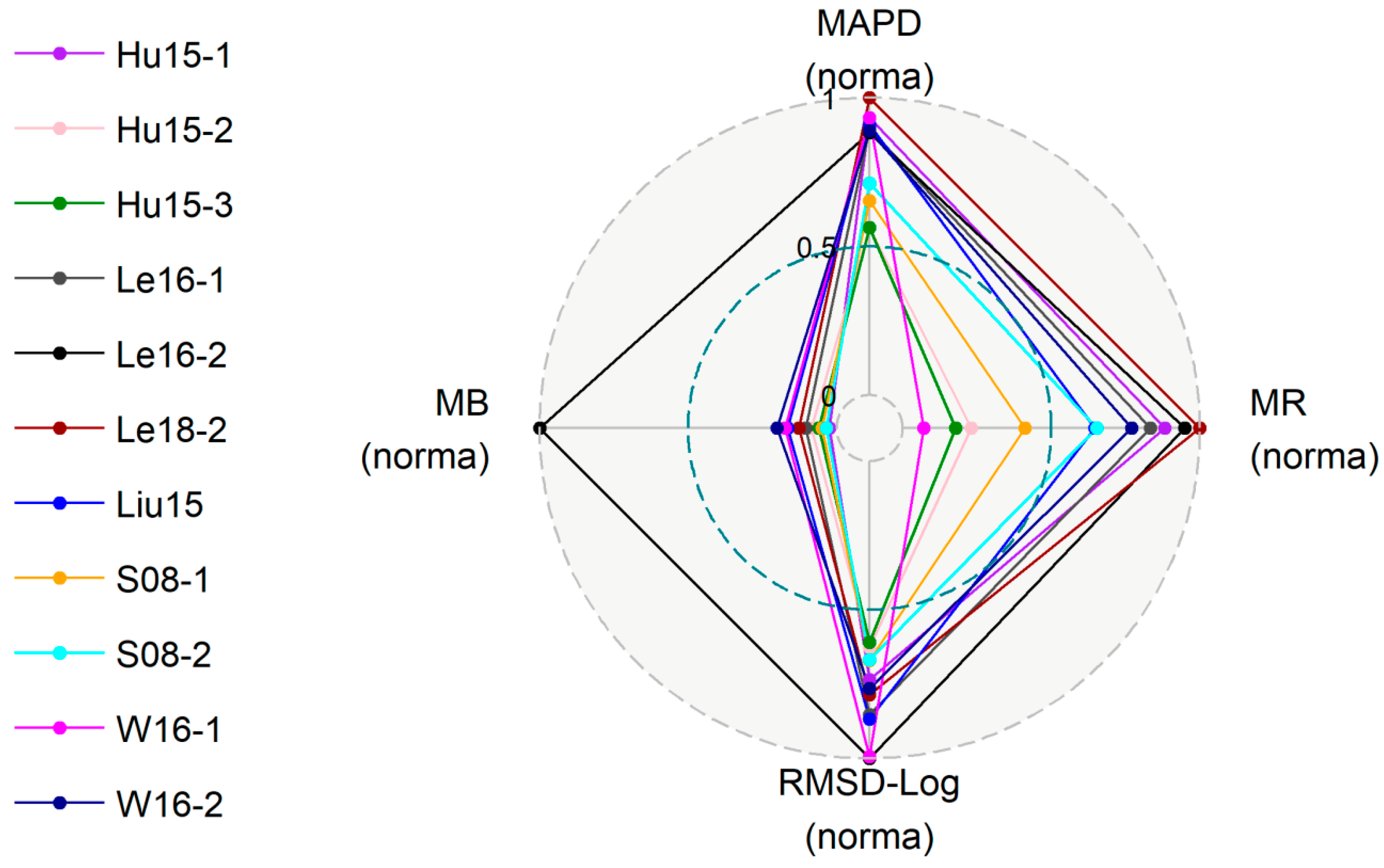
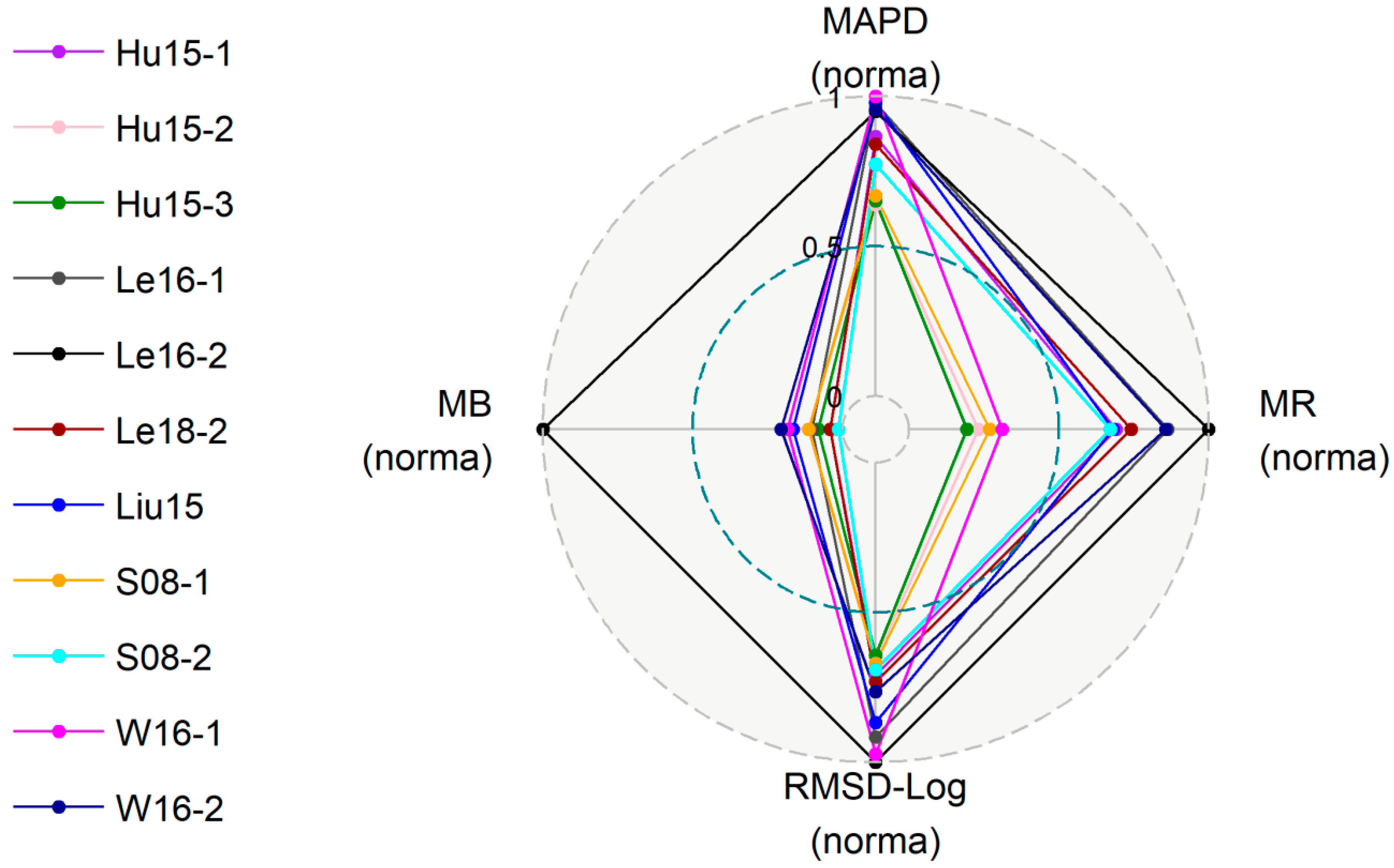
3.2. Inter-comparison Exercise of Existing Algorithms
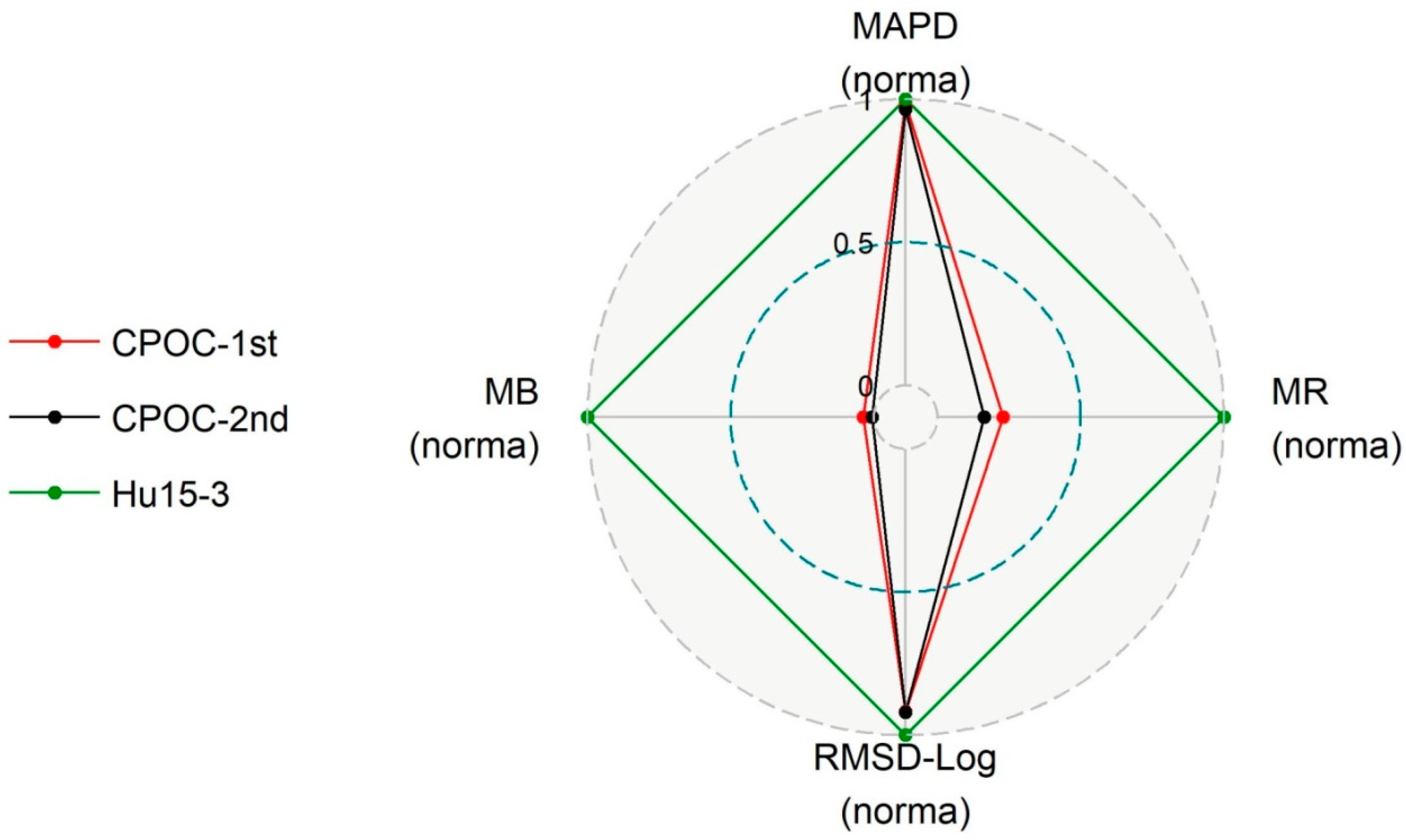
3.3. Performance of the New Algorithms
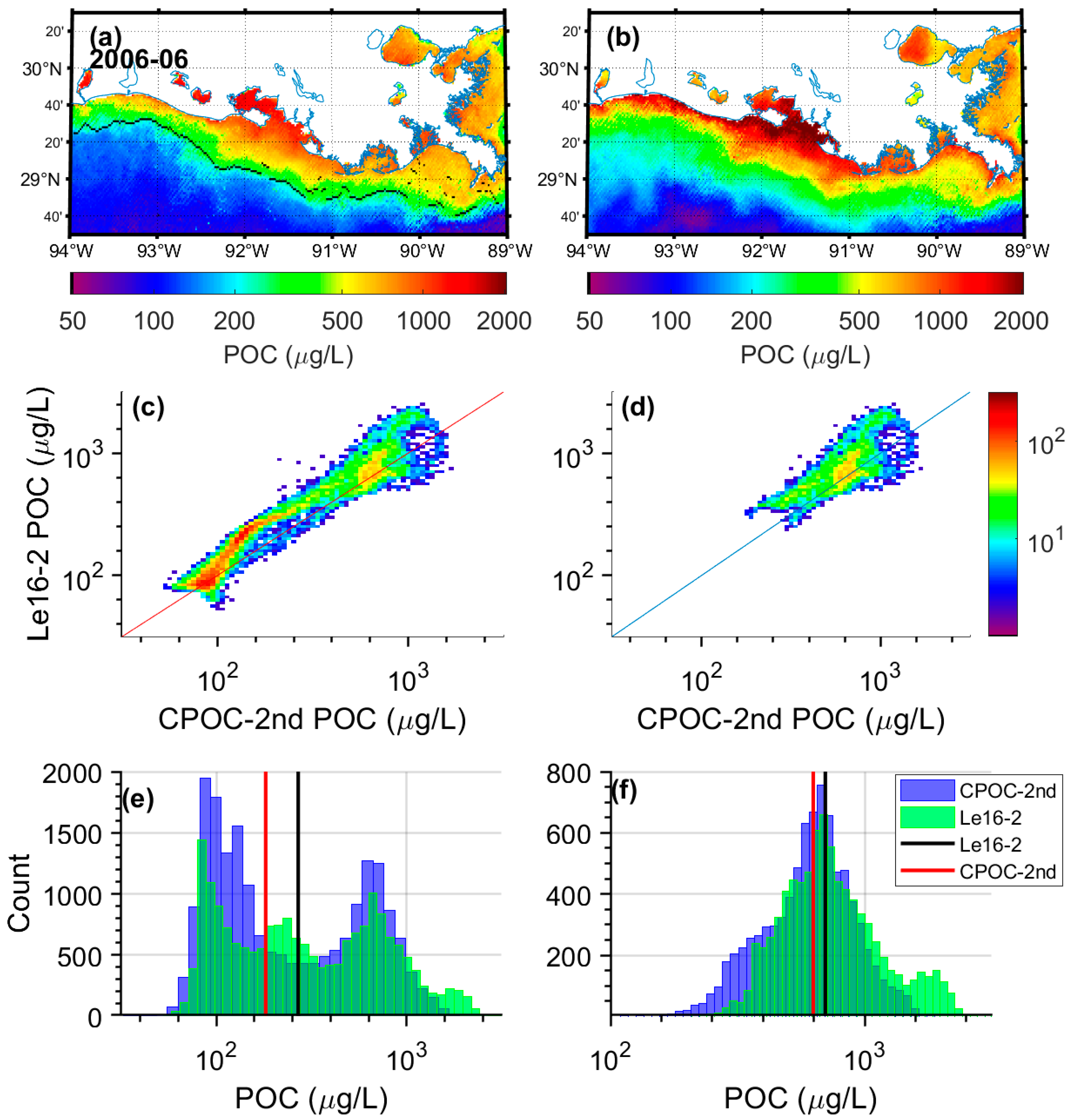
3.4. Satellite POC Estimates for Coastal Regions
4. Concluding Remarks
Author Contributions
Funding
Acknowledgments
Conflicts of Interest
Appendix A

| Algorithms | N | MAPD | MB | RMSDlog | RMSD | MR | R2 | Slope | Intercept | Negative Value |
|---|---|---|---|---|---|---|---|---|---|---|
| Hu15-1 | 144 | 55.44 | −50.55 | 0.31 | 651.0 | 1.41 | 0.37 | 0.28 | 1.98 | 0 |
| Hu15-2 | 144 | 41.01 | −142.6 | 0.29 | 666.9 | 1.14 | 0.41 | 0.31 | 1.82 | 0 |
| Hu15-3 | 144 | 41.77 | −101.3 | 0.28 | 677.6 | 1.11 | 0.41 | 0.44 | 1.48 | 0 |
| Le16-1 | 144 | 62.68 | 126.8 | 0.4 | 1084 | 1.51 | 0.14 | 0.33 | 1.87 | 0 |
| Le16-2 | 144 | 60.89 | 1237 | 0.44 | 4715 | 1.59 | 0.42 | 0.9 | 0.46 | 0 |
| Le18-1 | 144 | 2818 | 1,801,776 | 1.87 | 15,865,153 | 29.19 | 0.03 | 0.68 | 2.26 | 0 |
| Le18-2 | 144 | 53.89 | 50.53 | 0.32 | 674.9 | 1.44 | 0.37 | 0.43 | 1.63 | 0 |
| Liu15 | 134 | 62.71 | 202.8 | 0.38 | 749.4 | 1.4 | 0.28 | 0.62 | 1.1 | 10 |
| CPOC-2nd | 144 | 44.62 | 22.60 | 0.27 | 561.7 | 1.18 | 0.55 | 0.77 | 0.64 | 0 |
| S08-1 | 144 | 42.82 | −139.5 | 0.3 | 665.5 | 1.16 | 0.37 | 0.31 | 1.83 | 0 |
| S08-2 | 144 | 49.59 | 17.34 | 0.3 | 675.4 | 1.4 | 0.41 | 0.42 | 1.64 | 0 |
| W16-1 | 144 | 64.08 | 228.8 | 0.43 | 859.7 | 1.18 | 0.45 | 1.06 | −0.15 | 0 |
| W16-2 | 144 | 61.32 | 252.4 | 0.34 | 719.9 | 1.51 | 0.53 | 0.9 | 0.39 | 0 |

References
- Ward, N.D.; Bianchi, T.S.; Medeiros, P.M.; Seidel, M.; Richey, J.E.; Keil, R.G.; Sawakuchi, H.O. Where carbon goes when water flows: Carbon cycling across the aquatic continuum. Front. Mar. Sci. 2017, 4. [Google Scholar] [CrossRef]
- Keller, D.P.; Lenton, A.; Littleton, E.W.; Oschlies, A.; Scott, V.; Vaughan, N.E. The effects of carbon dioxide removal on the carbon cycle. Curr. Clim. Chang. Rep. 2018, 4, 250–265. [Google Scholar] [CrossRef] [PubMed]
- Cole, J.J.; Prairie, Y.T.; Caraco, N.F.; McDowell, W.H.; Tranvik, L.J.; Striegl, R.G.; Duarte, C.M.; Kortelainen, P.; Downing, J.A.; Middelburg, J.J.; et al. Plumbing the global carbon cycle: Integrating inland waters into the terrestrial carbon budget. Ecosystems 2007, 10, 172–185. [Google Scholar] [CrossRef]
- Tranvik, L.J.; Downing, J.A.; Cotner, J.B.; Loiselle, S.A.; Striegl, R.G.; Ballatore, T.J.; Dillon, P.; Finlay, K.; Fortino, K.; Knoll, L.B.; et al. Lakes and reservoirs as regulators of carbon cycling and climate. Limnol. Oceanogr. 2009, 54, 2298–2314. [Google Scholar] [CrossRef]
- Raymond, P.A.; Hartmann, J.; Lauerwald, R.; Sobek, S.; McDonald, C.; Hoover, M.; Butman, D.; Striegl, R.; Mayorga, E.; Humborg, C.; et al. Global carbon dioxide emissions from inland waters. Nature 2013, 503, 355–359. [Google Scholar] [CrossRef]
- Bauer, J.E.; Cai, W.J.; Raymond, P.A.; Bianchi, T.S.; Hopkinson, C.S.; Regnier, P.A. The changing carbon cycle of the coastal ocean. Nature 2013, 504, 61–70. [Google Scholar] [CrossRef]
- Stramski, D.; Reynolds, R.A.; Kahru, M.; Mitchell, B.G. Estimation of particulate organic carbon in the ocean from satellite remote sensing. Science 1999, 285, 239–242. [Google Scholar] [CrossRef]
- Loisel, H.; Nicolas, J.-M.; Deschamps, P.-Y.; Frouin, R. Seasonal and inter-annual variability of particulate organic matter in the global ocean. Geophys. Res. Lett. 2002, 29, 49:1–49:4. [Google Scholar] [CrossRef]
- Mishonov, A.V.; Gardner, W.D.; Jo Richardson, M. Remote sensing and surface POC concentration in the south atlantic. Deep Sea Res. Part II Top. Stud. Oceanogr. 2003, 50, 2997–3015. [Google Scholar] [CrossRef]
- Gardner, W.D.; Mishonov, A.V.; Richardson, M.J. Global poc concentrations from in-situ and satellite data. Deep Sea Res. Part II Top. Stud. Oceanogr. 2006, 53, 718–740. [Google Scholar] [CrossRef]
- Stramski, D.; Reynolds, R.A.; Babin, M.; Kaczmarek, S.; Lewis, M.R.; Rottgers, R.; Sciandra, A.; Stramska, M.; Twardowski, M.S.; Franz, B.A.; et al. Relationships between the surface concentration of particulate organic carbon and optical properties in the eastern south pacific and eastern atlantic oceans. Biogeosciences 2008, 5, 171–201. [Google Scholar] [CrossRef]
- Stramska, M. Particulate organic carbon in the global ocean derived from seawifs ocean color. Deep Sea Res. Part I Oceanogr. Res. Pap. 2009, 56, 1459–1470. [Google Scholar] [CrossRef]
- Pabi, S.; Arrigo, K.R. Satellite estimation of marine particulate organic carbon in waters dominated by different phytoplankton taxa. J. Geophys. Res. 2006, 111. [Google Scholar] [CrossRef]
- Son, Y.B.; Gardner, W.D.; Mishonov, A.V.; Richardson, M.J. Multispectral remote-sensing algorithms for particulate organic carbon (poc): The gulf of mexico. Remote Sens. Environ. 2009, 113, 50–61. [Google Scholar] [CrossRef]
- Duforêt-Gaurier, L.; Loisel, H.; Dessailly, D.; Nordkvist, K.; Alvain, S. Estimates of particulate organic carbon over the euphotic depth from in situ measurements. Application to satellite data over the global ocean. Deep Sea Res. Part I Oceanogr. Res. Pap. 2010, 57, 351–367. [Google Scholar] [CrossRef]
- Świrgoń, M.; Stramska, M. Comparison of in situ and satellite ocean color determinations of particulate organic carbon concentration in the global ocean. Oceanologia 2015, 57, 25–31. [Google Scholar] [CrossRef]
- Evers-King, H.; Martinez-Vicente, V.; Brewin, R.J.W.; Dall’Olmo, G.; Hickman, A.E.; Jackson, T.; Kostadinov, T.S.; Krasemann, H.; Loisel, H.; Röttgers, R.; et al. Validation and intercomparison of ocean color algorithms for estimating particulate organic carbon in the oceans. Front. Mar. Sci. 2017, 4. [Google Scholar] [CrossRef]
- Loisel, H.; Vantrepotte, V.; Jamet, C.; Ngoc Dat, D. Challenges and New Advances in Ocean Color Remote Sensing of Coastal Waters; INTECH: London, UK, 2013. [Google Scholar]
- Liu, D.; Pan, D.; Bai, Y.; He, X.; Wang, D.; Wei, J.-A.; Zhang, L. Remote sensing observation of particulate organic carbon in the pearl river estuary. Remote Sens. 2015, 7, 8683–8704. [Google Scholar] [CrossRef]
- Hu, S.B.; Cao, W.X.; Wang, G.F.; Xu, Z.T.; Lin, J.F.; Zhao, W.J.; Yang, Y.Z.; Zhou, W.; Sun, Z.H.; Yao, L.J. Comparison of meris, modis, seawifs-derived particulate organic carbon, andin situmeasurements in the south china sea. Int. J. Remote Sens. 2016, 37, 1585–1600. [Google Scholar] [CrossRef]
- Woźniak, S.B.; Darecki, M.; Zabłocka, M.; Burska, D.; Dera, J. New simple statistical formulas for estimating surface concentrations of suspended particulate matter (spm) and particulate organic carbon (poc) from remote-sensing reflectance in the southern baltic sea. Oceanologia 2016, 58, 161–175. [Google Scholar] [CrossRef]
- Le, C.; Zhou, X.; Hu, C.; Lee, Z.; Li, L.; Stramski, D. A color-index-based empirical algorithm for determining particulate organic carbon concentration in the ocean from satellite observations. J. Geophys. Res. Ocean. 2018, 123, 7407–7419. [Google Scholar] [CrossRef]
- Le, C.; Lehrter, J.C.; Hu, C.; MacIntyre, H.; Beck, M.W. Satellite observation of particulate organic carbon dynamics on the louisiana continental shelf. J. Geophys. Res. Ocean. 2016, 122, 555–569. [Google Scholar] [CrossRef] [PubMed]
- Babin, M.; Morel, A.; Fournier-Sicre, V.; Fell, F.; Stramski, D. Light scattering properties of marine particles in coastal and open ocean waters as related to the particle mass concentration. Limnol. Oceanogr. 2003, 48, 843–859. [Google Scholar] [CrossRef]
- Babin, M.; Stramski, D.; Ferrari, G.M.; Claustre, H.; Bricaud, A.; Obolensky, G.; Hoepffner, N. Variations in the light absorption coefficients of phytoplankton, nonalgal particles, and dissolved organic matter in coastal waters around europe. J. Geophys. Res. 2003, 108. [Google Scholar] [CrossRef]
- Lubac, B.; Loisel, H.; Guiselin, N.; Astoreca, R.; Felipe Artigas, L.; Mériaux, X. Hyperspectral and multispectral ocean color inversions to detectphaeocystis globosablooms in coastal waters. J. Geophys. Res. 2008, 113. [Google Scholar] [CrossRef]
- Lubac, B.; Loisel, H. Variability and classification of remote sensing reflectance spectra in the eastern english channel and southern north sea. Remote Sens. Environ. 2007, 110, 45–58. [Google Scholar] [CrossRef]
- Novoa, S.; Doxaran, D.; Ody, A.; Vanhellemont, Q.; Lafon, V.; Lubac, B.; Gernez, P. Atmospheric corrections and multi-conditional algorithm for multi-sensor remote sensing of suspended particulate matter in low-to-high turbidity levels coastal waters. Remote Sens. 2017, 9, 61. [Google Scholar] [CrossRef]
- Neukermans, G.; Loisel, H.; Me’riaux, X.; Astoreca, R.; McKee, D. In situ variability of mass-specific beam attenuation and backscattering of marine particles with respect to particle size, density, and composition. Limnol. Oceanogr. 2012, 57, 124–144. [Google Scholar] [CrossRef]
- Vantrepotte, V.; Danhiez, F.P.; Loisel, H.; Ouillon, S.; Meriaux, X.; Cauvin, A.; Dessailly, D. Cdom-doc relationship in contrasted coastal waters: Implication for doc retrieval from ocean color remote sensing observation. Opt. Express 2015, 23, 33–54. [Google Scholar] [CrossRef]
- Loisel, H.; Mangin, A.; Vantrepotte, V.; Dessailly, D.; Dinh, D.N.; Garnesson, P.; Ouillon, S.; Lefebvre, J.-P.; Mériaux, X.; Phan, T.M. Variability of suspended particulate matter concentration in coastal waters under the mekong’s influence from ocean color (meris) remote sensing over the last decade. Remote Sens. Environ. 2014, 150, 218–230. [Google Scholar] [CrossRef]
- Loisel, H.; Vantrepotte, V.; Ouillon, S.; Ngoc, D.D.; Herrmann, M.; Tran, V.; Mériaux, X.; Dessailly, D.; Jamet, C.; Duhaut, T.; et al. Assessment and analysis of the chlorophyll- a concentration variability over the vietnamese coastal waters from the meris ocean color sensor (2002–2012). Remote Sens. Environ. 2017, 190, 217–232. [Google Scholar] [CrossRef]
- Claustre, H.; Sciandra, A.; Vaulot, D. Introduction to the special section bio-optical and biogeochemical conditions in the south east pacific in late 2004: The biosope program. Biogeosciences 2008, 5, 679–691. [Google Scholar] [CrossRef]
- Bélanger, S.; Babin, M.; Larouche, P. An empirical ocean color algorithm for estimating the contribution of chromophoric dissolved organic matter to total light absorption in optically complex waters. J. Geophys. Res. 2008, 113. [Google Scholar] [CrossRef]
- Leblanc, K.; Cornet, V.; Rimmelin-Maury, P.; Grosso, O.; Hélias-Nunige, S.; Brunet, C.; Claustre, H.; Ras, J.; Leblond, N.; Quéguiner, B. Silicon cycle in the tropical south pacific: Contribution to the global si cycle and evidence for an active pico-sized siliceous plankton. Biogeosciences 2018, 15, 5595–5620. [Google Scholar] [CrossRef]
- Han, B.; Loisel, H.; Vantrepotte, V.; Mériaux, X.; Bryère, P.; Ouillon, S.; Dessailly, D.; Xing, Q.; Zhu, J. Development of a semi-analytical algorithm for the retrieval of suspended particulate matter from remote sensing over clear to very turbid waters. Remote Sens. 2016, 8, 211. [Google Scholar] [CrossRef]
- Loisel, H.; Meriaux, X.; Berthon, J.-F.o.; Poteau, A. Investigation of the optical backscattering to scattering ratio of marine particles in relation to their biogeochemical composition in the eastern english channel and southern north sea. Limnol. Oceanogr. 2007, 52, 739–752. [Google Scholar] [CrossRef]
- Stavn, R.H.; Richter, S.J. Biogeo-optics: Particle optical properties and the partitioning of the spectral scattering coefficient of ocean waters. Appl. Opt. 2008, 47, 2660–2679. [Google Scholar] [CrossRef]
- Woźniak, S.B.; Stramski, D.; Stramska, M.; Reynolds, R.A.; Wright, V.M.; Miksic, E.Y.; Cichocka, M.; Cieplak, A.M. Optical variability of seawater in relation to particle concentration, composition, and size distribution in the nearshore marine environment at imperial beach, california. J. Geophys. Res. 2010, 115. [Google Scholar] [CrossRef]
- Vantrepotte, V.; Loisel, H.; Dessailly, D.; Mériaux, X. Optical classification of contrasted coastal waters. Remote Sens. Environ. 2012, 123, 306–323. [Google Scholar] [CrossRef]
- Steinmetz, F.; Deschamps, P.-Y.; Ramon, D. Atmospheric correction in presence of sun glint: Application to meris. Opt. Express 2011, 19, 9783–9800. [Google Scholar] [CrossRef]
- Vincent, V.; David, D.; François, S.; Didier, R.; Bing, H.; Xavier, M.; Sylvain, O.; Arand, C.; Cedric, J. Suspended particulate matter variability of the global coastal waters over the MERIS time period. In Proceedings of the Ocean Optics XXIII, Victoria, BC, Canada, 23–28 October 2016. [Google Scholar]
- Loisel, H.; Stramski, D.; Dessailly, D.; Jamet, C.; Li, L.; Reynolds, R.A. An inverse model for estimating the optical absorption and backscattering coefficients of seawater from remote-sensing reflectance over a broad range of oceanic and coastal marine environments. J. Geophys. Res. Ocean. 2018, 123, 2141–2171. [Google Scholar] [CrossRef]
- Gower, J.F.R.; Doerffer, R.; Borstad, G.A. Interpretation of the 685nm peak in water-leaving radiance spectra in terms of fluorescence, absorption and scattering, and its observation by meris. Int. J. Remote Sens. 2010, 20, 1771–1786. [Google Scholar] [CrossRef]
- Xing, X.-G.; Zhao, D.-Z.; Liu, Y.-G.; Yang, J.-H.; Xiu, P.; Wang, L. An overview of remote sensing of chlorophyll fluorescence. Ocean Sci. J. 2007, 42, 49–59. [Google Scholar] [CrossRef]
- O’Reilly, J.E.; Maritorena, S.; Mitchell, B.G.; Siegel, D.A.; Carder, K.L.; Garver, S.A.; Kahru, M.; McClain, C. Ocean color chlorophyll algorithms for seawifs. J. Geophys. Res. Ocean. 1998, 103, 24937–24953. [Google Scholar] [CrossRef]
- O’Reilly, J.E.; Maritorena, S.e.; O’Brien, M.C.; Siegel, D.A.; Toole, D.; Menzies, D.; Smith, R.C. Seawifs Postlaunch Calibration and Validation Analyses, part 3. NASA Tech. Memo 2000, 206892, 3–8. [Google Scholar]
- Seegers, B.N.; Stumpf, R.P.; Schaeffer, B.A.; Loftin, K.A.; Werdell, P.J. Performance metrics for the assessment of satellite data products: An ocean color case study. Opt. Express 2018, 26, 7404–7422. [Google Scholar] [CrossRef]
- Robinson, W.; Franz, B.; Patt, F.; Bailey, S.; Werdell, J. Masks and flags updates. NASA Tech. Memo.-Seawifs Postlaunch Tech. Rep. Ser. 2003, 22, 34–40. [Google Scholar]
- Jamet, C.; Loisel, H.; Kuchinke, C.P.; Ruddick, K.; Zibordi, G.; Feng, H. Comparison of three seawifs atmospheric correction algorithms for turbid waters using aeronet-oc measurements. Remote Sens. Environ. 2011, 115, 1955–1965. [Google Scholar] [CrossRef]
- Twardowski, M.S.; Boss, E.; Macdonald, J.B.; Pegau, W.S.; Barnard, A.H.; Zaneveld, J.R.V. A model for estimating bulk refractive index from the optical backscattering ratio and the implications for understanding particle composition in case i and case ii waters. J. Geophys. Res. Ocean. 2001, 106, 14129–14142. [Google Scholar] [CrossRef]
- Duforêt-Gaurier, L.; Dessailly, D.; Moutier, W.; Loisel, H. Assessing the impact of a two-layered spherical geometry of phytoplankton cells on the bulk backscattering ratio of marine particulate matter. Appl. Sci. 2018, 8, 2689. [Google Scholar] [CrossRef]


| Region | Year | NPOC | NRrs | Min | Max | Mean | StdDev | Reference | Multispectral (M) or Hyperspectral Data (H) |
|---|---|---|---|---|---|---|---|---|---|
| Baltic Sea | 1998 | 33 | 33 | 330.0 | 1990 | 823.3 | 339.7 | [24,25] | M |
| Bay of Biscay-France | 2012 | 38 | 38 | 157.0 | 3930 | 1225 | 1056 | [28] | H |
| Beaufort Sea Arctic Ocean | 2004 | 20 | 20 | 49.80 | 319.7 | 120.8 | 64.15 | [34] | M |
| East Sea-Viet Nam | 2010 | 14 | 14 | 188.0 | 1248 | 485.1 | 365.6 | [31,32] | H |
| 2011 | 125 | 125 | 68.90 | 1203 | 283.7 | 200.4 | H | ||
| 2013 | 37 | 37 | 221.0 | 1858 | 649.5 | 248.1 | H | ||
| 2014 | 72 | 72 | 65.41 | 4623 | 588.3 | 816.9 | H | ||
| 2015 | 17 | 17 | 45.37 | 144.5 | 99.98 | 36.92 | H | ||
| English Channel | 1997 | 47 | 47 | 60.00 | 221.0 | 119.4 | 41.53 | [24,25] | M |
| 2004 | 84 | 84 | 214.7 | 2262 | 754.0 | 388.2 | [26,27] | H | |
| 2010 | 20 | 20 | 110.2 | 2159 | 331.6 | 276.9 | [29] | H | |
| French Guiana | 2012 | 35 | 35 | 216.0 | 5744 | 1406 | 1309 | [30,40] | H |
| North Sea | 1998 | 58 | 58 | 190.0 | 2470 | 505.8 | 390.5 | [24,25] | M |
| South Pacific Ocean | 2004 | 6 | 6 | 112.9 | 277.8 | 192.6 | 62.79 | [33] | M |
| Overall | 606 | 606 | 45.37 | 5744 | 575.6 | 662.5 |
| Station | Location | Distance to Coastline (km) | Number of In Situ POC Data | Number of Matchups |
|---|---|---|---|---|
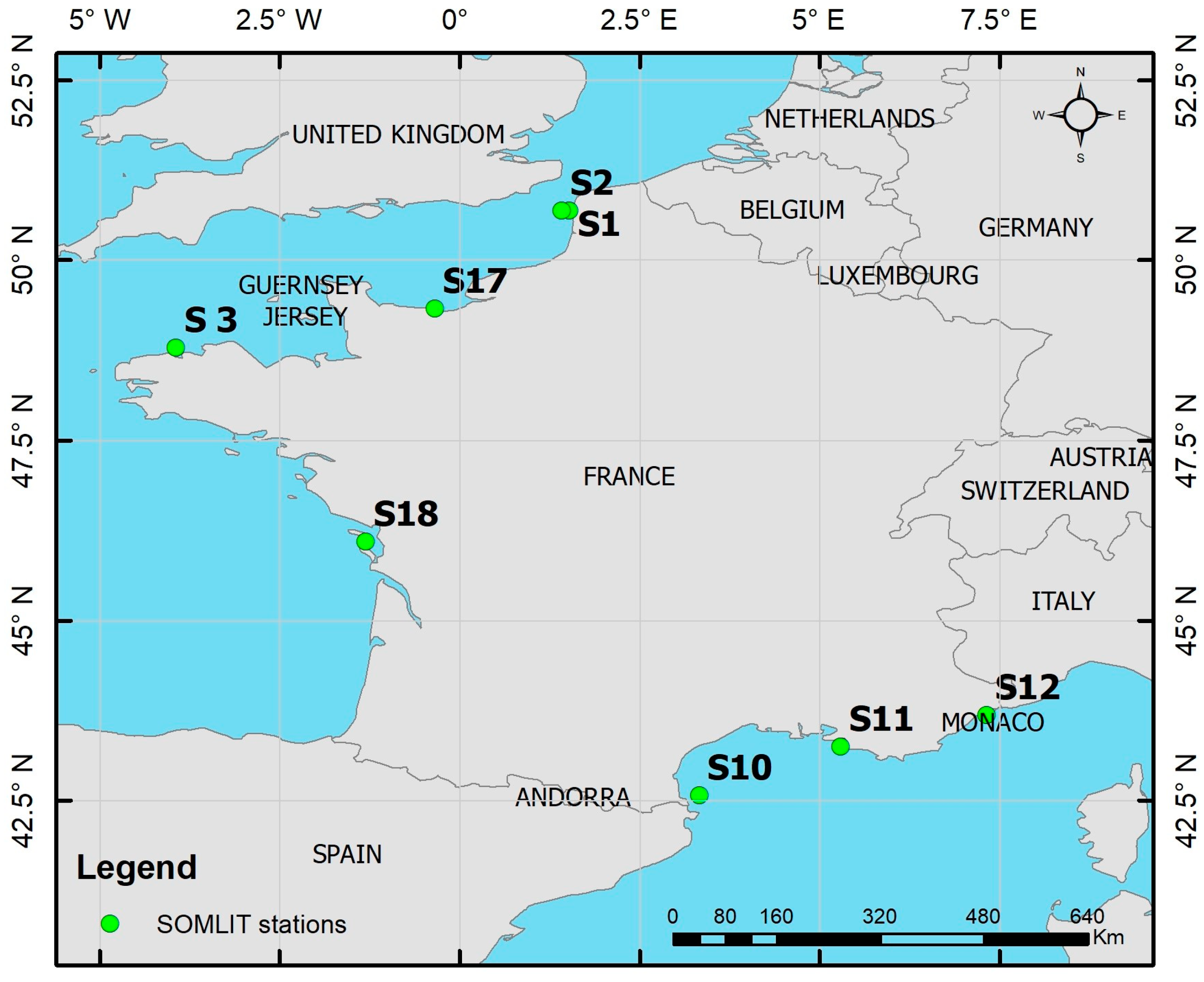
| S 01 | Wimereux, North of France (Channel Sea) | 1.6 | 30 | 6 |
| S 02 | Wimereux, North of France (Channel Sea) | 8.1 | 56 | 11 |
| S 03 | Roscoff, Brittany (Channel Sea) | 3.5 | 42 | 30 |
| S 10 | Banyuls-sur-Mer (Mediterranean Sea) | 0.8 | 92 | 78 |
| S 11 | Marseille (Mediterranean Sea) | 4.8–6.4 | 69 | 28 |
| S 12 | Villefranche-sur-Mer, French Riviera, (Mediterranean Sea) | 0.5 | 44 | |
| S 17 | Luc-sur-Mer, Normandy, (Channel Sea) | 0.175 | 1 | |
| S 18 | La Rochelle, Bay of Biscay (Atlantic Ocean) | 8.046 | 2 | 1 |
| Total | 336 | 154 |
| Authors | Abbreviation | Inputs | Region | POC Range (μg L−1) | N |
|---|---|---|---|---|---|
| Band ratio-based algorithms | |||||
| Stramski et al. 2008 | S08-1S08-2 | Rrs(443)/Rrs(555) Rrs(490)/Rrs(555) | Eastern South Pacific | 10–270 | 53 |
| Woźniak et al. 2016 | W16-1 W16-2 | Rrs(555)/Rrs(589), Rrs (490)/Rrs(625) | Baltic Sea Gulf of Gdańsk (Poland) | 145–2370 | 73 |
| Hu et al. 2015 | Hu15-1 Hu15-2 Hu15-3 | Rrs(443)/Rrs(555) Rrs(490)/Rrs(555) Rrs(510)/Rrs(555) | China Sea | 17.59–687.5 | 120 |
| Liu et al. 2015 | Liu15 | Rrs(678)/Rrs(488) & Rrs(748)/Rrs(412) | Pearl River Estuary, (China) | 113–1402 | 103 |
| Rrs based algorithm | |||||
| Le et al. 2016 | Le16-1 Le16-2 | Rrs(488), Rrs(532), Rrs(547), Rrs (667), Rrs(678) Rrs(490), Rrs(510), Rrs(550), Rrs (670) | Louisiana & Mobile Bay (Gulf of Mexico) | 11.5–230 | 230 |
| Color index algorithm | |||||
| Le et al. 2018 | Le18-1 Le18-2 | Rrs(490) & Rrs(555) & Rrs(665), Rrs(443)/Rrs(555) | Global ocean * | 52.6–375.2 | 297 |
| X | Functional Form | ao | a1 | a2 | R2 | RMSDlog |
|---|---|---|---|---|---|---|
| log(Rrs(665)/Rrs(555)) | Power | 3.097 | 1.122 | 0.59 | 0.267 | |
| log(Rrs(665)/Rrs(510)) | Power | 2.926 | 0.906 | 0.65 | 0.249 | |
| log(Rrs(665)/Rrs(490)) | Power | 2.861 | 0.833 | 0.66 | 0.246 | |
| log(MRB) | Power | 2.875 | 0.928 | 0.67 | 0.242 | |
| log(MRB) | Second-order polynomial | 2.873 | 0.945 | 0.025 | 0.67 | 0.242 |
| Algorithms | N | MAPD | MB | RMSDlog | RMSD | MR | R2 | Slope | Intercept | Negative Value |
|---|---|---|---|---|---|---|---|---|---|---|
| CPOC-1st | 195 | 38.37 | −2.77 | 0.25 | 488.02 | 1.03 | 0.60 | 0.78 | 0.58 | 0 |
| CPOC-2nd | 195 | 37.48 | 0.54 | 0.25 | 489.88 | 1.02 | 0.60 | 0.78 | 0.58 | 0 |
| Hu15-1 | 195 | 64.40 | 29.45 | 0.32 | 581.37 | 1.55 | 0.39 | 0.32 | 1.9 | 0 |
| Hu15-2 | 195 | 38.83 | −104.8 | 0.28 | 582.1 | 1.14 | 0.48 | 0.35 | 1.72 | 0 |
| Hu15-3 | 195 | 38.87 | −74.53 | 0.27 | 589.8 | 1.11 | 0.47 | 0.5 | 1.31 | 0 |
| Le16-1 | 195 | 61.75 | 127.5 | 0.38 | 943.3 | 1.52 | 0.22 | 0.4 | 1.7 | 0 |
| Le16-2 | 144 | 60.89 | 1237 | 0.44 | 4715 | 1.59 | 0.42 | 0.9 | 0.46 | 0 |
| Le18-1 | 195 | 1781 | 1,340,760 | 1.76 | 13,608,584 | 18.81 | 0.08 | 0.94 | 1.48 | 0 |
| Le18-2 | 195 | 68.94 | 157.7 | 0.35 | 651.5 | 1.63 | 0.39 | 0.48 | 1.52 | 0 |
| Liu15 | 134 | 62.71 | 202.8 | 0.38 | 749.4 | 1.4 | 0.28 | 0.62 | 1.1 | 10 |
| S08-1 | 195 | 45.09 | −60.53 | 0.3 | 584.0 | 1.26 | 0.39 | 0.36 | 1.73 | 0 |
| S08-2 | 195 | 49.19 | 44.14 | 0.29 | 590.4 | 1.41 | 0.48 | 0.47 | 1.51 | 0 |
| W16-1 | 150 | 64.29 | 214.9 | 0.44 | 842.5 | 1.04 | 0.48 | 1.13 | −0.33 | 0 |
| W16-2 | 146 | 61.32 | 247.5 | 0.34 | 715.1 | 1.48 | 0.53 | 0.91 | 0.35 | 0 |
| S08-1* | 193 | 45.46 | −61.03 | 0.30 | 587.0 | 1.26 | 0.38 | 0.35 | 1.75 | 0 |
| S08-2 * | 193 | 49.19 | 44.47 | 0.30 | 593.5 | 1.41 | 0.48 | 0.46 | 1.52 | 0 |
© 2019 by the authors. Licensee MDPI, Basel, Switzerland. This article is an open access article distributed under the terms and conditions of the Creative Commons Attribution (CC BY) license (http://creativecommons.org/licenses/by/4.0/).
Share and Cite
Tran, T.K.; Duforêt-Gaurier, L.; Vantrepotte, V.; Jorge, D.S.F.; Mériaux, X.; Cauvin, A.; Fanton d’Andon, O.; Loisel, H. Deriving Particulate Organic Carbon in Coastal Waters from Remote Sensing: Inter-Comparison Exercise and Development of a Maximum Band-Ratio Approach. Remote Sens. 2019, 11, 2849. https://doi.org/10.3390/rs11232849
Tran TK, Duforêt-Gaurier L, Vantrepotte V, Jorge DSF, Mériaux X, Cauvin A, Fanton d’Andon O, Loisel H. Deriving Particulate Organic Carbon in Coastal Waters from Remote Sensing: Inter-Comparison Exercise and Development of a Maximum Band-Ratio Approach. Remote Sensing. 2019; 11(23):2849. https://doi.org/10.3390/rs11232849
Chicago/Turabian StyleTran, Trung Kien, Lucile Duforêt-Gaurier, Vincent Vantrepotte, Daniel Schaffer Ferreira Jorge, Xavier Mériaux, Arnaud Cauvin, Odile Fanton d’Andon, and Hubert Loisel. 2019. "Deriving Particulate Organic Carbon in Coastal Waters from Remote Sensing: Inter-Comparison Exercise and Development of a Maximum Band-Ratio Approach" Remote Sensing 11, no. 23: 2849. https://doi.org/10.3390/rs11232849
APA StyleTran, T. K., Duforêt-Gaurier, L., Vantrepotte, V., Jorge, D. S. F., Mériaux, X., Cauvin, A., Fanton d’Andon, O., & Loisel, H. (2019). Deriving Particulate Organic Carbon in Coastal Waters from Remote Sensing: Inter-Comparison Exercise and Development of a Maximum Band-Ratio Approach. Remote Sensing, 11(23), 2849. https://doi.org/10.3390/rs11232849