Comparison of Lake Optical Water Types Derived from Sentinel-2 and Sentinel-3

Abstract

Inland waters play a critical role in our drinking water supply. Additionally, they are important providers of food and recreation possibilities. Inland waters are known to be optically complex and more diverse than marine or ocean waters. The optical properties of natural waters are influenced by three different and independent sources: phytoplankton, suspended matter, and colored dissolved organic matter. Thus, the remote sensing of these waters is more challenging. Different types of waters need different approaches to obtain correct water quality products; therefore, the first step in remote sensing of lakes should be the classification of the water types. The classification of optical water types (OWTs) is based on the differences in the reflectance spectra of the lake water. This classification groups lake and coastal waters into five optical classes: Clear, Moderate, Turbid, Very Turbid, and Brown. We studied the OWTs in three different Latvian lakes: Burtnieks, Lubans, and Razna, and in a large Estonian lake, Lake Võrtsjärv. The primary goal of this study was a comparison of two different Copernicus optical instrument data for optical classification in lakes: Ocean and Land Color Instrument (OLCI) on Sentinel-3 and Multispectral Instrument (MSI) on Sentinel-2. We found that both satellite OWT classifications in lakes were comparable (R² = 0.74). We were also able to study the spatial and temporal changes in the OWTs of the study lakes during 2017. The comparison between two satellites was carried out to understand if the classification of the OWTs with both satellites is compatible. Our results could give us not only a better overview of the changes in the lake water by studying the temporal and spatial variability of the OWTs, but also possibly better retrieval of Level 2 satellite products when using OWT guided approach.

1. Introduction

The remote sensing of inland waters is getting more attention, because traditional in-situ methods cannot monitor lakes with the temporal and spatial frequency demands in the European Union Water Framework Directive (WFD) [1]. Inland waters are known to be optically complex and more diverse than marine or ocean waters. Therefore, the remote sensing of these waters is more challenging. To obtain correct water quality products, the first step in remote sensing of lakes could be the classification of the water types because lake optical properties can vary in time and space, depending on the changes in weather, biological composition, and physical attributes. Thus, one method for all lakes or even in the same lake might not work well [2,3,4]. This approach has been practiced in sea water [5,6,7,8,9], and it is also a recent trend in inland waters [10,11,12,13,14,15,16].

Lakes can be categorized based on their richness in nutrients, which together with available light typically affect vegetation and phytoplankton growth [17]. In the case of a shallow lake, light reaches to the bottom and photosynthesis can occur in the entire water column. The nutrients (e.g., phosphate, nitrate, and sulphate) are used for growth. If the nutrients are in the dark, they cannot be used. Thus, in addition to the nutrient based classification, it is important to know the depth of the lake. Nutrient-poor lakes are considered as oligotrophic, and they generally have clear water, having a low concentration of phytoplankton. Mesotrophic lakes have good clarity and an average level of nutrients. Eutrophic lakes are rich with nutrients, resulting in high concentrations of phytoplankton and possible algal blooms. Lastly, a lake is considered hypertrophic if the water is excessively enriched with nutrients. Lakes typically reach this condition due to human activities, such as heavy use of fertilizers in the lake catchment area. Such lakes are of little use to humans and have a poor ecosystem due to decreased dissolved oxygen. Most oligotrophic lakes are deep and eutrophic lakes are typically shallow [17].

Lake optical properties can vary in time and space, depending on the changes in weather, biological composition, and physical attributes [18]. For lakes in the northern hemisphere, it is typical to have spring blooms after ice-melt and a rise in water temperature [17]. Warm summers cause even more intensive blooms that can last for weeks. Most often, not only the biomass of phytoplankton is changing, but also the composition of its dominant species. Sometimes toxic cyanobacteria can occur, which can be harmful to humans or other animals using the lake water. Cyanobacteria become dominant due to an ability to use nitrogen from the air when all nitrogen from the water has been used up. Hence, the detection of cyanobacteria blooms is gaining more importance [19].

Remote sensing of inland waters has specific requirements of satellite instrument spatial and spectral resolution [3]. For example, the spatial resolution must be high enough to exclude the coastal area of the lake, but due to often very irregular shapes of lakes, this can be challenging. Another very important aspect in optical water research is the existence of suitable bands. In the European Space Agency Earth Observation program Copernicus [20], among others, two different missions have launched that are suitable for the study of inland waters: Sentinel-2 [21,22,23,24] and Sentinel-3 missions [25].

The Sentinel-2 mission is a land monitoring constellation of two satellites (A and B, launched in 2015 and 2017, respectively) that are equipped with the state-of-the-art Multispectral Instrument (MSI), which offers high-resolution optical imagery: 10 m, 20 m, and 60 m spatial resolution, depending on the spectral band. MSI samples in 13 spectral bands. This mission provides global coverage of the Earth’s land surface every 10 days with one satellite and 5 days with 2 satellites, making the data of great use in on-going studies [26].

Sentinel-3 is primarily an ocean mission; however, the mission is also able to provide atmospheric and land applications. This is, similar to Sentinel-2, a constellation of two satellites (A and B, launched 2016 and 2018, respectively). Sentinel-3 is equipped with a medium resolution (300 m) Ocean and Land Color Instrument (OLCI) for marine research (21 spectral bands) that provides global coverage every two days [26].

Both satellites have their advantages and disadvantages for inland water monitoring. Sentinel-3 has been built to monitor waters, but its low spatial resolution limits the research to only the largest lakes. Although Sentinel-2 has suitable spatial resolution for inland waters, it lacks some of the bands of critical wavelengths that Sentinel-3 has, such as the chlorophyll-a (chl-a) absorption peak at 685 nm.

Compared with traditional in-situ monitoring methods, the use of satellite data gives advantages of good temporal coverage, spatial coverage over the entire lake, a large view over the region, and access to past conditions. Depending on the socio–economic importance of the given lake, traditional in-situ measurements can vary from once per month to once every five years, while remote sensing data can have up to a daily frequency. Spatial coverage can play an important role in determining the quality of the lake water in the entire lake, since just one or a couple of sample points might not describe the entire lake and can miss important bloom events in the lake.

The primary goal of this study was to investigate if Sentinel-2 and -3 give compatible results in determining the optical water types (OWTs). In the current work, the Uudeberg et al. [16] classification of OWTs was used because it was based on boreal region lakes, which corresponds to our study lakes. This classification has all the OWTs of this region, including brown waters, that might be missing in other similar classifications. Additionally, the aim was to discover the spatial and temporal differences of lake OWTs in Latvia and Estonia during 2017.

2. Materials and Methods

2.1. Study Sites

We studied four optically different northern-boreal lakes: three of them are in Latvia and one is in Estonia.

2.1.1. Lake Burtnieks

Lake Burtnieks, the fourth biggest lake (40.2 km²) in Latvia, is situated in the Northern part of Latvia, 47 m above sea level. The shallow (average depth 2.4 m, max depth 4.3 m) lake has an oval shape with a max width of 5.5 km. The banks are shallow and sandy, but along the southern coast, waves have carved sandstone cliffs [27]. According to the Latvian lake monitoring database, Lake Burtnieks is classified as a shallow brown water lake with high water hardness. Monitoring results from 2002 to 2017 [28] showed chl-a values in the range of 1.2–321.3 mg m^–3 with a median value of 32.3 mg m^–3. The transparency was measured with the Secchi disk in range of 0.2–2.1 m with a median value of 0.6 m.

2.1.2. Lake Lubans

Lake Lubans lies in the center of the Eastern Latvian Lowland. It is a shallow (average depth 1.6 m, max depth 3.5 m) drainage lake. After damaging spring floods in 1926, several dams and ditches were constructed. The elevation of the lake is allowed to fluctuate between approximately 90 and 93 m above sea level. At an elevation of 90.75 m, the lake has an area of 25 km², increasing to about 100 km² at 92.75 m. In that stage, it is considered to be the biggest lake in Latvia. Lake Lubans is surrounded by wetlands (area 813 km²). It is a unique natural formation of European and global importance with an important role in the preservation of many protected species and biotopes; 225 bird species have been recorded in the lake surroundings, of which 51 are enlisted among the most protected species in Latvia [27]. According to the Latvian lake monitoring database, Lake Lubans is classified as a very shallow clear water lake with high water hardness. Monitoring results from 2006 to 2014 [28] showed chl-a values in the range of 6.1–83.9 mg m^–3 with a median value of 18.4 mg m^–3. The transparency measured with the Secchi disk was in range of 0.4–1.6 m with a median value of 0.8 m.

2.1.3. Lake Razna

Lake Razna (57.6 km²) is often called the sea of Latgale (average depth 7 m, max depth 17 m). It is the second biggest lake in Latvia by area and largest by water volume (0.46 m³). Lake Razna is situated on the Raznava hill. The level of the water reaches 163.8 m above sea level. The lake is rich with 27 various fish species. Lake Razna is included in Razna National park (created in 2006), which is included in the European Union network of protected areas NATURA 2000 [27]. According to the Latvian lake monitoring database, Lake Razna is classified as a shallow clear water lake with high water hardness. Monitoring results from 2002 to 2017 [28] showed chl-a values in the range of 0.4–34.5 mg m^–3 with a median value of 2.6 mg m^–3. The transparency measured with the Secchi disk was in range of 1.7–9.0 m with a median value of 3.8 m.

2.1.4. Lake Võrtsjärv

Lake Võrtsjärv is a large lake (270 km², water volume 0.8 km³), and it is the second largest lake in Estonia. The shallow (average depth 2.7 m, max depth 6 m) lake is 33.7 m above sea level. Lake Võrtsjärv is considered a hard-water eutrophic lake [29]. Its water is optically turbid and the underwater light climate is very strongly affected by the lake’s water level and ice conditions [30]. Transparency measured with the Secchi disk is in the range of 0.3–1.6 m and chl-a varies from 20 to 102 mg m^–3 [31]. Its catchment area (3100 km²) makes up about 7% of Estonian territory and, thus, contributes significantly to the Estonian natural CO₂ budget. A specific feature of Lake Võrtsjärv is the large natural climate-related variability of the water level, which causes up to a 3-fold difference of its water volume [32].

2.2. Satellite Data

The cloud-free or partially cloud free MSI on Sentinel-2A (Sentinel-2) (10–60 m pixel size) Level 1 images were downloaded from Copernicus Open Access Hub [33]. OLCI on Sentinel-3A (Sentinel-3) full resolution (300 × 300 m pixel size) Level 1 images were downloaded from Copernicus Online Data Access [34]. Altogether, 152 cloud free Sentinel-3 scenes for the four lakes were processed for the ice-free period in 2017, and 45 cloud free Sentinel-2 scenes were found.

Pre-processing of the images was carried out with a scientific image processing toolbox called the Sentinel Application Platform (SNAP v 6.0) developed by Brockmann Consult, Array Systems Computing and C-S [35]. The processing of Sentinel-2 images contains four steps: resampling all bands to 20 m resolution; sub-setting the case study lake from the entire scene; applying the multi-sensor pixel identification tool (IdePix), which classifies each pixel as water or land, and cloud-free or not, and identifies the type of the clouds and determines the cloud shadows; the “clearwater” mask was used, where only water pixels are included, that do not have any type of cloud, cloud shadow or aquatic vegetation flags raised; and images were processed with the Case-2 Regional CoastColor (C2RCC) [36] processor for atmospheric correction and retrieval of water leaving reflectance spectra. C2RCC was suggested by Ansper and Alikas [22] who tested many different atmospheric correction processors. The temperature was modified according to the average water temperature in Estonian and Latvian Lakes (

Table 1. The water temperature (T) values used in processing of the Sentinel-2 and Sentinel-3 images with the Case-2 Regional CoastColor (C2RCC) atmospheric correction processor depending on the month.

Month	Mar	Apr	May	Jun	Jul	Aug	Sep	Oct	Nov
T in °C	4	7.5	15	17.5	20	20	15	7.5	4

). Salinity was set always to 0.1 PSU.

Sentinel-3 image processing involved three steps: sub-setting the image to the desired size; applying the IdePix tool and creating a “clear water mask”, because IdePix is not generating this automatically for Sentinel-3; in addition, opposite to Sentinel-2, IdePix tool do not have cirrus cloud or aquatic vegetation risk flagging for Sentinel-3, that should kept in mind to avoid false interpretations of the results; merging the IdePix flags onto the original Level 1 image, because with Sentinel-3 the IdePix product has no original radiance bands included; and applying the C2RCC processor for atmospheric correction and retrieval of reflectance spectra. The temperature was again modified according to the average water temperature in Estonian and Latvian Lakes (Table 1), and salinity was set always to 0.1 PSU.

2.3. Classification of Optical Water Type (OWT)

The method by Uudeberg et al. [16] was applied for classification of OWTs. It divides inland and coastal water of boreal region into five OWTs based on reflectance spectrum key features, such as spectra maximum location, slopes, and amplitude (Figure 1). Each OWT is linked with a specific bio-optical condition. Clear OWT is associated with the highest water transparency and the lowest optically active substance concentrations. In Moderate OWT, all these concentrations are higher, but none of them dominate. In Turbid OWT, the total suspended matter dominates and reflectance spectra have the highest values. In Very Turbid OWT, the chl-a dominates; this type is associated with blooms. In Brown OWT, the colored dissolved organic matter (CDOM) dominates, and waters are dark and reddish to brown.

The OWT classification was applied to each Sentinel-3 and Sentinel-2 satellite image pixel reflectance spectrum. The OWT for each reflectance spectra of the pixel of the satellite image was determined by the maximum likelihood of individual spectrum to OWT reference reflectance spectra, using spectral correlation similarity (SCS) and modified spectral angle similarity (MSAS). This was calculated by the equation 1 [16]:

$${\delta }_j=10\left(SCS+\frac{1-MSAS}{2}\right),$$

where j denotes the OWT, and SCS and MSAS are calculated according to Homayouni et al. [37]. The reflectance spectrum of satellite image pixel was classified into OWT, which has the highest δ value. The used method also pre-analyses images before applying the OWT classification. In case the reflectance spectrum of the pixel of the satellite image were strongly affected other sources than water, and reflectance spectra shape and values were abnormal in the blue part of spectra, then pixel was not included into the OWT classification process and pixel was marked as “Unclassified”.

3. Results and Discussion

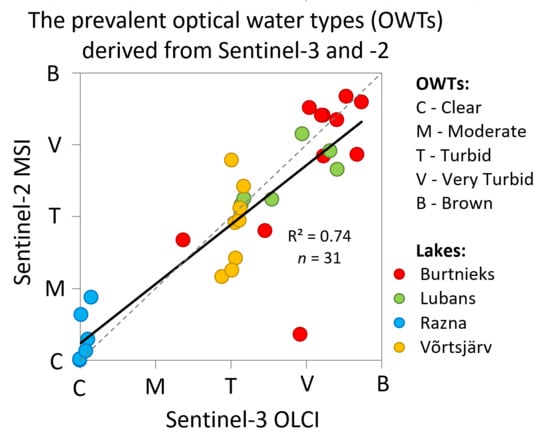
3.1. Comparison of the OWT Variability

Based on all the valid pixels of the cloud-free scenes of the lakes during 2017 (152 Sentinel-3 and 45 Sentinel-2 images), generally, the two instruments resulted in similar retrieval of OWTs. Brown OWT was dominating in Lake Burtnieks, which was also classified as shallow lake with brown water [28]. Turbid OWT was dominating in Lake Lubans and Lake Võrtsjärv, and Clear OWT in Lake Razna during 2017 (Figure 2). Except for the dominating OWTs, the two instruments gave different results. For example, in Lake Võrtsjärv with Sentinel-3, the majority of the pixels were determined as Turbid and only 9% were the other OWTs; but Sentinel-2 showed that 50% of the pixels were determined as other than Turbid OWT. Additionally, 92% of the Lake Razna Sentinel-3 pixels were determined as Clear OWT and this lake was classified as a shallow clear water lake [28]. In the case of Lake Lubans, the OWTs obtained varied from Turbid to Brown; however, it was classified as a very shallow clear water body [28]. Overall, Sentinel-2 data showed more variety in different OWTs, while Sentinel-3 tended to be homogenous in the OWTs, especially in lakes Razna and Võrtsjärv.

We found 31 cases with both Sentinel-2 and -3 cloud-free images from the lakes during 2017. This allowed us to compare the results of different instruments from the same day. The distribution of the OWTs of all the 31 matches showed that the best agreement between the two instruments was in Lake Razna and Lake Lubans (Figure 3), where the proportions of OWTs were similar to each other. The most disagreements seemed to be in Lake Võrtsjärv, where the differences between Sentinel-2 and -3 on the OWTs over the lake were remarkable on half of the matching days. Mostly, it seemed that in May and June, the Moderate OWT was dominating on Sentinel-2 data instead of Turbid, which was the absolutely dominating OWT in Lake Võrtsjärv according to Sentinel-3 (Figure 3).

Since derived OWTs are dependent on the shape of the reflectance spectra, atmospheric correction can cause differences in OWTs. Atmospheric correction over water bodies is challenging because waterbodies are dark, and about 90% of the signal received by the sensor is not affected by the water itself [4]. When working with optically complex waters, finding working atmospheric correction tool for the region is even more challenging, and often the result is over- or under-corrected [4]. For example, the shape of the reference reflectance spectrum of the Moderate and Turbid OWTs are quite similar, except the magnitude (Figure 1), so here over-or under-atmospheric correction have a definite impact to the retrieval of the OWTs. However, we used the same C2RCC processor for atmospheric correction for both instruments, but because of the differences in the band locations and the width of the bands itself, that can have an impact to the results, we still could not rule out that some of the differences were caused by the atmospheric correction processor itself. Since instruments have different spectral scales the OWT classification for Sentinel-2 is more sensitive to changes in input reflectance [16].

We compared the weighted prevalent OWT in the lakes for all the matching days between the two instruments. Each OWT was assigned by a number (Clear—1; Moderate—2, Turbid—3; Very Turbid—4, Brown—5). Then an average for all the lake pixels was found. In this way the correlation between the two instruments on the matching cases was better demonstrated (R² = 0.74) (Figure 4). It was seen that often the prevalent OWT agreed closely or was close to each neighboring OWT (Clear and Moderate, or Moderate and Turbid); furthermore, in natural water, the optical properties were continuous and there were always points between the two classes. In Lake Razna, the agreement on the prevalent OWT between the two satellites was the highest: 83% of the prevalent OWT was the same (Clear OWT). In Lake Võrtsjärv, the agreement was somewhat lower: 62.5% (Turbid OWT). In Lake Lubans the agreement was 50% on Turbid OWT and in Lake Burtnieks the satellites agreed on 45.5% of the match-up cases (mostly on Very Turbid OWT). The disagreement on the prevalent OWT was the strongest in Lake Burtnieks, where, for example, Sentinel-3 showed Very Turbid or Brown OWT, yet at the same time Sentinel-2 showed Clear OWT. Especially noticeable is an “outlier” of Lake Burtnieks from 12 May 2017, where the differences of the derived OWTs were quite extreme (Figure 3 and Figure 4), without this date the correlation was noticeably improved (R² = 0.87, n = 30). The misclassification of the OWTs came from the very different shapes of the reflectance spectra. In the case of very brown waters, the atmospheric correction might be problematic by strongly overestimating the blue part of the reflectance spectrum [16]. In Lake Lubans, the difference of the prevalent OWT was either Turbid or Brown (Figure 3 and Figure 4).

To study the impact of the spatial resolution differences in the satellite data, we resampled the 31 matching Sentinel-2 scenes to the Sentinel-3 spatial resolution (300 m). The prevalent OWT remained same, except in one case (Lake Lubans, 27 Sept 2017: Turbid to Very Turbid) where the difference between Turbid and Very Turbid were already quite equal for the 20 m resolution Sentinel-2 data (Figure 3). The average change between OWTs derived from high- and low-resolution Sentinel-2 data was 4.4%: Clear 2.8%; Moderate 4.5%; Turbid 7.1%; Very Turbid 4.4%; Brown 5.5%; and Unclassified 2.1%. Resampling to lower resolution had the overall largest impact to the Turbid OWT and the smallest to the Clear OWT. The standard deviation of the change remained generally around 7%. The median of the change over the 31 cases was quite low for each OWT (0-2.2%), except for Turbid OWT (7.1%). The resampling seemed to have also some impact on the spatial variability of the OWTs; this is quite expected and confirms the usefulness of the high spatial resolution of the remote sensing data. When comparing the new resampled Sentinel-2 results to the Sentinel-3, then the relationship between the Sentinel-3 and Sentinel-2 resampled prevalent OWTs was weaker, where R² drops from 0.74 to 0.67. Also, all the correlations and standard errors of the OWTs separately were weaker with resampled Sentinel-2 data.

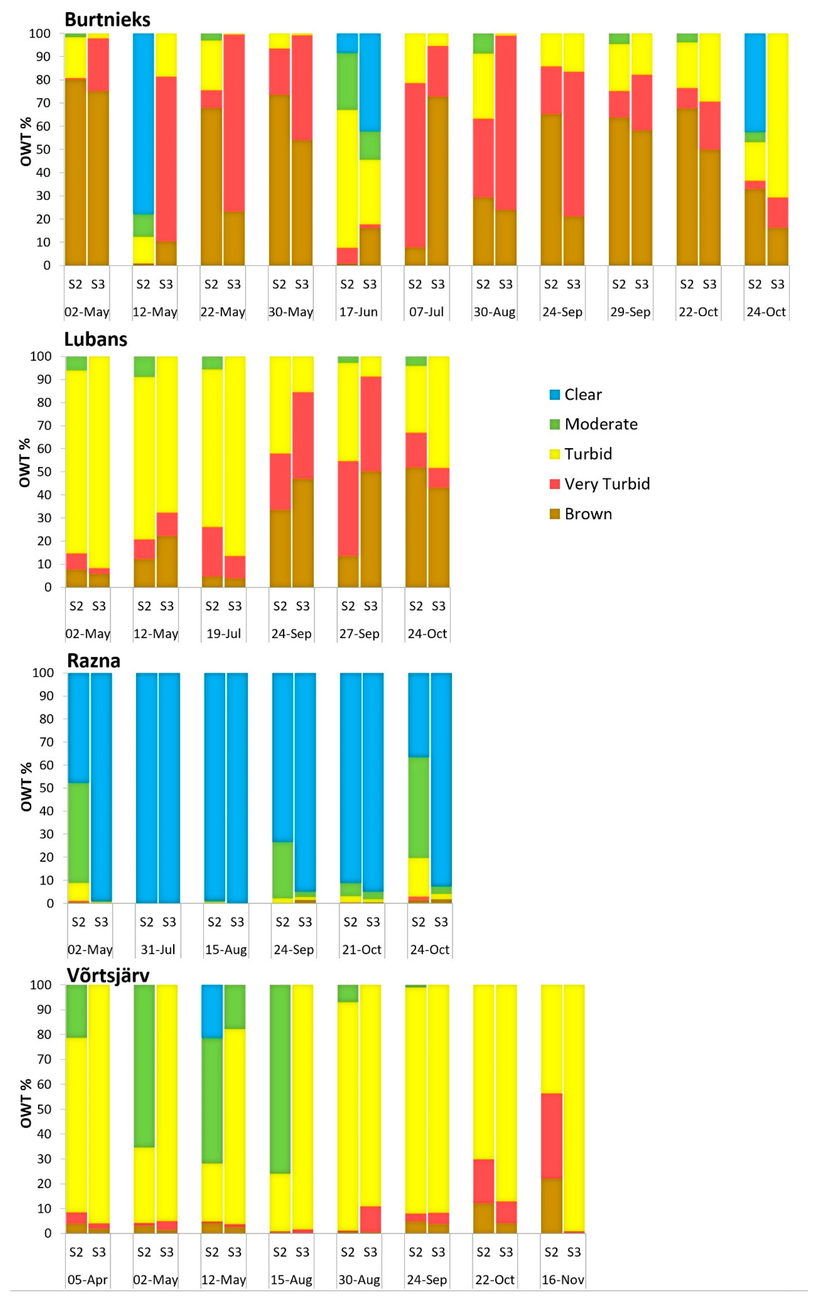
3.2. Spatial Variability

The Sentinel-2 and -3 images also made it possible to see the spatial variations of the OWTs in each study lake, which is one of the advantages that remote sensing data gives over in-situ monitoring. As said above, there were altogether 31 matching cases between Sentinel-2 and -3 cloud-free images from which we could compare the spatial differences in OWT classification. We have displayed four of them in Figure 5.

Although in some cases spatial variability is seen from Sentinel-3 images (Lake Burtnieks and Lake Lubans in Figure 5), Sentinel-2 with higher spatial resolution is able to monitor smaller lakes and finer patterns. This is a strong advantage in vegetation rich lakes, where Sentinel-2 can detect OWTs in clear water between the patches of vegetation, whilst Sentinel-3 pixels are affected with vegetation and are not good for monitoring the quality of the water. Generally, in Lake Burtnieks both instruments agreed on the spatial variability of the OWTs, but quite often disagreed on the OWT itself, for example Very Turbid and Brown OWTs (Figure 3 and Figure 5). The reasons behind this could be related to the difficulties of the atmospheric correction in brown waters, as discussed above. Lake Burtnieks often showed great spatial variability of OWT, because the naturally quite brown water lake could often have heavy blooms [38]. In the case of Lake Lubans, mostly it was seen that the coastal areas were more Turbid or Brown OWTs. As said in the previous section, Lake Võrtsjärv showed very homogeneous water according to the Sentinel-3 data. Additionally, the literature described a lake as having homogenous waters where a single measurement point of a lake describes 90% of the lake [39]. However, with Sentinel-2, there were fine patterns of different OWTs shown. Typically, the narrow south part was Very Turbid and Brown, and the northern bigger part was Moderate and Turbid with some Very Turbid mixed in. This agrees with the characteristics of the lake bottom: the southern part of the lake bottom is organic rich mud while the northern part is sandy [40]. The most agreement between both satellites was found in Lake Razna, because it is a deep and clear water lake, although in some cases, Sentinel-2 detected more Moderate OWT pixels in the lake than Sentinel-3, especially in the coastal zone.

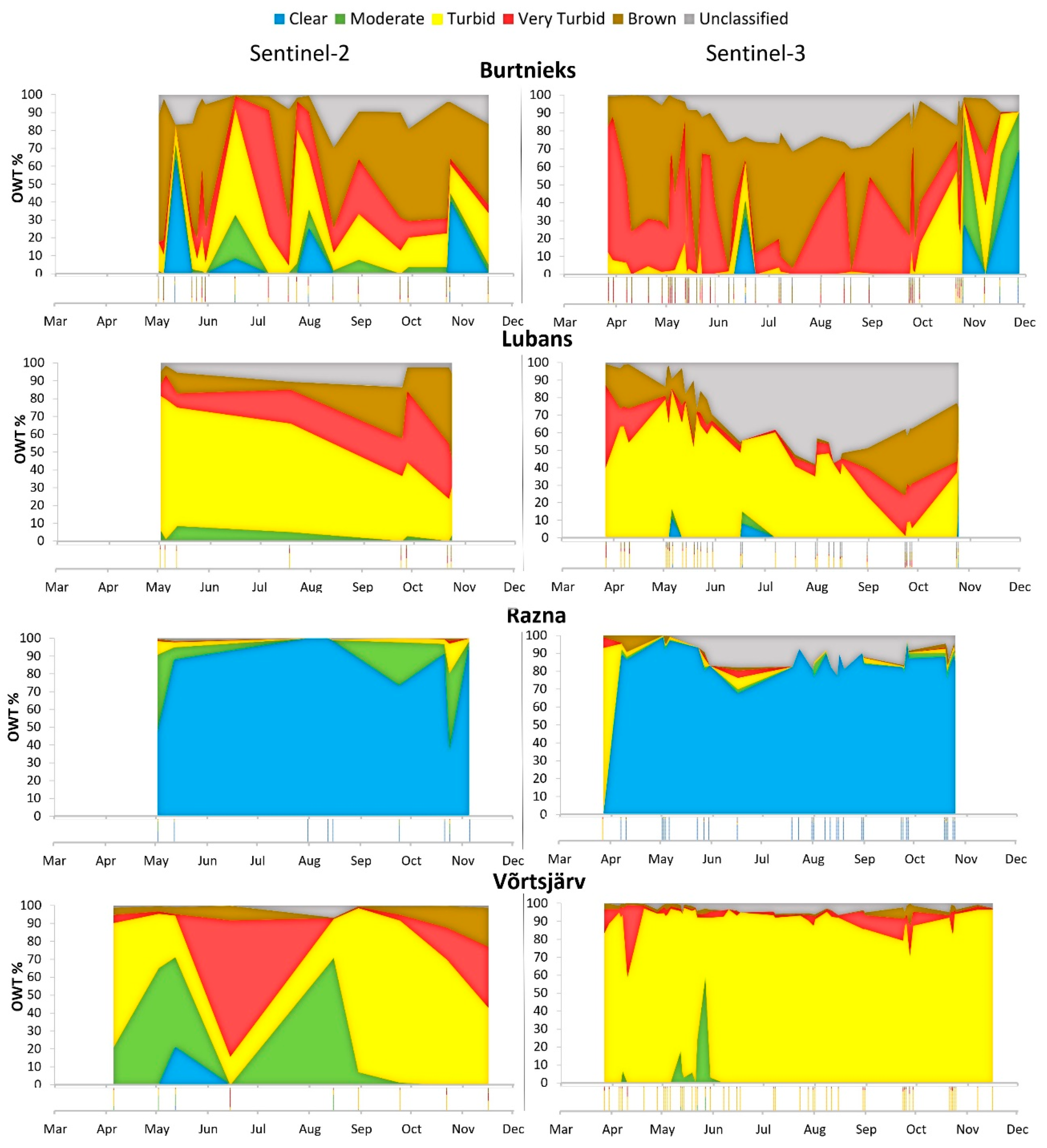
3.3. Temporal Variability

Temporal variability shows a change in the lake optical properties during different seasons. Here, one ice-free period was studied, from early spring to late autumn of 2017 (Figure 6). Lake Burtnieks seemed to be in a favorable location for Sentinel-2; it was seen from three tiles, so there was more coverage than on the other lakes (19 days, while the others had 8 or 9 days). In Lake Burtnieks, the OWTs changed quite rapidly from Brown to Very Turbid OWT or vice versa (Figure 6). That was most likely due to fluctuations in chl-a concentrations. The rapid changes could also be caused by the combination of water level fluxes and intensive agriculture [38]. Additionally, dry or rainy summers might influence the water level and the water quality of the inflows, but some part may be due to the above discussed OWT classification sensitivity of reflectance spectra changes and the influence of atmospheric correction. Thus, here it would be beneficial to carry out in-situ measurements for further validation of the results in order to evaluate the factors of atmospheric correction that could cause or causes the disturbances in OWT classification.

The other three lakes showed more stability in their temporal variability in the OWTs. Lake Lubans and Lake Razna showed approximately similar pattern in the OWTs. The influence of infrequent data was shown most clearly on Lake Võrtsjärv, where the overall temporal variability was affected by one June Sentinel-2 image (prevalently Very Turbid OWT while Sentinel-3 had mostly Turbid OWT) (Figure 6). Here, we have to take into account that with Sentinel-3 we had 47 scenes from Lake Võrtsjärv over 2017, and with Sentinel-2 we had only 9 scenes; therefore, one day had more proportional weight with Sentinel-2. Additionally, the more data we had from different days per year, the better overview we had on the temporal variability; therefore, less than 10 images per year made the temporal variability analysis of OWTs from Sentinel-2 quite unreliable (Figure 6). The fewer images there were for the temporal analysis of the OWTs, the more weight every single image had, although, with in-situ measurements, we often made conclusions on the water condition with even lower temporal resolution. From over 2000 Latvian lakes, only a small part of them are monitored monthly, and less than 300 lakes have just one sampling during a 3-year period [41]. In Estonia, from over 2300 lakes, only Lake Võrtsjärv is monitored monthly. Twelve other lakes are monitored up to five times per year. There are 90 other lakes that are monitored up to twice over a five-year period [42].

The other difference in the Sentinel-2 and -3 OWT data was the quantity of the “unclassified” pixels. In total, about 10% of Sentinel-3 clear water pixels and only 3% of Sentinel-2 pixels were “unclassified”. Those were inland water pixels with strong influences from land or in-water vegetation in their reflectance spectra. Typically, the increase in the “unclassified” share in Sentinel-3 OWT data during summer describes the influences from the coast, including the coastal vegetation. This was especially clearly seen in Lake Lubans (Figure 6). At the same time, this effect was not seen in Sentinel-2 data. The number of Sentinel-2 pixels used for OWT classification assignments per lake decreased during the summer. For example, in Lake Lubans and Lake Burtnieks, the decrease of the “clear water” pixels was significant (44% and 54%, respectively). In Lake Razna the decrease of suitable pixels was 24% and in Lake Võrtsjärv it was 12%. This was because in the pre-processing, the IdePix tool was working well on Sentinel-2 images. Not only did it identify the cirrus and other translucent clouds, but it also distinguished the vegetation dominated pixels. Therefore, the number of “unclassified” pixels was rather low with Sentinel-2 (

Table 2. The percentages of the derived optical water types (OWTs) from Sentinel-2 (S2) and Sentinel-3 (S3). The number (No.) of scenes and pixels denote the total number of images and pixels used. The most abundant OWT percentage is shown with bold for each lake.

Lake	Burtnieks		Lubans		Razna		Võrtsjärv
Satellite	S2	S3	S2	S3	S2	S3	S2	S3
No. of scenes	19	42	8	32	9	31	9	47
No. of pixels	1,478,576	17,521	1,463,540	33,519	1,179,890	18,701	4,972,075	132,849
Clear %	8.1	3.7	0	1.3	80.1	83.7	2.0	0.1
Moderate %	4.1	2.3	3.4	1.5	15.0	1.5	22.9	2.8
Turbid %	19.6	10.0	50.8	46.7	4.0	3.5	49.5	88.5
Very Turbid %	14.5	31.5	19.0	8.9	0.3	0.4	17.3	4.1
Brown %	44.0	41.0	21.2	13.6	0.4	1.5	7.0	1.9
Unclassified %	9.6	11.5	5.6	28.0	0.3	9.4	1.3	2.7

). Since Sentinel-3 can fail in clear water identification, the derived Level 2 products (for example chl-a) from coastal areas should be taken with extra caution, even when no quality flags are raised.

4. Conclusions

From previous studies it is clear that in the estimation of inland water quality products, the first step should be OWT classification [4,15,16]. In this study, a comparison of OWTs between Sentinel-2 and -3 was carried out. Generally, both instruments gave compatible results. Additionally, we studied the spatial and temporal differences of lake OWTs in Latvia and Estonia during 2017.

There are lakes with quite strong dominance for certain OWT (Lake Võrtsjärv and Lake Razna) and those whose dominant OWTs change often (Lake Burtnieks). The cause for the rapid changes in the dominant OWT in Lake Burtnieks might be the changing water quality. Lake Lubans has mostly Turbid OWT, opposite to clear waters according to the current Latvian classification [28], and the lake loses a large amount of the water surface to the developing coastal vegetation during the summer (the “unclassified” pixels).

The results between the two satellite instruments generally agreed on the dominant OWT in a lake. The differences might be caused by several factors: the atmospheric correction processor used (C2RCC); the differences in the spatial resolution of the two instruments; and the sensitivity of the OWT model to the slightly different reflectance spectra of the two sensors, due to the different spectral bands.

Unfortunately, the moderately low spatial resolution of Sentinel-3 limits the research to only larger lakes in Latvia and Estonia. Additionally, the finer details on the spatial variability of the OWT is lost in smaller lakes. Sentinel-2A and B can now provide nearly the same data acquisition frequency, and their much higher spatial resolution can allow assessment of practically all lakes (including all lakes requested by the WFD).

OWT classification is already a data product that can be used for the cross-checking of lake water type classes. This supports our understanding of the spatial and temporal variability of the water quality; therefore, it provides useful knowledge in planning the frequency of in-situ monitoring and the locations of the sampling stations. OWTs in lakes allows us to monitor the long-term changes and it is also an excellent platform to create different algorithms in optically complex waters on the basis of OWT.

References

1. The European Parliament; The Council of the European Union. WFD Directive 2000/60/EC of the European Parliament and of the Council of 23 October 2000 establishing a framework for Community action in the field of water policy. Off. J. Eur. Parliam. 2000, 372, 275–346. [Google Scholar]
2. Bukata, R.P. Retrospection and introspection on remote sensing of inland water quality: Like déjà vu all over again. J. Great Lakes Res. 2013, 39, 2–5. [Google Scholar] [CrossRef]
3. Palmer, S.C.J.; Kutser, T.; Hunter, P.D. Remote sensing of inland waters: Challenges, progress and future directions. Remote Sens. Environ. 2015, 157, 1–8. [Google Scholar] [CrossRef] [Green Version]
4. Matthews, M.W.; Bernard, S.; Lain, L.R.; Griffith, D.; Odermatt, D.; Kutser, T. Understanding the Satellite Signal from Inland and Coastal Waters. In Earth Observations in Support of Global Water Quality Monitoring; IOCCG Report Series, No. 17; Greb, S., Dekker, A., Binding, C., Eds.; International Ocean Color Coordinating Group: Dartmouth, NS, Canada, 2018; pp. 55–68. [Google Scholar]
5. Morel, A.; Prieur, L. Analysis of variations in ocean color. Limnol. Oceanogr. 1977, 22, 709–722. [Google Scholar] [CrossRef]
6. Baker, K.S.; Smith, R.C. Bio-optical classification and model of natural waters. Limnol. Oceanogr. 1982, 27, 500–509. [Google Scholar] [CrossRef]
7. Moore, T.S.; Campbell, J.W.; Dowell, M.D. A class-based approach to characterizing and mapping the uncertainty of the MODIS ocean chlorophyll product. Remote Sens. Environ. 2009, 113, 2424–2430. [Google Scholar] [CrossRef]
8. Moore, T.S.; Dowell, M.D.; Bradt, S.; Ruiz-Verdú, A. An optical water type framework for selecting and blending retrievals from bio-optical algorithms in lakes and coastal waters. Remote Sens. Environ. 2014, 143, 97–111. [Google Scholar] [CrossRef] [Green Version]
9. Melin, F.; Vantrepotte, V. How optically diverse is the coastal ocean? Remote Sens. Environ. 2015, 160, 235–251. [Google Scholar] [CrossRef]
10. Reinart, A.; Herlevi, A.; Arst, H.; Sipelgas, L. Preliminary optical classification of lakes and coastal waters in Estonia and South-Finland. J. Sea Res. 2003, 49, 357–366. [Google Scholar] [CrossRef]
11. Le, C.; Li, Y.; Zha, Y.; Sun, D.; Huang, C.; Zhang, H. Remote estimation of chlorophyll a in optically complex waters based on optical classification. Remote Sens. Environ. 2011, 115, 725–737. [Google Scholar] [CrossRef]
12. Shi, K.; Li, Y.; Zhang, Y.; Li, L.; Lv, H.; Song, K. Classification of inland waters based on bio-optical properties. J. Sel. Top. Appl. Earth Observ. Remote Sens. 2014, 7, 543–561. [Google Scholar] [CrossRef]
13. Shen, Q.; Li, J.; Zhang, F.; Sun, X.; Li, J.; Li, W.; Zhang, B. Classification of several optically complex waters in China using in situ remote sensing reflectance. Remote Sens. 2015, 7, 429–440. [Google Scholar] [CrossRef] [Green Version]
14. Eleveld, M.A.; Ana, B.; Ruescas, A.B.; Hommersom, A.; Moore, T.S.; Peters, S.W.M.; Brockmann, C. An Optical Classification Tool for Global Lake Waters. Remote Sens. 2017, 9, 420. [Google Scholar] [CrossRef] [Green Version]
15. Spyrakos, E.; O’Donnell, R.; Hunter, P.; Miller, C.; Scott, M.; Simis, S.; Neil, C.; Barbosa, C.; Binding, C.; Bradt, S.; et al. Optical types of inland and coastal waters. Limnol. Oceanogr. 2018, 63, 846–870. [Google Scholar] [CrossRef] [Green Version]
16. Uudeberg, K.; Ansko, I.; Põru, G.; Ansper, A.; Reinart, A. Using Optical Water Types to Monitor Changes in Optically Complex Inland and Coastal Waters. Remote Sens. 2019, 11, 2297. [Google Scholar] [CrossRef] [Green Version]
17. Wetzel, R.G. Limnology. Lake and River Ecosystems, 3rd ed.; Academic Press: Cambridge, MA, USA, 2001. [Google Scholar]
18. Ogashawara, I.; Mishra, D.R.; Gitelson, A.A. Remote Sensing of Inland Waters: Background and Current State-of-the-Art. In Bio-Optical Modeling and Remote Sensing of Inland Waters; Mishra, D.R., Ogashawara, I., Gitelson, A.A., Eds.; Elsevier Inc.: Amsterdam, The Netherlands, 2017; pp. 1–24. [Google Scholar]
19. Dörnhöfer, K.; Oppelt, N. Remote sensing for lake research and monitoring-recent advances. Ecol. Indic. 2016, 64, 105–122. [Google Scholar] [CrossRef]
20. Copernicus. Available online: http://www.copernicus.eu (accessed on 11 October 2019).
21. Toming, K.; Kutser, T.; Laas, A.; Sepp, M.; Paavel, B.; Nõges, T. First Experiences in Mapping Lake Water Quality Parameters with Sentinel-2 MSI Imagery. Remote Sens. 2016, 8, 640. [Google Scholar] [CrossRef] [Green Version]
22. Ansper, A.; Alikas, K. Retrieval of Chlorophyll a from Sentinel-2 MSI Data for the European Union Water Framework Directive Reporting Purposes. Remote Sens. 2019, 11, 64. [Google Scholar] [CrossRef] [Green Version]
23. Molkov, A.A.; Fedorov, S.V.; Pelevin, V.V.; Korchemkina, E.N. Regional Models for High-Resolution Retrieval of Chlorophyll a and TSM Concentrations in the Gorky Reservoir by Sentinel-2 Imagery. Remote Sens. 2019, 11, 1215. [Google Scholar] [CrossRef] [Green Version]
24. Zeng, C.; Binding, C. The Effect of Mineral Sediments on Satellite Chlorophyll-a Retrievals from Line-Height Algorithms Using Red and Near-Infrared Bands. Remote Sens. 2019, 11, 2306. [Google Scholar] [CrossRef] [Green Version]
25. GLaSS Deliverable D5.5: Boreal Lakes Case Study Results. Available online: http://www.glass-project.eu/assets/Deliverables/GLaSS-D5.5-Final.pdf (accessed on 1 August 2019).
26. ESA Earth Online. Available online: earth.esa.int/web/guest/missions/esa-eo-missions (accessed on 8 October 2019).
27. Ezeri.lv. Available online: http://www.ezeri.lv (accessed on 5 February 2019).
28. LEGMC (State Limited Liability Company “Latvian Environment, Geology and Meteorology Centre”) National Monitoring Database. Available online: http://www.meteo.lv/lapas/noverojumi/virszemes-udens/virszemes-udens_ievads?id=1369&nid=477 (accessed on 8 March 2018).
29. Mäemets, A. Eesti NSV Järved ja Nende Kaitse; Valgus: Tallinn, Estonia, 1977. [Google Scholar]
30. Reinart, A.; Nõges, P. Light conditions in Lake Võrtsjärv. In Lake Võrtsjärv; Haberman, J., Pihu, E., Raukas, A., Eds.; Estonian Encyclopedia Publishers: Tallinn, Estonia, 2004; pp. 141–149. [Google Scholar]
31. Paavel, B.; Arst, H.; Reinart, A. Variability of bio-optical parameters in two North-European large lakes. Hydrobiologia 2008, 599, 201–211. [Google Scholar] [CrossRef]
32. Nõges, T.; Nõges, P.; Laugaste, R. Water level as the mediator between climate change and phytoplankton composition in a large shallow temperate lake. Hydrobiologia 2003, 506, 257–263. [Google Scholar] [CrossRef]
33. Copernicus Open Access Hub. Available online: scihub.copernicus.eu (accessed on 17 February 2018).
34. Copernicus Online Data Access. Available online: coda.eumetsat.int (accessed on 17 February 2018).
35. Zuhlke, M.; Fomferra, N.; Brockmann, C.; Peters, M.; Veci, L.; Malik, J.; Regner, P. SNAP (sentinel application platform) and the ESA sentinel 3 toolbox. In Proceedings of the Sentinel-3 for Science Workshop, Venice, Italy, 2–5 June 2015; Volume 734. [Google Scholar]
36. Brockmann, C.; Doerffer, R.; Peters, M.; Kerstin, S.; Embacher, S.; Ruescas, A. Evolution of the C2RCC neural network for Sentinel 2 and 3 for the retrieval of ocean colour products in normal and extreme optically complex waters. In Proceedings of the Living Planet Symposium, Prague, Czech Republic, 9–13 May 2016; Volume 740, p. 54. [Google Scholar]
37. Homayouni, S.; Roux, M. Hyperspectral image analysis for material mapping using spectral matching. Int. Arch. Photogramm. Remote Sens. Spat. Inf. Sci. 2004, 35, 49–54. [Google Scholar]
38. Bilaletdin, Ä.; Frisk, T.; Kaipainen, H. An integrated modelling system for the water protection project of Lake Burtnieks. Int. Ver. Theor. Angew. Limnol. Verhandl. 2006, 29, 1399–1403. [Google Scholar] [CrossRef]
39. Nõges, P.; Tuvikene, L. Spatial and annual variability of environmental and phytoplankton indicators in Lake Võrtsjärv: Implications for water quality monitoring. Estonian J. Ecol. 2012, 61, 227–246. [Google Scholar] [CrossRef] [Green Version]
40. Raukas, A. Bottom deposits. In Lake Võrtsjärv; Haberman, J., Pihu, E., Raukas, A., Eds.; Estonian Encyclopedia Publishers: Tallinn, Estonia, 2004; pp. 79–86. [Google Scholar]
41. LEGMC (State Limited Liability Company “Latvian Environment, Geology and Meteorology Centre”), Assessment on Data Availability and Quality. Available online: www.meteo.lv/fs/CKFinderJava/userfiles/files/Par_centru/ES_projekti/Projekts_Udens_kvalitate/Assessment_on_data_availability_and_quality.doc (accessed on 9 October 2019).
42. Keskkonnaministeerium (Ministry of the Environment), Water Monitoring Program 2016–2021. Available online: http://www.envir.ee/et/eesmargid-tegevused/vesi/vesikondade-veeseireprogramm-2016-2021 (accessed on 14 October 2019).
Figure 1. The reference reflectance spectra used for each optical water type (OWT) [16].
Remotesensing 11 02883 g001
Figure 2. The proportion of the optical water types (OWTs) ("unclassified" pixels excluded, included in Table 2) in 2017 from all cloud-free images in different lakes.
Remotesensing 11 02883 g002
Figure 3. The distribution of the optical water types (OWTs) for all Sentinel-2 and -3 matching cases.
Remotesensing 11 02883 g003
Figure 4. Correlation between the prevalent optical water type (OWT) derived from Sentinel-3 and -2 images. Colors represent different lakes: blue—Razna; green— Lubans; yellow— Võrtsjärv; red— Burtnieks. The x-and y-axes represent the OWTs: 1—Clear; 2—Moderate; 3—Turbid; 4—Very Turbid; 5—Brown.
Remotesensing 11 02883 g004
Figure 5. The comparison of the spatial variability of the optical water types (OWTs) between Sentinel-2 and -3 in four different lakes at selected dates. The upper row for each lake shows the enhanced red, green, blue (RGB) images, the second shows the spatial variability of the OWTs, and the third row shows the percentages of each OWT of the given scene.
Remotesensing 11 02883 g005
Figure 6. Temporal variability and the distribution of the optical water types (OWTs) derived from Sentinel-2 and Sentinel-3 in different lakes during 2017. The lower panel of each sub-figure shows the frequency of the acquired data.
Remotesensing 11 02883 g006