Article

Assessment of the Biomass Productivity Decline in the Lower Mekong Basin

1
Soils and Fertilizers Research Institute (SFRI), Duc Thang, Bac Tu Liem, 11910 Hanoi, Vietnam
2
Department of Engineering Systems and Environment, University of Virginia Charlottesville VA 22904, USA
3
Hydrological Sciences Lab, NASA Goddard Space Flight Center, Greenbelt, MD 20771, USA
*
Author to whom correspondence should be addressed.
Remote Sens. 2019, 11(23), 2796; https://doi.org/10.3390/rs11232796
Submission received: 3 October 2019 / Revised: 30 October 2019 / Accepted: 22 November 2019 / Published: 26 November 2019
(This article belongs to the Special Issue Monitoring Vegetation Phenology: Trends and Anomalies)

Abstract

:
This study aimed to delineate the geographic hotspots of negative trends in biomass productivity in the Lower Mekong Basin countries (Vietnam, Cambodia, Laos, and Thailand) and identify correlated regional environmental and anthropogenic factors. A long-term time-series (1982–2015) of Normalized Difference Vegetation Index at a resolution of approximately 9.16 km × 9.16 km was used to specify the areas with significant decline or increase in productivity. The relationships between vegetation changes and land attributes, such as climate, population density, soil/terrain conditions, and land-cover types, were examined. Rainfall time-series maps were used to identify areas that might have been affected by land degradation from those correlated with rainfall. Most of the detected potentially degraded areas were found in Cambodia, the Northwest and the Highland of Vietnam, the Northern Mountains of Thailand and Laos, and the mountainous border between Laos, Vietnam, and Cambodia. About 15% of the total land area of these four countries experienced a reduction in biomass productivity during the 34-year study period. The map of hotspots of changes in productivity can be used to direct further studies, including those at finer spatial resolution that may support policy makers and researchers in targeting the strategies for combating land degradation.

Graphical Abstract

1. Introduction

In addition to climate change and biodiversity loss, land degradation is considered a significant and far-reaching global problem [1,2,3,4,5,6,7,8]. Land degradation threatens global development goals, especially those related to global food security and poverty reduction [9,10]. In the tropical countries, where livelihoods are often agriculture-based, land degradation is a serious problem for food security and development of society [11,12,13,14]. Tropical countries tend to harbor areas where land degradation and climate change have severe environmental and socioeconomic impacts [15].
Land is defined as a combination of terrestrial ecosystem that includes soil resources, vegetation, water, other biotas, landscape setting, climate attributes, and ecological processes. Land degradation is defined as “the temporary or permanent decline in the productive capacity of the land” [16]. The phenomenon of land degradation, therefore, includes the degradation of vegetation functions and services, usually over time, either within a land-use/cover type (e.g., forest degradation and yield-degraded cropland), or a conversion of natural productive land-cover type to a less productive one (e.g., deforestation) [14], often including soil degradation. It has been measured through a loss of biomass, a loss of actual or potential productivity, or a loss or change in vegetative cover and soil nutrients. Soil and vegetation degradation are often linked. Land degradation is caused by both natural and anthropogenic factors [2,12,17,18]. Typical examples of natural causes of land degradation are frequent or prolonged droughts, or high rainfall on sloping land. Anthropogenic causes of land degradation are more complex, including a hierarchy of intermediate causes (e.g., deforestation, overgrazing, shifting cultivation with shortened fallow periods, and unbalanced fertilizer use) and underlying causes (e.g., population pressure, unsuitable land tenure regime, and poverty) [2,19,20]. Although anthropogenic (or human-induced) land degradation can be theoretically mitigated, it is a difficult task [21,22].
The Lower Mekong Basin (LMB) countries in this study include Cambodia, Laos, Thailand, and Vietnam (Figure 1). The livelihoods of millions of people (specifically in the Lower Mekong countries) rely strongly on agricultural production [23], and about 22% of the GDP is based on agriculture [24,25]. Recently, high population growth, the development of the economies, and modernization–urbanization have created an increased need for land for agricultural production [26]. A significant issue for the development is land degradation caused by deforestation, unsuitable land use, and inappropriate land management [27]. Land plays an important role in the livelihood in this region, but agricultural land per capita is low, and arable land has been rapidly decreasing [28].
In the 1990s, the scope of land-degradation research relied on soil-degradation assessment. The Assessment of the Status of Human-Induced Soil Degradation in South and South East Asia (ASSOD) [29] can be considered a first attempt to map soil degradation in the region, even though it has been shown to have significant limitations [30,31]. The limitations are as follow: (i) It was based only on soil degradation, and it ignored the decline of the other important components of the land, such as vegetation and biodiversity; (ii) The expert-based assessment could not be used in periodic quantitative monitoring over time; and (iii) Assessments were not spatially explicit [32]. Shrestha and Roy [33] assessed land degradation for the Greater Mekong sub-region by using various remote-sensing-derived indicators to combine into a composite land-degradation status. The results indicated that there were large portions of land areas severely degraded in LMB countries (10.7% total land in Cambodia, 18.2% in Laos, 18.7% in Thailand, and 17.9% in Vietnam). However, this assessment yielded the spatial data of degradation for the LMB countries at a specific time instead of showing the changes over long periods.
Information on the hotspots of land degradation is important for policy makers and researchers to combat land degradation on a regional and national level. The areas of severe degradation could help policy makers in prioritizing limited budgets and planning strategic interventions [32,34]. At national and regional scales, the main requirement is a view of areas where degradation magnitude and extent are relatively high for prioritizing the investments on the restoration or reclamation of degraded land, and focused field-based studies. With the geographic hotspot approach, the expected output is the map of degradation hotspots that can be seen as the first version of land degradation map to guide acquisition of the more comprehensive and accurate data in the next series of steps. However, the approach using the temporal states of soil parameters for assessment at large-scale is constrained by the lack of soil data for long-term quantitative comparisons [7]. On a continental or even a regional scale, it is impossible to develop time-series of soil properties that could detect persistent changes in soil status [12]. With the support of available satellite-driven time-series of global vegetation data that extends to more than 30 years in the past, an alternative approach applying the evaluation of changes in vegetation greenness or net primary productivity (NPP) has been applied [12,35,36,37,38]. Maps of land degradation have been developed at different scales, ranging from local, subnational, country, regional, and global scales, using vegetation indices from satellite observation [39]. Recently, the Normalized Difference Vegetation Index (NDVI), a relative measure of greenness and photosynthetic process, has a strong relationship with NPP, serving as an indicator of NPP and being used as a proxy for long-term biomass productivity decline or improvement [14,34,40,41,42,43,44,45,46]. The NDVI [47,48,49], which was derived from the Advanced Very High Resolution Radiometer (AVHRR) of the National Oceanic and Atmospheric Administration (NOAA) satellite, is used widely in the assessment of global or regional vegetation dynamics over a long duration (i.e., more than three decades) [50,51,52,53,54], and it can be combined with other data on climate, topography, soil, land use, and human demographics, to allow spatially explicit interpretation and analysis of the underlying processes of degradation [12,14,55]. Some previous studies [12,56,57,58] found that the human intervention or rainfall variations had varying effects on aboveground NPP in most biomes/climate zones. Previous studies showed that aboveground net primary production (represented by NDVI) has been shown to increase with increasing annual precipitation [12,57,59], and, indeed, correlation studies between rainfall and NDVI have been used to differentiate between human-induced and climate-induced land degradation [42,45,60,61], where any NDVI trends not explained by rainfall dynamics are ascribed to human actions. Topography affects climatic conditions [62,63,64], environment [65], and determines landscape and soil patterns [66,67,68,69], and thus affects vegetation cover [70,71]. Soil quality and primary productivity of standing vegetation have close interlinkages [7]. Thus, the distribution of the hotspots of land degradation in different soil and terrain conditions can provide some understanding of the processes that are involved [12]. Land use and vegetation cover is one important indicator of land degradation [33].
Though the approach based on NDVI time-series for detecting land degradation at a larger scale has been used in many studies, continuous verification in different geographic regions has been recommended [32]. For LMB countries, only a single study by Vu et al. [14] assessed land degradation for Vietnam, using spatiotemporal trend analysis, and found several hotspots of land degradation that could support policy makers and researchers in targeting the strategies for combating land degradation. The current study adopted the results from the abovementioned study and expanded it to the regional scale of several of the LMB countries. This study aimed to do the following: (i) Delineate the map of land degradation for the Lower Mekong River Basin countries (i.e., Vietnam, Laos, Cambodia, and Thailand) over the last three decades, and (ii) Identify the potentially underlying processes of the attributes of land (i.e., population density, soil/terrain conditions, and land use/land cover) that affect land degradation. The results of this study may help researchers and policy makers identify the locations where more detailed actions to prevent land degradation may be required.
In our approach, the decline of long-term trend NDVI was considered as proxy of NPP of the land, thereby representing past land-degradation hotspots. The decline of NDVI trend may include not only permanent degradation but also temporary degradation that can recover. It means the reduction of NDVI may simply be within the resilience of the vegetation, which enables it to recover from disturbance or stress (e.g., drought and floods) when the stressful conditions are removed [17]. Since we considered land degradation as the long-term reduction in the productive capacity of the land, both permanent and temporary degradation were taken into account in our study.

2. Materials and Methods

2.1. Study Area

The study area is characterized by a complex physical geography but can basically be separated into two main geographical zones. The first zone is dominated by low, flat topography in river valleys and deltas where paddy rice has been cultivated for centuries. The second zone consists of the plateaus and high mountainous areas dominated by high forest cover and shifting agriculture. The climate is governed by monsoon climate systems, with the southwest monsoon from May to late September and the northeast monsoon from November to early March. The annual precipitation ranges from 1000 to 3000 mm, and the mean temperature is around 24 °C, dependent on topography. The total population of the four LMB countries in 2017 was nearly 186 million, of which rural population was 60% (FAOSTAT, http://www.fao.org/faostat/). The total land area is around 1,262,190 km2, with the total agricultural area being 421,120 km2, and the arable land being 291,330 km2.

2.2. Datasets and Data Processing

The data used in this study were downloaded from different sources with different spatial resolutions (Table 1).
Since the data used in this study were downloaded from different sources with different spatial resolutions and types, they were processed to match the same resolution of GIMMS NDVI data (i.e., 1/12 degree or approximately 9.16 km resolution). We applied resampling methods depending on the data type. To preserve original data values and preserve the spatial consistency, resampling from coarse to fine resolution was carried out, using the nearest neighbor technique. To resample continuous datasets from fine to coarser resolution, the bilinear technique was applied. For categorical data, the resampling method, using the nearest neighbor technique, was carried out [81]. The spatial analyses in this study were carried out in Geographic Information System (GIS) environment, using ArcGIS software.

2.3. Methods

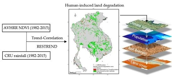
2.3.1. Proxy for Long-Term Biomass Productivity Decline at the Lower Mekong Basin Region

Long-term trend of NDVI recently used as a proxy for persistent decline or improvement in NPP of the land, thereby reflecting land degradation [12,34,35,42,43,44,45,60,82]. We applied this approach by using the NDVI derived from AVHRR satellite images, over the period 1982–2015. We aggregated the original GIMMS NDVI time-series (1/12 degree or 9.16 km pixel size, biweekly, period 1982–2015) to obtain the time-series of annual mean values as 12-month averages for interannual NDVI trend analysis. In applying the satellite-derived NDVI to assess biomass productivity, several issues regarding the NDVI-vegetation productivity relationship needed to be considered (i.e., cloud-cover effects, seasonal variations, and time-series autocorrelation). To avoid the effect of cloud cover or cloud shade in the humid tropic, only nonflagged pixels (i.e., flag = 0 indicates a good value of NDVI) were used. The problems of seasonal variations in vegetation phenology (direct proportion to weather seasonality) and time-series autocorrelation were minimized by using annual average NDVI and focusing on the declining “hotspots” where the interannual NDVI trend is most remarkable (i.e., with a statistical significance at the level of 90% (p < 0.1), which is sufficient for long-term trend analyses of noisy parameters like NDVI and the absolute trend magnitude greater than 10% of the beginning year over 34 years [12,34]. The recent findings of de Jong et al. [83,84] supported above treatment since they recognized that differences between the linear trends of annually aggregated GIMMS NDVI and the seasonal, nonparametric trends of the original GIMMS NDVI time-series (biweekly) were mainly on areas with weak or nonsignificant NDVI trends, which are not central in our hotspot approach.
To check whether the temporal trend of interannual NDVI could be credibly used as a proxy of temporal NPP trend, we compared the spatial pattern of GIMMS NDVI trend with MODIS NPP extracted from Terra MODIS Net Primary Production Yearly L4 Global 1 km (MOD17A3) V055 data product. The MODIS NPP data were resampled by using the bilinear technique from 1 to 9.16 km resolution. Two evaluation tests were carried out for overlaid time (2000–2014): (i) evaluation of the overlap area between the NDVI and NPP trends across the LMB countries and (ii) calculation of temporal correlation between interannual mean NDVI and NPP for each degraded pixel over the test period.
To compare GIMMS NDVI with MODIS NDVI, as suggested by Yengoh et al. [85], we extracted NDVI data from the Terra MODIS Vegetation Indices Monthly L3 Global 1 km (MOD13A3) V006, and then calculated the annual mean values as 12-month averages for the period 2001–2015. The data were resampled by using the bilinear technique to match the resolution of 9.16 km; thus, we applied the same evaluation tests as described in the above paragraph, but for GIMMS NDVI and MODIS NDVI datasets in the overlap period (2001–2015).

2.3.2. Pixel-Based Temporal Trend of Biomass Productivity

To identify the direction of vegetation variation (decrease or increase) over time, the NDVI time series was then statistically analyzed by using the linear regression of the period of 1982–2015. The trend of biomass productivity for each pixel, i, can be assessed by the slope coefficient (Ai) in the simple linear regression relationship:
Vi = Ai × t + Bi
where Vi = annual mean NDVI, Ai = long-term trend of NDVI, t = year (count from 1982 to 2015), and Bi = intercept (an indicator for a possible delay in the onset of degradation). The computed slope coefficient A for each pixel was tested for statistical significance at the level of 90% (p < 0.1).
A significant decline of the annual mean NDVI was determined when a pixel had (1) a negative NDVI slope (Ai < 0) with a statistical significance (p < 0.1) and (2) meaningful magnitude of the NDVI decline (relative NDVI annual reduction ≥10%/34 years [12,34].

2.3.3. Isolation of Rainfall Impacts

The stepwise analyses were used to find the areas where land productivity dynamics are highly correlated with rainfall change. NDVI trends in these areas can be explained by rainfall dynamics, and the remaining areas are most likely due to human actions. Rainfall data were obtained from the website of the Climatic Research Unit (CRU) [75]. The original data include grids of monthly rainfall and temperature data at a spatial resolution of 0.5° in the 1901–2015 period. Annual rainfall values for the period 1982–2015 were computed as 12-month averages. To isolate the impacts of rainfall, we applied two methods, the trend-correlation stepwise [12,34] (Trend-Correlation) and residual trend analysis [42,45,60] (RESTREND). For details of each method, readers are referred to Vu et al. [14]. Though the main limitation of the RESTREND method is that precipitation is considered as the unique driver of vegetation productivity in the analysis [50], the RESTREND method with the precipitation-alone technique was applied in the present study because the method has been most widely used for assessing the long-term changes in vegetation over the last few decades [42,45,59], and in the terrestrial ecosystems in tropics precipitation, it is still considered to be one of the main factors controlling the net primary production (NPP) [86]. Pixels with urban and industrial areas, based on the land-cover map from the SERVIR Mekong, were excluded from all spatial analyses. For Trend-Correlation method, if the pixel had a significantly negative NDVI trend (negative Ai, p < 0.1) and a strongly positive vegetation–rainfall correlation (R2 > 0.5; R > 0; p < 0.05), we concluded that the NDVI decline at the location was mainly determined by the rainfall factor. Otherwise, the NDVI decline could have been caused by human activities. For the RESTREND method, the NDVI was regressed from annual precipitation, and then the residuals—the difference between observed NDVI and NDVI as predicted from precipitation—were calculated (Figure 2). If there is a significant temporal trend of residual, then the declining biomass production may have been caused by factors other than a decline in precipitation. This method and other ones were well discussed in Rishmawi and Prince [87].
Results of the land-degradation areas delineated by both methods were compared. We merged the degraded areas by both methods to have the final land-degradation areas, as each method may be able to identify some degraded areas that may not successfully be detected by the other [14].

2.3.4. Relational Analyses of Potential Underlying Processes

In order to understand the relationship of land degradation and potential causes, the LMB countries in this study were divided into 3 major climate zones based on the Köppen–Geiger climate map [76]: tropical monsoon (Am), tropical savanna (Aw), and humid subtropical (Cwa). The climate zones of LMB were overlaid with the land-degradation map to obtain a map of degradation in climate zones.
First, to determine the relationship between population and land degradation, the mean population densities of each pixel were calculated by averaging 2000, 2005, 2010, and 2015 data. The mean population densities were overlaid with the map of degradation in climate zones, and then they were classified into three levels, as low density (less than the mean), very high density (greater than twice the mean), and high density (between the above two), as suggested by Vlek [12]. Those classes were used to differentiate the degraded pixels of the respective climate zones.
Second, land degradation in different climate zones was associated with soil and terrain conditions. We differentiated between the areas of land degradation by the topographic and soil-based suitability of the land for agriculture by using FAO and United States Geological Survey (USGS) databases. The terrain and soil constraints were considered with respect to agriculture production in all areas of LMB region. Soil-constraint classes were derived from the FAO-IIASA Global Agroecological Assessment for Agriculture [80] dataset by aggregation as follows: No/slight constraint (FAO class 1, 2, 3), Moderate constraint (FAO class 4 or 5), and Severe/Very severe constraint (FAO class 6, 7, or 8) (Table S1 in Supplementary Materials). Terrain constraints (i.e., slope and elevation) were extracted from SRTM (Shuttle Radar Topography Mission) elevation data. The three classes of terrain constraints were classified: No/slight constraint (0° ≤ slope ≤ 15° and elevation ≤ 3500 m above sea level—a.s.l.), Moderate constraint (15° < slope ≤ 25° and elevation ≤ 3,500 m a.s.l.), and Severe/Very severe constraint (slope > 25° or elevation > 3,500 m a.s.l.). The combinations of soil and terrain constraints are shown in Supplementary Materials (Table S2).
Land and vegetation cover is one important indicator of land degradation [33]. To examine the regions affected by land-degradation processes under different land-cover types, the land-cover map in 2015 were taken into account for analyses. As resolution of this regional study (i.e., 9.16 km pixel) and the patchy land-cover patterns in the region, some classes of land cover from SERVIR Mekong were combined, we used 6 land-cover types (i.e., mangrove, deciduous forest, evergreen broadleaf, mixed evergreen and deciduous, cropland, and others) for interpreting the hotspots of land degradation (Table S3 in Supplementary Materials).

3. Results

3.1. Proxy for Long-Term Biomass Productivity Decline

Our evaluation indicated consistency between the temporal dynamics of GIMMS NDVI and MODIS NPP. During the period 2000–2014, about 54% of the land area exhibited consistency in the direction between NDVI and NPP (increase of both NDVI and NPP or decrease of both NDVI and NPP) (Figure 3a). About 77% of the land area showed a positive correlation between interannual mean NDVI and NPPs (Figure 3b).
Figure 4 shows the results of evaluation tests between GIMMS NDVI and Terra MODIS NDVI for the period of 2001–2015. The results showed that, during the period 2000–2015, about 71% of the land area exhibited consistency in the direction between GIMMS NDVI and MODIS NDVI (increase of both datasets or decrease of both datasets). The statistics of the results from the map of the correlation coefficient (Figure 4b) indicate that about 91% of the land area exhibited a positive correlation between interannual mean GIMMS NDVI and MODIS NDVI. These results indicated good consistency between the temporal and spatial changes of GIMMS NDVI and MODIS NDVI datasets.

3.2. Temporal Trend of Biomass Productivity

The areas of significant improvements in biomass productivity were mainly found in the Red River Delta and Mekong River Delta of Vietnam, and the central plain and plateaus (Thailand) (Figure 5) consisting of 49% (629,368 km2) of total land of four countries. The areas that have experienced long-term biomass decline over the last 34 years were distributed in many areas of Cambodia; the Northwest, the Mekong Delta, and the Highland of Vietnam; the Northern Mountains of Thailand and Laos; and the mountainous shared border between Laos, Vietnam, and Cambodia (Figure 5). These areas occupied about 15% (186,298 km2) of total land of four countries. Differences between the area from FAO statistics in Methods, Section 2.3, and the area calculated from the maps shown in Results, Section 3, are due to the edge errors.

3.3. Isolation of Rainfall Variation Effect

To isolate the biomass productivity decline from the annual precipitation-driven signals over the last decades, we examined the correlation between green productivity (NDVI) and rainfall across LMB over the 35-year period. The Pearson’s correlation coefficient (R) for the period 1982–2015 for each pixel was measured to find the relationship between interannual NDVI and rainfall dynamics (Figure 6a). The results showed that the correlation coefficient ranged from +0.72 to –0.68. The regions where vegetation correlated positively with rainfall changes from year to year (the red colors in Figure 6a) covered mainly the flat area in Thailand and the Central Highland and Mekong River in Vietnam. The blue areas showed the negative correlation between NDVI and rainfall were located mainly in the border area shared by Vietnam, Laos, and Cambodia, and the North of Laos and Thailand. The correlation coefficient of every pixel was tested for statistical significances at the level of 95% (p < 0.05). Most of the degraded area showed the neutral correlation (i.e., –0.5 < R < 0.5 and/or not significant at p < 0.05), indicating that almost all degraded areas across the LMB countries have not been associated significantly with interannual variations in rainfall.
We isolated the degraded regions where rainfall has had a dominant impact on vegetation productivity from areas of degradation by applying the Trend-Correlation and RESTREND methods. A comparison of the results obtained from using the two methods is shown in Figure 6b. The areas of biomass productivity decline by the Trend-Correlation and RESTREND methods are 2,217 and 2,075 pixels, respectively. The degraded area shared by both methods is very high (i.e., 174,300 km2 or 94% of the total degraded area), demonstrating a high confidence level for the used methodology. Merging the results from both methods yielded the area of 186,228 km2 (15% of the total land area of four countries) that has been degraded after eliminating rainfall-driven pixels.
The results of the nationwide analyses of land degradation show that Cambodia had the highest rate of land degradation (32.6% of total national landmass). The percentage of land degradation in Vietnam was also high (about 16.9% of total national landmass), but it was lower than the result found in the previous study (i.e., 19%) [14]. The spatial distribution of degraded areas in Vietnam was found mainly in the Northwest, the Mekong River Delta, the Central Highland, and the Southeast, which were comparable with four priority regions mentioned in the National Action Programme to Combat Desertification for the Period 2006–2010 and the Orientation to 2020 (NAP 2006), and the same with results found by Vu et al. [14]. Laos and Thailand had the lowest rate of land degradation, about 13.7% and 7.4%, respectively. The rate of land degradation found in our study could not be compared directly to previous studies because of the differences in approach, datasets, and variables for assessment. However, if doing a comparison with results found by Shrestha and Roy [33], our assessment shows a bit lower proportion for Laos and Thailand, in line for Vietnam, but higher rate for Cambodia (Table 2).

3.4. Relational Analyses of Potential Underlying Processes

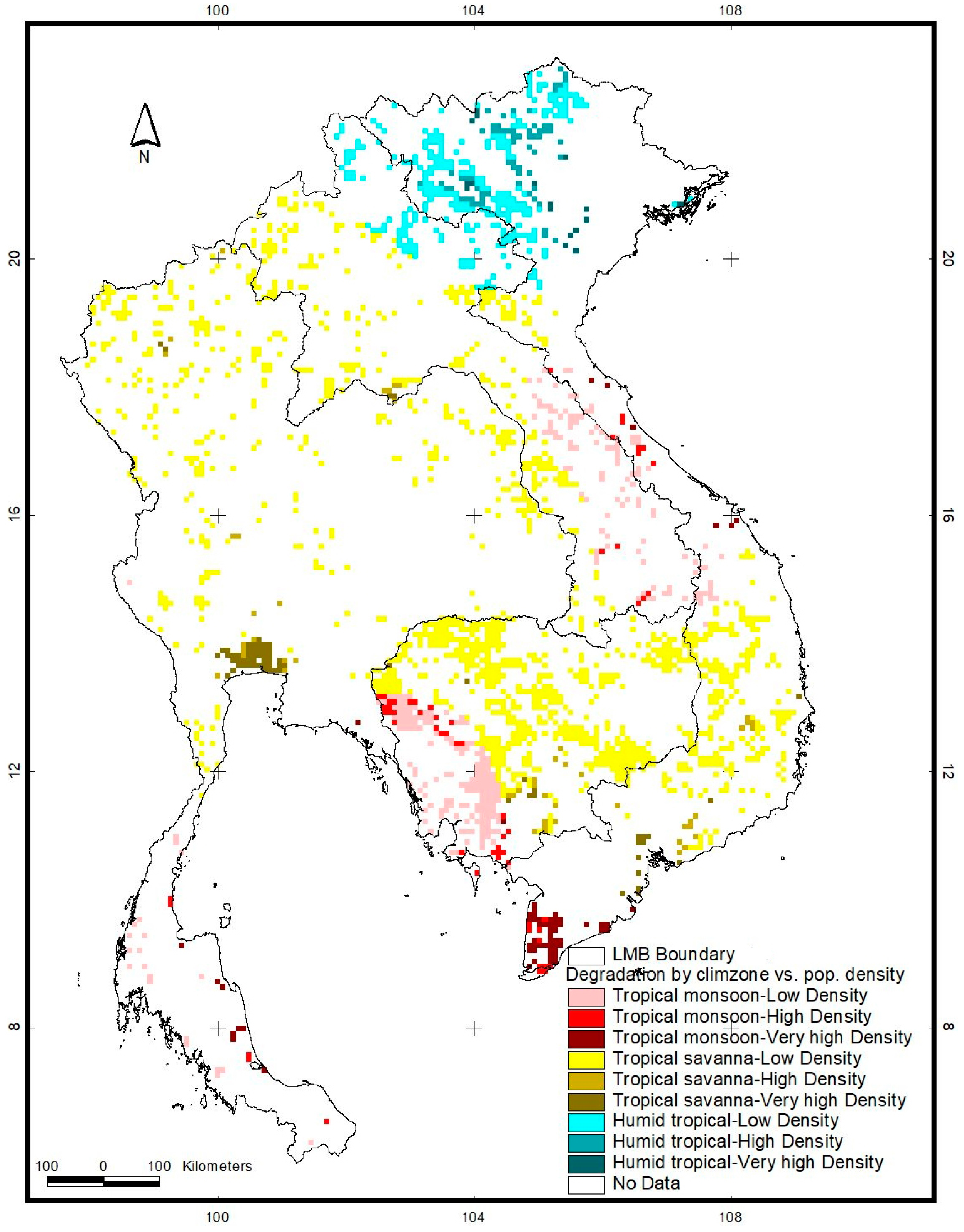
3.4.1. Climate Zones

Results from overlaying the climate zone map with land degradation showed that 64% of degraded area belonged to tropical savanna, including nearly the entirety of Thailand and Cambodia, as well as half of Laos and Vietnam. There were 19% of degraded area located in tropical monsoon, which cover mainly the middle part of Vietnam, the south of Laos, and some parts in the south of Thailand and Cambodia. The remaining area (17%) situated in humid subtropical covering almost the North of Vietnam and a small area of the Northeast of Laos.

3.4.2. Land Degradation in Relation to Population Density

When overlaying population density of the period 2000–2015 with the degraded area, the mean population densities were 110, 253, and 105 persons km−2 for the tropical monsoon, tropical savanna, and humid subtropical, respectively. Three classes of each climate zones were then created (i.e., low density, high density, and very high density) and used to differentiate the degrading pixels of the respective climate zones. Figure 7 shows the land degradation in different climate zones in relation to population density. Most of the land-degradation areas were located in places with a low population density (Table 3). Only some areas in the Mekong River Delta, the cities in the Northwest of Vietnam, and the areas near Bangkok, Thailand, show the land degradation with high population.

3.4.3. Land Degradation in Relation to Soil and Terrain Constraints and Population Densities

The result of the land-degradation areas classified by terrain and soil suitability for agriculture is shown in Figure 8 and Table 3. The areas that are severe/very severe constraints for agriculture comprise about 20,580 km2, or 11% of the total degraded area. Most of these pixels were found in regions with relatively low population density in the tropical savanna and humid tropical regions (Table 3). Only in the tropical monsoon-prone regions of Vietnam and Thailand were the degraded pixels with very severe soil/terrain constraint located in the very high population densities. The moderate soil/terrain constraint covered the largest area of land degradation (112.476 km2 or 62%). Similar to severe/very severe constraint, most of these pixels were found in regions with a low population density. The areas of no/slight soil/terrain constraint included about 275% total degraded area and were found mainly in tropical savanna and monsoon zones, and only 3% of this type of constraint was located in places with a very high population density.

3.4.4. Land Cover and Land Degradation Processes

Table 4 shows the area of the regions affected by land degradation processes under different land-cover types. The area of cropland that degraded is 65,352 km2 (36% total degraded area). Of the 20,664 km2 that are not suitable for agriculture (i.e., severe/very severe soil/terrain constraint in Table 4), 8988 km2 are actually being farmed (cropland). These regions were found mainly in the Central Highland (Vietnam), the Northwest (Cambodia), and near Bangkok (Thailand) (Figure 8). The remaining 56,364 km2 of cropland belonged to the areas that are suitable for agriculture (no/slight or moderate soil/terrain constraint). Mangrove is dominated in the tropical monsoon, so it is the most affected in this climate zone (about 70%). In the tropical savanna, different forest cover types are the most affected because they are predominant there (61,992 km2), of which about 6000 km2 are not suitable for agriculture and suffering by degradation processes. There are many areas of degradation which have agricultural potential but are used mainly for the forest (Figure 8).

4. Discussion

4.1. New Methods

This study presented an NDVI-based biomass productivity degradation assessment by using a multi-aspect approach. First, we checked whether interannual GIMMS NDVI trends could indicate the temporal trend of NPP. Many previous studies by Herrmann et al. [60], Helldén and Tottrup [82], and Vlek et al. [12], which assessed biomass productivity degradation by using NDVI time-series, supposed a strongly positive relationship between NDVI and NPP trends, without validating. We found that the land area with a positive correlation between the annual mean NDVI and NPPs was about 77%. Vu et al. [14] identified the correlation between the temporal dynamics of GIMMS NDVI and MOD17 NPP in the period of 2000–2006 for Vietnam and also found about 75% of the NDVI declining area showed a positive correlation. The findings also agree with other previous studies [40,88,89] and confirm that the AVHRR-NDVI trend can be used as a proxy for land productivity. In our study, the consistency between the spatial patterns of interannual trends of the two variables was evaluated as suggested by Wessels [90], instead of analyzing the relationship between mean annual NDVI and NPP through space.
Second, we evaluated the consistency between GIMMS NDVI and MODIS NDVI datasets. A number of studies evaluating the consistency between above datasets [91,92] concluded that both the datasets agreed well, but should be confirmed in future assessments of vegetation activities [93]. Using MODIS NDVI as a benchmark of GIMMS NDVI, as suggested by Yengoh et al. [85], we found consistency between temporal and spatial changes of GIMMS and MODIS NDVI datasets over the period of 2001–2015. The findings were similar to another study by Tucker et al. [94]. The study carried out by Gallo et al. [93] also showed that there was a strong correlation (R > 0.9) when comparing AVHRR and MODIS NDVIs for different land-cover types. Du et al. [95] found that about 82% of Qing-Hai-Tibet Plateau area was characterized by a strong consistency between GIMMS and MODIS NDVI at the pixel scale. Fensholt [96] assessed the accuracy of GIMMS by using MODIS NDVI (2000–2010), which indicated that overall trends of GIMMS and MODIS NDVIs were in acceptable agreement. Our findings agreed with those assessments and indicated that GIMMS NDVI could be used as a proxy indicator for biomass productivity analyses in the next steps.
Third, we examined ‘convergent validity’, to isolate declining biomass productivity from the climate-driven signals. According to Scholz and Tietje [97], convergent validity can be established if two different methods to evaluate the same issue yield to highly correlative results. Our analyses found that Trend-Correlation and RESTREND methods resulted in a high consistency between the degraded areas. This suggests a good convergent validity for our assessment of biomass productivity degradation based on long-term time series of NDVI and rainfall.
Four, the findings were compared with qualitative and spatially inclusive information created by other studies in the region. For Vietnam, the National Action Programme to Combat Desertification for the Period 2006–2010 and the Orientation to 2020 [98] and Vu et al. [14] indicated that four regions experienced land degradation (i.e., the Southeast, Mekong River Delta, Northwest Mountains, and Central Highlands). Our results in this study were similar to those mentioned above. Comparisons between the spatial pattern of temporal NDVI trends with regional reports and studies of deforestation [99,100], forest degradation [101], and agricultural intensification [102] also show good matches with our results.

4.2. Contextualization of the Empirical Findings

Analyzing the trend identified the slope in the linear regression equation of annual mean NDVI over 34 years showed that the major areas of significant improvement were mainly found in the flat areas that are the rice bowls of Thailand and Vietnam. For The Red River and Mekong River Deltas in Vietnam, from the Era of Renovation (Doi Moi in 1986), the intensification of rice-based agriculture has increased significantly [103,104,105]. As estimated, from this economic reform (1985–1994), the compound growth rates of rice production was around 2.02%, 3.04%, and 5.13% per annum in terms of area, yield, and production, respectively [103]. For Thailand, rice agriculture has developed dramatically in the central plain, lower north, and northeast areas from the 1980s [106]. In 1981–1985, the rice area and production annual growth rates of Thailand were 1.11% and 3.45%. Some areas showed the NDVI declines in the Mekong River Delta in Vietnam and the coastal line in the south of Thailand are in agreement with the fact that mangrove forest and swamp vegetation were converted to rice paddies and/or aquaculture farms in the 1990s and 2000s [107,108,109], and mangroves were overexploited as timber for construction and charcoal in the 1980s and early 1990s [110,111]. In 1940, the area of mangrove forest in Vietnam was about 400,000 ha, but this area decreased to around 250,000 and 70,000 ha in 1980 and 2002, respectively [107]. Percentages of mangrove loss for 2000–2012 in Thailand and Vietnam were 1.36% and 0.25%. The NDVI declines are spatially distributed in a spotty fashion in many mountainous regions and could be attributed to deforestation and land conversion for agriculture on sloping areas [112,113,114]. Many areas of the NDVI declines found in Cambodia could be explained by the forest losses from the beginning of 2000s to the present [115]. The study by Hansen et al. [116] on mapping global forest loss from 2000 to 2012 also indicated that Cambodia was one of the top countries that experienced a great percentage of loss of forest cover. A recent report by WWF [99] showed that Cambodia, Vietnam, Laos, and Thailand have now lost a third of their dense forest cover compared to 1970s, and this region is one of the top 11 deforestation hotspots in the world.
Our findings showed that the most extensive areas of severe land degradation (i.e., many areas in Cambodia, the Northwest and the Highland of Vietnam, the Northern Mountains of Thailand and Laos, and the mountainous shared border between Laos, Vietnam, and Cambodia) were characterized by low population density. The results are consistent with the results from previous studies [12,14,35].
It could be explained by different reasons. The areas where LMB countries are located are mainly in the monsoon tropical climate and humid tropical zones, which are are mountainous, making them fragile and giving them a low carrying capacity for hosting a human population [12,117,118]. Moreover, poor land enforcement and land use management, due to a lack of manpower, lead to unsustainable land-use activities, such as forest clearance, logging, and widespread slash-and-burn cultivation on steep areas [119]. Cambodia is a typical case since significant declining biomass productivity may be caused by forest clearance and logging that were consequences of unsuitable land acquisition [115]. Cambodia, Vietnam, Laos, and Thailand were the top countries with deforestation due to poor management [99]. Land rehabilitation is limited by low economic development, poor access to knowledge and conservation technology, and low social incentives for forest and soil conservation. Lastly, the remote and low-populated regions can be affected by a distance-effect (i.e., effects taken over a far distance) created by high demand of agricultural and timber products from the cities and exportation [120,121].

4.3. Limitations and Lesson Learned

One of the limitations is that this study conceptually and practically focused only on the “primary productivity” aspect of land degradation. The other important aspects of land degradation, such as soil/water pollution and biodiversity, which do not necessarily correlate with primary productivity, are still out of the scope of this study.
We assessed the spatial time-series data based on the implicit assumption that vegetation changes gradually and linearly over a long period of time. This linearity assumption of the phenomenon is one of limitations, even though it has been applied in many other studies on land-productivity assessment, using remote sensing and climate time-series [12,34,35,82,122]. The use of the linear method is simple and easy to implement. The linear trend statistics may not be able to capture persistent changes, but can capture convex, concave changes or other trajectories in annual mean NDVI in the long-term [14]. Recently, nonlinear trend analysis techniques have been used [123,124,125]; therefore, applying spatial nonlinear trend analysis for each pixel of land productivity would be a potential research topic for future studies on land degradation. The segmented regression [126] that enables the detection of different types of changes occurring in time series can also be applied in follow-up studies, to overcome the seasonal and abrupt changes.
The RESTREND technique to differentiate between human-induced and climate-induced land degradation has been popularly used, but there are some problems that may cause misinterpretations. As this approach is based on linearity between rainfall and vegetation productivity, it works well for pixels with a high linear correlation between annual NDVI and annual rainfall. However, for a given pixel with a weak relation between annual NDVI and annual rainfall, this approach is of little use [42,60], as the uncertainty caused by estimating the NDVI residuals increases proportionally [127]. In this exploratory study, we have addressed the issue by considering only the pixels that satisfied the statistical requirement of a significant correlation between precipitation and vegetation productivity.
In this study, we showed the results of analyzing precipitation alone in the relationship with NDVI, and we included the map showing the relationship between temperature and NDVI trends in Supplementary Materials (Figure S1). It is a limitation of this study, since normalization by rainfall alone misses other potentially important climate factors. Rishmawi et al. [128] found that variations in NDVI were overall better explained by precipitation, humidity, atmospheric pressure, incident solar radiation, and temperature than by precipitation alone. In the follow-up studies, other potential climate factors should be considered, in order to examine their effects on the variations in NDVI.
Another limitation is that we have not validated the findings in this study with the ground-truth data. Wessels [122] suggested that the maps of land degradation should be validated before they can be used for important policy and management decisions. The validation in this study was based on indirect reference NPP, NDVI data (MODIS), and qualitative judgments, using precedent national publications and regional reports. The follow-up studies of land degradation should be focused on ground-based data as a source for validating the hotspots. Since these validations are time-consuming and can be carried out only at a local-landscape level [14], well-justified geographic foci for area selection become important. The spatial map of degradation hotspots that resulted from this study provides an overview for researchers and policy makers in identifying those areas in an effective way. However, validation of the results with surface conditions is probably not possible, given the spatial resolution differences. The results from this study are yielded by analyzing the coarse resolution AVHRR data, but, in fact, the human activities (e.g., agricultural production, deforestation, land use, and land management) are generally at a finer scale, so it is important to recognize these differences in validation. For comparison, we need a ground site that has uniform degradation, and it should be big enough to match the pixel resolution. This is a difficult task. Alternative validation could include a visual comparison with Google Earth, which provides imagery at the scale of human activities, as done by Noojipady et al. [129]. The follow-up studies at the field and local-landscape scales can also provide the detailed vegetation data for those helping in the identification of the effects of changes in vegetation structure (e.g., life-form spectrum and species composition) on the NDVI–NPP relationship. This is lacking in our study.
The land attributes (i.e., population density, land cover, and soil/terrain constraints) used in this study were associated with the identified hotspot areas. The limitation is that these data were static. As there were no long-term spatial data available for the study region, we could not do the trend analyses for them. These potential processes showed some ties to land degradation but have not yet been proven to be causal factors. This is another limitation. Other socioeconomic factors should be considered in the follow-up studies, in order to examine the causes of land degradation. At the regional scale, the socioeconomic data are hard to collect. Even though some data are available, the problems still exist since each country has its own data with different temporal and spatial scales; therefore, they cannot be used easily. Moreover, other important processes (e.g., soil erosion and nutrient depletion) have not yet been analyzed in the relationships of land degradation, and these should be the subject for follow-up studies. However, Vu et al. [14] indicated that such analysis requires research methods such as the assessment and modeling of soil erosion, nutrient leaching, crop yield dynamics, and nutrient balances in different agroecosystems that demand new datasets be collected at landscape and farm scales. At the regional scale of LMB, these detailed studies are likely impractical and beyond the scope of this envisioned assessment.
Since the data resolution is too coarse to capture the detail of degradation, there may be some degraded areas outside of the detected hotspots, and some areas within the hotspots may not be severely degraded. However, the areas of severe degradation are spatially explicit and could help policy makers in prioritizing limited budgets and planning strategic interventions.

5. Conclusions

Using long-term trends (1982–2015) in interannual AVHRR NDVI as a proxy for measuring the decline or improvement in biomass productivity, we delineated the land-degradation hotspots for LMB countries. Areas of productivity decline were differentiated from those in which the decline is driven by rainfall dynamics, through examining the temporal correlation between NDVI time-series over the last 34 years and rainfall factor. We found that about 15% (186,228 km2) of the total land mass of four countries experienced land degradation over the last 34 years. The largest degraded areas were mainly found in Cambodia, the Northwest, the Highland of Vietnam, the Northern Mountains of Thailand and Laos, and the mountainous border between Laos, Vietnam, and Cambodia. By relating these hotspot areas of land degradation in LMB with different attributes of the region, such as population density, soil/terrain conditions, and land-cover types, we found that deforestation, conversion of land use, and pressure of population in urban areas are the potential processes that play important roles in degradation. Our analyses provided a broad overview of land degradation for LMB countries, based on biomass productivity. The results of these analyses suggest the need for more detailed studies at field and landscape levels to be considered in future research and governance approaches to better combat land degradation.

Supplementary Materials

The following are available online at https://www.mdpi.com/2072-4292/11/23/2796/s1. Table S1: Reclassification of the FAO/IIASA’s severity scale for soil constraints. Table S2: Combination of soil constraint and terrain constraint classes. Table S3. Main land cover types aggregated from the original classes of the SERVIR Land Cover map of LMB countries in 2015. Figure S1. Inter-annual NDVI-temperature correlation in the area of NDVI decline. About 90% of degraded area across the LMB countries has not been associated significantly with temperature reduction.

Author Contributions

The analyses and interpretation were done by Q.M.V. The manuscript was written by Q.M.V., with comments, suggestions, and edits from J.B. and V.L.

Funding

This research was funded by United States Agency for International Development, Partnerships for Enhanced Engagement in Research Program (PEER), grant number 257 (NAS Sub-Grant Award Number: PGA -2000007519; Sponsor Grant Award Number: AID-OAA-A-11-00012)

Acknowledgments

This research was carried out by Soils and Fertilizers Research Institute (SFRI), Vietnam, in collaboration with NASA Goddard Space Flight Center and School of Earth Ocean and Environment, University of South Carolina, Columbia SC, USA. The authors wish to thanks Nguyen Dan Tri and Tran Thi Minh Thu for their contribution to the research. The data used in this study were download from different sources, as in Table 1. The authors would like to thank all organizations for providing these free data sets.

Conflicts of Interest

The authors declare no conflicts of interest.

References

  1. Lal, R.; Safriel, U.; Boer, B. Zero Net Land Degradation: A New Sustainable Development Goal for Rio + 20. Secretariat of the United Nations Convention to Combat Desertification (UNCCD): 2012. pp. 1–30. Available online: http://www.unccd.int/Lists/SiteDocumentLibrary/secretariat/2012/Zero%2020Net%2020Land%2020Degradation%2020Report%2020UNCCD%2020May%202012%202020background.pdf (accessed on 20 August 2013).
  2. Von Braun, J.; Gerber, N. The Economics of Land and Soil Degradation-Toward an Assessment of the Costs of Inaction. In Recarbonization of the Biosphere; Lal, R., Lorenz, K., Hüttl, R.F., Schneider, B.U., von Braun, J., Eds.; Springer: Dordrecht, The Netherlands, 2012; pp. 493–516. [Google Scholar] [CrossRef]
  3. Eswaran, H.; Lal, R.; Reich, P.F. Land Degradation: An overview. In Proceedings of the 2nd International Conference on Land Degradation and Desertification, Khon Kaen, Thailand, 25–29 January 1999; Oxford Press, 2001. [Google Scholar]
  4. Dregne, H.E.; Chou, N.-T. Global desertification dimensions and costs. In Degradation and Restoration of Arid Lands; Texas Tech University: Lubbock, TX, USA, 1992. [Google Scholar]
  5. Gibbs, H.K.; Salmon, J.M. Mapping the world’s degraded lands. Appl. Geogr. 2015, 57, 12–21. [Google Scholar] [CrossRef]
  6. Nkonya, E.; Anderson, W.; Kato, E.; Koo, J.; Mirzabaev, A.; von Braun, J.; Meyer, S. Global Cost of Land Degradation. In Economics of Land Degradation and Improvement—A Global Assessment for Sustainable Development; Nkonya, E., Mirzabaev, A., von Braun, J., Eds.; Springer: Cham, Switzerland, 2016; pp. 117–165. [Google Scholar] [CrossRef]
  7. Safriel, U.N. The assessment of global trends in land degradation. In Climate and Land Degradation; Sivakumar, M.V.K., Ndiang’ui, N., Eds.; Springer: Berlin/Heidelberg, Germany, 2007; pp. 1–38. [Google Scholar] [CrossRef]
  8. UNEP. Global Environment Outlook 4; United Nations Environment Programme: Nairobi, Kenya, 2007; Available online: http://www.unep.org/geo/geo4.asp (accessed on 12 August 2017).
  9. GEF. Land Degradation as a Global Environmental Issue: A Synthesis of Three Studies Commissioned by the Global Environment Facility to Strengthen the Knowledge Base to Support the Land Degradation Focal Area; Global Environment Facility: Washington, DC, USA, 2006. [Google Scholar]
  10. Jansa, J.; Frossard, E.; Stamp, P.; Kreuzer, M.; Scholz, R.W. Future Food Production as Interplay of Natural Resources, Technology, and Human Society. J. Ind. Ecol. 2010, 14, 874–877. [Google Scholar] [CrossRef]
  11. FAO. Global Forest Resources Assessment 2010, Main Report; FAO: Rome, Italy, 2010. [Google Scholar]
  12. Vlek, P.L.G.; Le, Q.B.; Tamene, L. Assessment of land degradation, its possible causes and threat to food security in sub-Saharan Africa. In Food Security and Soil Quality; Lal, R.A.S., Stewart, B.A., Eds.; Taylor and Francis: Abingdon, UK, 2010; p. 430. [Google Scholar]
  13. Vu, Q.M.; Le, Q.B.; Frossard, E.; Vlek, P.L.G. Socio-economic and biophysical determinants of land degradation in Vietnam: An integrated causal analysis at the national level. Land Use Policy 2014, 36, 605–617. [Google Scholar] [CrossRef]
  14. Vu, Q.M.; Le, Q.B.; Vlek, P.L.G. Hotspots of human-induced biomass productivity decline and their social–ecological types toward supporting national policy and local studies on combating land degradation. Glob. Planet. Chang. 2014, 121, 64–77. [Google Scholar] [CrossRef]
  15. Behrend, H. Land Degradation and Its Impact on Security. In Land Restoration; Chabay, I., Frick, M., Helgeson, J., Eds.; Academic Press: Boston, MA, USA, 2016; pp. 13–26. [Google Scholar] [CrossRef]
  16. Stocking, M.A. Land Degradation. In International Encyclopedia of the Social & Behavioral Sciences; Smelser, N.J., Baltes, P.B., Eds.; Pergamon: Oxford, UK, 2001; pp. 8242–8247. [Google Scholar] [CrossRef]
  17. Prince, S.; Von Maltitz, G.; Zhang, F.; Byrne, K.; Driscoll, C.; Eshel, G.; Kust, G.; Martínez-Garza, C.; Metzger, J.P.; Midgley, G.; et al. Status and trends of land degradation and restoration and associated changes in biodiversity and ecosystem fundtions. In IPBES (2018): The IPBES Assessment Report on Land Degradation and Restoration; Montanarella, L., Scholes, R., Brainich, A., Eds.; Secretariat of the Intergovernmental Science-Policy Platform on Biodiversity and Ecosystem Services: Bonn, Germany, 2018; pp. 221–338. [Google Scholar]
  18. Geist, H.J.; Lambin, E.F. Dynamic causal patterns of desertification. BioScience 2004, 54, 817–829. [Google Scholar] [CrossRef]
  19. Nkonya, E.; Gerber, N.; Baumgartner, P.; von Braun, J.; De Pinto, A.; Graw, V.; Kato, E.; Kloos, J.; Walter, T. The Economics of Land Degradation: Toward an Integrated Global Assessment; Peter Lang: Frankfurt, Germany, 2011; p. 262. [Google Scholar]
  20. Geist, H.; Lambin, E. Proximate causes and underlying driving forces of tropical deforestation. BioScience 2002, 52, 143–150. [Google Scholar] [CrossRef]
  21. Stocking, M.; Murnaghan, N. Handbook for the Field Assessment of Land Degradation; Earthscan Publications: London, UK, 2001; p. 169. [Google Scholar]
  22. Foley, J.A.; Ramankutty, N.; Brauman, K.A.; Cassidy, E.S.; Gerber, J.S.; Johnston, M.; Mueller, N.D.; O’Connell, C.; Ray, D.K.; West, P.C.; et al. Solutions for a cultivated planet. Nature 2011, 478, 337–342. [Google Scholar] [CrossRef]
  23. Rossi, C.G.; Srinivasan, R.; Jirayoot, K.; Duc, T.L.; Souvannabouth, P.; Binh, N.; Gassman, P.W. Hydrologic evaluation of the lower Mekong River Basin with the soil and water assessment tool model. Int. Agric. Eng. J. 2009, 18, 1–13. [Google Scholar]
  24. WB. World Bank Open Data, Vietnam country. Available online: http://data.worldbank.org (accessed on 12 May 2018).
  25. WWF. Mekong River in the Economy; WWF Greater Mekong: Bangkok, Thailand, 2016. [Google Scholar]
  26. Chea, R.; Grenouillet, G.; Lek, S. Evidence of Water Quality Degradation in Lower Mekong Basin Revealed by Self-Organizing Map. PLoS ONE 2016, 11, e0145527. [Google Scholar] [CrossRef]
  27. Costenbader, J.; Varns, T.; Vidal, A.; Stanley, L.; Broadhead, J. Drivers of Deforestation in the Greater Mekong Subregion Regional Report; USAID Lowering Emissions in Asia’s Forests (USAID LEAF): Bangkok, Thailand, 2015. [Google Scholar]
  28. UNEP. Environmental Indicators South East Asia; United Nations Environment Programme; Regional Resource Centre for Asia and the Pacific: Pathum Thani, Thailand, 2004. [Google Scholar]
  29. Van Lynden, G.W.J.; Oldeman, L.R. Assessment of the Status of Human-induced soil degradation in South and South East Asia; International Soil Reference and Information Centre: Wageningen, The Netherlands, 1997; p. 35. Available online: http://lime.isric.nl/Docs/ASSODEndReport.pdf (accessed on 17 July 2014).
  30. Prince, S.D. Where Does Desertification Occur? Mapping Dryland Degradation at Regional to Global Scales. In The End of Desertification? Disputing Environmental Change in the Drylands; Behnke, R., Mortimore, M., Eds.; Springer: Berlin/Heidelberg, Germany, 2016; pp. 225–263. [Google Scholar] [CrossRef]
  31. Sonneveld, B.G.J.S.; Dent, D.L. How good is GLASOD? J. Environ. Manag. 2009, 90, 274–283. [Google Scholar] [CrossRef]
  32. Vogt, J.V.; Safriel, U.; Von Maltitz, G.; Sokona, Y.; Zougmore, R.; Bastin, G.; Hill, J. Monitoring and assessment of land degradation and desertification: Towards new conceptual and integrated approaches. Land Degrad. Dev. 2011, 22, 150–165. [Google Scholar] [CrossRef]
  33. Shrestha, R.P.; Roy, K. Land degradation assessment in the Greater Mekong Sub-region. J. Environ. Inf. Sci. 2008, 35, 29–38. [Google Scholar]
  34. Le, Q.B.; Tamene, L.; Vlek, P.L.G. Multi-pronged assessment of land degradation in West Africa to assess the importance of atmospheric fertilization in masking the processes involved. Glob. Planet. Chang. 2012, 92, 71–81. [Google Scholar] [CrossRef]
  35. Bai, Z.G.; Dent, D.L.; Olsson, L.; Schaepman, M.E. Proxy global assessment of land degradation. Soil Use Manag. 2008, 24, 223–234. [Google Scholar] [CrossRef]
  36. Symeonakis, E.; Drake, N. Monitoring desertification and land degradation over sub-Saharan Africa. Int. J. Remote Sens. 2004, 25, 573–592. [Google Scholar] [CrossRef]
  37. Anyamba, A.; Tucker, C. Historical perspectives on AVHRR NDVI and vegetation drought monitoring. Remote Sens. Drought Innov. Monit. Approaches 2012. [Google Scholar] [CrossRef]
  38. Cook, B.; Pau, S. A Global Assessment of Long-Term Greening and Browning Trends in Pasture Lands Using the GIMMS LAI3g Dataset. Remote Sens. 2013, 5, 2492–2512. [Google Scholar] [CrossRef]
  39. D’Odorico, P.; Ravi, S. Chapter 11 - Land Degradation and Environmental Change. In Biological and Environmental Hazards, Risks, and Disasters; Shroder, J.F., Sivanpillai, R., Eds.; Academic Press: Boston, MA, USA, 2016; pp. 219–227. [Google Scholar] [CrossRef]
  40. Fensholt, R.; Langanke, T.; Rasmussen, K.; Reenberg, A.; Prince, S.D.; Tucker, C.; Scholes, R.J.; Le, Q.B.; Bondeau, A.; Eastman, R.; et al. Greenness in semi-arid areas across the globe 1981–2007—An Earth Observing Satellite based analysis of trends and drivers. Remote Sens. Environ. 2012, 121, 144–158. [Google Scholar] [CrossRef]
  41. Xu, C.; Li, Y.; Hu, J.; Yang, X.; Sheng, S.; Liu, M. Evaluating the difference between the normalized difference vegetation index and net primary productivity as the indicators of vegetation vigor assessment at landscape scale. Environ. Monit. Assess. 2012, 184, 1275–1286. [Google Scholar] [CrossRef]
  42. Wessels, K.J.; Prince, S.D.; Malherbe, J.; Small, J.; Frost, P.E.; VanZyl, D. Can human-induced land degradation be distinguished from the effects of rainfall variability? A case study in South Africa. J. Arid Environ. 2007, 68, 271–297. [Google Scholar] [CrossRef]
  43. Fensholt, R.; Rasmussen, K. Analysis of trends in the Sahelian rain-use efficiency’ using GIMMS NDVI, RFE and GPCP rainfall data. Remote Sens. Environ. 2011, 115, 438–451. [Google Scholar] [CrossRef]
  44. Holm, A.M.; Cridland, S.W.; Roderick, M.L. The use of time-integrated NOAA NDVI data and rainfall to assess landscape degradation in the arid shrubland of Western Australia. Remote Sens. Environ. 2003, 85, 145–158. [Google Scholar] [CrossRef]
  45. Evans, J.; Geerken, R. Discrimination between climate and human-induced dryland degradation. J. Arid Environ. 2004, 57, 535–554. [Google Scholar] [CrossRef]
  46. Le, Q.B.; Nkonya, E.; Mirzabaev, A. Biomass Productivity-Based Mapping of Global Land Degradation Hotspots. In Economics of Land Degradation and Improvement—A Global Assessment for Sustainable Development; Nkonya, E., Mirzabaev, A., von Braun, J., Eds.; Springer: Cham, Switzerland, 2016; pp. 55–84. [Google Scholar] [CrossRef]
  47. Tucker, C.J. Red and photographic infrared linear combinations for monitoring vegetation. Remote Sens. Environ. 1979, 8, 127–150. [Google Scholar] [CrossRef]
  48. Tucker, C.J.; Vanpraet, C.; Boerwinkel, E.; Gaston, A. Satellite remote sensing of total dry matter production in the Senegalese Sahel. Remote Sens. Environ. 1983, 13, 461–474. [Google Scholar] [CrossRef]
  49. Tucker, C.J.; Sellers, P.J. Satellite remote sensing of primary production. Int. J. Remote Sens. 1986, 7, 1395–1416. [Google Scholar] [CrossRef]
  50. Ibrahim, Z.Y.; Balzter, H.; Kaduk, J.; Tucker, J.C. Land Degradation Assessment Using Residual Trend Analysis of GIMMS NDVI3g, Soil Moisture and Rainfall in Sub-Saharan West Africa from 1982 to 2012. Remote Sens. 2015, 7. [Google Scholar] [CrossRef] [Green Version]
  51. Gichenje, H.; Godinho, S. Establishing a land degradation neutrality national baseline through trend analysis of GIMMS NDVI Time-series. Land Degrad. Dev. 2018, 29, 2985–2997. [Google Scholar] [CrossRef]
  52. Gouveia, C.M.; Páscoa, P.; Russo, A.; Trigo, R.M. Land degradation trend assessment over Iberia during 1982–2012. Cuad. Investig. Geogr. 2016, 42. [Google Scholar] [CrossRef] [Green Version]
  53. Bai, Z.; Dent, D.L. Global Assessment of Land Degradation and Improvement Pilot Kenya; ISRIC—World Soil Information: Wageningen, The Netherlands, 2006. [Google Scholar]
  54. Bai, Z.G.; Dent, D.L.; Olsson, L.; Schaepman, M.E. Global Assessment of Land Degradation and Improvement 1; Identification by Remote Sensing; ISRIC—World Soil Information, Food and Agriculture Organization of The United Nations: Wageningen, The Netherlands, 2008. [Google Scholar]
  55. Li, Z.; Deng, X.; Yin, F.; Yang, C. Analysis of Climate and Land Use Changes Impacts on Land Degradation in the North China Plain. Adv. Meteorol. 2015, 2015, 11. [Google Scholar] [CrossRef]
  56. Weltzin, J.F.; Tissue, D.T. Resource pulses in arid environments—Patterns of rain, patterns of life. New Phytol. 2003, 157, 171–173. [Google Scholar] [CrossRef]
  57. Huxman, T.E.; Smith, M.D.; Fay, P.A.; Knapp, A.K.; Shaw, M.R.; Loik, M.E.; Smith, S.D.; Tissue, D.T.; Zak, J.C.; Weltzin, J.F.; et al. Convergence across biomes to a common rain-use efficiency. Nature 2004, 429, 651–654. [Google Scholar] [CrossRef] [PubMed]
  58. Eisfelder, C.; Klein, I.; Niklaus, M.; Kuenzer, C. Net primary productivity in Kazakhstan, its spatio-temporal patterns and relation to meteorological variables. J. Arid Environ. 2014, 103, 17–30. [Google Scholar] [CrossRef] [Green Version]
  59. Prince, S.D.; De Colstoun, E.B.; Kravitz, L.L. Evidence from rain-use efficiencies does not indicate extensive Sahelian desertification. Glob. Chang. Biol. 1998, 4, 359–374. [Google Scholar] [CrossRef]
  60. Herrmann, S.M.; Anyamba, A.; Tucker, C.J. Recent trends in vegetation dynamics in the African Sahel and their relationship to climate. Glob. Environ. Chang. Part A 2005, 15, 394–404. [Google Scholar] [CrossRef]
  61. Archer, E.R.M. Beyond the climate versus grazing impasse: Using remote sensing to investigate the effects of grazing system choice on vegetation cover in the eastern Karoo. J. Arid Environ. 2004, 57, 381–408. [Google Scholar] [CrossRef]
  62. Apaydin, H.; Anli, A.S.; Ozturk, F. Evaluation of topographical and geographical effects on some climatic parameters in the Central Anatolia Region of Turkey. Int. J. Climatol. 2011, 31, 1264–1279. [Google Scholar] [CrossRef]
  63. Meehl, G.A. Effect of Tropical Topography on Global Climate. Annu. Rev. Earth Planet. Sci. 1992, 20, 85–112. [Google Scholar] [CrossRef]
  64. Ogwang, B.A.; Chen, H.; Li, X.; Gao, C. The Influence of Topography on East African October to December Climate: Sensitivity Experiments with RegCM4. Adv. Meteorol. 2014, 2014, 14. [Google Scholar] [CrossRef]
  65. Adams, H.R.; Barnard, H.R.; Loomis, A.K. Topography alters tree growth–climate relationships in a semi-arid forested catchment. Ecosphere 2014, 5, art148. [Google Scholar] [CrossRef]
  66. Zhang, S.; Zhang, X.; Huffman, T.; Liu, X.; Yang, J. Influence of topography and land management on soil nutrients variability in Northeast China. Nutr. Cycl. Agroecosystems 2011, 89, 427–438. [Google Scholar] [CrossRef]
  67. Florinsky, I.; Eilers, R.G.; Manning, G.R.; Fuller, L.G. Prediction of Soil Properties by Digital Terrain Modeling; Elsevier: Amsterdam, The Netherlands, 2002; pp. 295–311. [Google Scholar]
  68. Ceddia, M.B.; Vieira, S.R.; Villela, A.L.O.; Mota, L.d.S.; Anjos, L.H.C.d.; Carvalho, D.F.D. Topography and spatial variability of soil physical properties. Sci. Agric. 2009, 66, 338–352. [Google Scholar] [CrossRef] [Green Version]
  69. Park, S.J.; McSweeney, K.; Lowery, B. Identification of the spatial distribution of soils using a process-based terrain characterization. Geoderma 2001, 103, 249–272. [Google Scholar] [CrossRef]
  70. Florinsky, I.V.; Kuryakova, G.A. Influence of topography on some vegetation cover properties. Catena 1996, 27, 123–141. [Google Scholar] [CrossRef]
  71. Bunyan, M.; Bardhan, S.; Singh, A.; Jose, S. Effect of topography on the distribution of tropical montane forest fragments: A predictive modelling approach. J. Trop. For. Sci. 2015, 27, 30–38. [Google Scholar]
  72. Pinzon, E.J.; Tucker, J.C. A Non-Stationary 1981–2012 AVHRR NDVI3g Time Series. Remote Sens. 2014, 6. [Google Scholar] [CrossRef] [Green Version]
  73. Didan, K. MOD13A3 MODIS/Terra vegetation Indices Monthly L3 Global 1km SIN Grid V006. NASA EOSDIS Land Process. DAAC 2015. [Google Scholar] [CrossRef]
  74. Daac, N.L. Terra/MODIS Net Primary Production Yearly L4 Global 1km; NASA EOSDIS Land Processes DAAC: Falls, SD, USA, 2015. [Google Scholar]
  75. Harris, I.; Jones, P.D.; Osborn, T.J.; Lister, D.H. Updated high-resolution grids of monthly climatic observations—The CRU TS3.10 Dataset. Int. J. Climatol. 2014, 34, 623–642. [Google Scholar] [CrossRef] [Green Version]
  76. Peel, M.C.; Finlayson, B.L.; McMahon, T.A. Updated world map of the Köppen-Geiger climate classification. Hydrol. Earth Syst. Sci. 2007, 11, 1633–1644. [Google Scholar] [CrossRef] [Green Version]
  77. Center for International Earth Science Information Network, C.C.U. Gridded Population of the World, Version 4 (GPWv4): Population Density, Revision 10; NASA Socioeconomic Data and Applications Center (SEDAC): Palisades, NY, USA, 2017; Available online: http://sedac.ciesin.columbia.edu/data/set/gpw-v4-population-count/data-download (accessed on 15 August 2017).
  78. Jarvis, A.; Reuter, H.I.; Nelson, A.; Guevara, E. Hole-Filled SRTM for the Globe Version 4, Available from the CGIAR-CSI SRTM 90m Database. 2008. Available online: http://srtm.csi.cgiar.org (accessed on 5 May 2018).
  79. Reuter, H.I.; Nelson, A.; Jarvis, A. An evaluation of void-filling interpolation methods for SRTM data. Int. J. Geogr. Inf. Sci. 2007, 21, 983–1008. [Google Scholar] [CrossRef]
  80. Fischer, G.; van Velthuizen, H.T.; Shah, M.; Nachtergaele, F.O. Global Agro-Ecological Assessment for Agriculture in the 21st Century: Methodology and Results; International Institute for Applied Systems Analysis (IIASA) and Food and Agriculture Organization of the United Nations (FAO): Laxenburg, Austria, 2002. [Google Scholar]
  81. Lloyd, C.T.; Sorichetta, A.; Tatem, A.J. High resolution global gridded data for use in population studies. Sci. Data 2017, 4, 170001. [Google Scholar] [CrossRef] [PubMed] [Green Version]
  82. Helldén, U.; Tottrup, C. Regional desertification: A global synthesis. Glob. Planet. Chang. 2008, 64, 169–176. [Google Scholar] [CrossRef]
  83. De Jong, R.; de Bruin, S.; de Wit, A.; Schaepman, M.E.; Dent, D.L. Analysis of monotonic greening and browning trends from global NDVI time-series. Remote Sensing of Environment 2011, 115, 692–702. [Google Scholar] [CrossRef] [Green Version]
  84. De Jong, R.; Verbesselt, J.; Schaepman, M.E.; de Bruin, S. Trend changes in global greening and browning: contribution of short-term trends to longer-term change. Global Change Biology 2012, 18, 642–655. [Google Scholar] [CrossRef]
  85. Yengoh, G.T.; Dent, D.; Olsson, L.; Tengberg, A.E.; Tucker, C.J. Use of the Normalized Difference Vegetation Index (NDVI) to Assess. Land Degradation at Multiple Scales: Current Status, Future Trends, and Practical Considerations; Springer: Berlin/Heidelberg, Germany, 2015; p. 110. [Google Scholar] [CrossRef]
  86. Kundu, A.; Patel, N.R.; Saha, S.K.; Dutta, D. Desertification in western Rajasthan (India): An assessment using remote sensing derived rain-use efficiency and residual trend methods. Nat. Hazards 2017, 86, 297–313. [Google Scholar] [CrossRef]
  87. Rishmawi, K.; Prince, S. Environmental and Anthropogenic Degradation of Vegetation in the Sahel from 1982 to 2006. Remote Sens. 2016, 8, 948. [Google Scholar] [CrossRef] [Green Version]
  88. Prince, S.D.; Goward, S.N. Global Primary Production: A Remote Sensing Approach. J. Biogeogr. 1995, 22, 815–835. [Google Scholar] [CrossRef]
  89. Field, C.B.; Randerson, J.T.; Malmström, C.M. Global net primary production: Combining ecology and remote sensing. Remote Sens. Environ. 1995, 51, 74–88. [Google Scholar] [CrossRef] [Green Version]
  90. Wessels, K.J. Letter to the Editor—Comments on ‘Proxy global assessment of land degradation’ by Bai et al., (2008). Soil Use Manag. 2009, 25, 91–92. [Google Scholar] [CrossRef]
  91. Brown, M.E.; Pinzon, J.E.; Didan, K.; Morisette, J.T.; Tucker, C.J. Evaluation of the consistency of long-term NDVI time series derived from AVHRR, SPOT-Vegetation, SeaWIFS, MODIS and LandSAT ETM+. IEEE Trans. Geosci. Remote Sens. 2006, 44, 1787–1793. [Google Scholar] [CrossRef]
  92. Tarnavsky, E.; Garrigues, S.; Brown, M.E. Multiscale geostatistical analysis of AVHRR, SPOT-VGT, and MODIS global NDVI products. Remote Sens. Environ. 2008, 112, 535–549. [Google Scholar] [CrossRef]
  93. Gallo, K.; Ji, L.; Reed, B.; Eidenshink, J.; Dwyer, J. Multi-platform comparisons of MODIS and AVHRR normalized difference vegetation index data. Remote Sens. Environ. 2005, 99, 221–231. [Google Scholar] [CrossRef] [Green Version]
  94. Tucker, C.J.; Pinzon, J.E.; Brown, M.E.; Slayback, D.A.; Pak, E.W.; Mahoney, R.; Vermote, E.F.; El Saleous, N. An extended AVHRR 8km NDVI dataset compatible with MODIS and SPOT vegetation NDVI data. Int. J. Remote Sens. 2005, 26, 4485–4498. [Google Scholar] [CrossRef]
  95. Du, J.Q.; Shu, J.M.; Wang, Y.H.; Li, Y.C.; Zhang, L.B.; Guo, Y. Comparison of GIMMS and MODIS normalized vegetation index composite data for Qing-Hai-Tibet Plateau. J. Appl. Ecol. 2014, 2, 533–544. [Google Scholar]
  96. Fensholt, R.; Proud, S.R. Evaluation of Earth Observation based global long term vegetation trends—Comparing GIMMS and MODIS global NDVI time series. Remote Sens. Environ. 2012, 119, 131–147. [Google Scholar] [CrossRef]
  97. Scholz, R.W.; Tietje, O. Embedded Case Study Methods: Integrating Quantitative and Qualitative Knowledge; Sage Publications: Thousand Oaks, CA, USA, 2002. [Google Scholar]
  98. NAP. National Action Programme to Combat Desertification for the Period. 2006–2010 and Orientation to 2020; NAP: Hanoi, Vietnam, 2006. [Google Scholar]
  99. WWF. Pulse of the Forest; World Wildlife Fund: Gland, Switzerland, 2018. [Google Scholar]
  100. Trend, F. Conversion Timber, Forest Monitoring, and Land-Use Governance in Cambodia; Forest Trend: Washington, DC, USA, 2015. [Google Scholar]
  101. Slayback, D.; Sunderland, T.C.H. Forest degradation in the Lower Mekong and an assessment of protected area effectiveness c1990–c2009: A satellite perspective. In Evidence-Based Conservation: Lessons from the Lower Mekong; Sunderland, T.C.H., Sayer, J.A., Hoang, M.H., Eds.; Earthscan: London, UK, 2013; pp. 332–350. [Google Scholar]
  102. ICEM. USAID Mekong ARCC Climate Change Impact and Adaptation Study for the Lower Mekong Basin: Main Report; Prepared for the United States Agency for International Development by ICEM—International Centre for Environmental Management: Bangkok, Thailand, 2013. [Google Scholar]
  103. Thanh, N.C.; Singh, B. Trend in rice production and export in Vietnam. Omonrice J. 2006, 14, 111–123. [Google Scholar]
  104. Linh, V.H. Efficiency of rice farming households in Vietnam. Int. J. Dev. Issues 2012, 11, 60–73. [Google Scholar] [CrossRef]
  105. LeCoq, J.F.; Dufumier, M.; Trébuil, G. History of rice production in the Mekong Delta. In Proceedings of the 3rd Euroseas Conference, London, UK, 6–8 September 2001. [Google Scholar]
  106. Somporn, I.; Isriya, B. Food Security in Thailand: Status, Rural Poor Vulnerability, and Some Policy Options; Kasetsart University, Department of Agricultural and Resource Economics: Bangkok, Thailand, 2009. [Google Scholar]
  107. Vo, T.Q.; Oppelt, N.; Leinenkugel, P.; Kuenzer, C. Remote Sensing in Mapping Mangrove Ecosystems—An Object-Based Approach. Remote Sens. 2013, 5. [Google Scholar] [CrossRef] [Green Version]
  108. Kovacs, J.M.; Flores-Verdugo, F.; Wang, J.; Aspden, L.P. Estimating leaf area index of a degraded mangrove forest using high spatial resolution satellite data. Aquat. Bot. 2004, 80, 13–22. [Google Scholar] [CrossRef]
  109. Richards, D.R.; Friess, D.A. Rates and drivers of mangrove deforestation in Southeast Asia, 2000–2012. Proc. Natl. Acad. Sci. USA 2016, 113, 344–349. [Google Scholar] [CrossRef] [Green Version]
  110. Lebel, L.; Tri, N.H.; Saengnoree, A.; Pasong, S.; Buatama, U.; Thoa, L.T.K. Industrial transformation and shrimp aquaculture in Thailand and Vietnam: Pathways to ecological, social, and economic sustainability? AMBIO J. Hum. Environ. 2002, 31, 311–323. [Google Scholar] [CrossRef] [PubMed]
  111. Tong, P.H.S.; Auda, Y.; Populus, J.; Aizpuru, M.; Habshi, A.A.; Blasco, F. Assessment from space of mangroves evolution in the Mekong Delta, in relation to extensive shrimp farming. Int. J. Remote Sens. 2004, 25, 4795–4812. [Google Scholar] [CrossRef]
  112. De Koninck, R. Deforestation in Vietnam; International Development Research Centre (IDRC): Ottawa, OTT, Canada, 1999. [Google Scholar]
  113. Phien, T.; Siem, N.T. Sustainable Cultivation on Sloping Land in Vietnam; Agricultural Publishing House: Hanoi, Vietnam, 1998. [Google Scholar]
  114. Rowcroft, P. Frontiers of Change: The Reasons behind Land-Use Change in the Mekong Basin. AMBIO J. Hum. Environ. 2008, 37, 213–218. [Google Scholar] [CrossRef] [Green Version]
  115. Davis, K.F.; Yu, K.; Rulli, M.C.; Pichdara, L.; D’Odorico, P. Accelerated deforestation driven by large-scale land acquisitions in Cambodia. Nat. Geosci. 2015, 8, 772. [Google Scholar] [CrossRef] [Green Version]
  116. Hansen, M.C.; Potapov, P.V.; Moore, R.; Hancher, M.; Turubanova, S.A.; Tyukavina, A.; Thau, D.; Stehman, S.V.; Goetz, S.J.; Loveland, T.R.; et al. High-Resolution Global Maps of 21st-Century Forest Cover Change. Science 2013, 342, 850. [Google Scholar] [CrossRef] [Green Version]
  117. Jamieson, N.L.; Le, T.C.; Rambo, A.T. The Development Crisis in Vietnam’s Mountains; East–West Center: Honolulu, HI, USA, 1998. [Google Scholar]
  118. Marten, G.G. Human Ecology: Basic Concepts for Sustainable Development; Earthscan Publications: Sterling, VA, USA, 2001; p. 256. [Google Scholar]
  119. Le, Q.B. Multi-Agent System for Simulation of Land-Use and Land-Cover Change: A Theoretical Framework and its First Implementation for an Upland Watershed in the Central Coast of Vietnam; Cuvillier Verlag: Göttingen, Germany, 2005. [Google Scholar]
  120. Satterthwaite, D.; McGranahan, G.; Tacoli, C. Urbanization and its implications for food and farming. Philos. Trans. R. Soc. B Biol. Sci. 2010, 365, 2809–2820. [Google Scholar] [CrossRef]
  121. DeFries, R.S.; Rudel, T.; Uriarte, M.; Hansen, M. Deforestation driven by urban population growth and agricultural trade in the twenty-first century. Nat. Geosci 2010, 3, 178–181. [Google Scholar] [CrossRef]
  122. Wessels, K.J.; van den Bergh, F.; Scholes, R.J. Limits to detectability of land degradation by trend analysis of vegetation index data. Remote Sens. Environ. 2012, 125, 10–22. [Google Scholar] [CrossRef]
  123. Wu, Z.; Huang, N.E.; Long, S.R.; Peng, C.-K. On the trend, detrending, and variability of nonlinear and nonstationary time series. Proc. Natl. Acad. Sci. USA 2007, 104, 14889–14894. [Google Scholar] [CrossRef] [Green Version]
  124. Teferi, E.; Uhlenbrook, S.; Bewket, W. Inter.-annual and seasonal trends of vegetation condition in the upper Blue Nile (Abay) basin: Dual-scale time series analysis. Earth Syst. Dyn. 2015, 6, 169–216. [Google Scholar] [CrossRef]
  125. Jamali, S.; Seaquist, J.; Eklundh, L.; Ardö, J. Automated mapping of vegetation trends with polynomials using NDVI imagery over the Sahel. Remote Sens. Environ. 2014, 141, 79–89. [Google Scholar] [CrossRef]
  126. Verbesselt, J.; Hyndman, R.; Newnham, G.; Culvenor, D. Detecting trend and seasonal changes in satellite image time series. Remote Sens. Environ. 2010, 114, 106–115. [Google Scholar] [CrossRef]
  127. Fensholt, R.; Horion, S.; Tagesson, T.; Ehammer, A.; Grogan, K.; Tian, F.; Huber, S.; Verbesselt, J.; Prince, S.; Tucker, C.; et al. Assessing Drivers of Vegetation Changes in Drylands from Time Series of Earth Observation Data. Remote Sens. Time Ser. 2015, 183–20210. [Google Scholar]
  128. Rishmawi, K.; Prince, D.S.; Xue, Y. Vegetation Responses to Climate Variability in the Northern Arid to Sub-Humid Zones of Sub-Saharan Africa. Remote Sens. 2016, 8. [Google Scholar] [CrossRef] [Green Version]
  129. Noojipady, P.; Prince, S.D.; Rishmawi, K. Reductions in productivity due to land degradation in the drylands of the southwestern united states. Ecosyst. Health Sustain. 2015, 1, 1–15. [Google Scholar] [CrossRef] [Green Version]
Figure 1. Location of the study area. Only the mainland is shown in the map.
Remotesensing 11 02796 g001
Figure 2. Schematic diagram of methodology for isolating rainfall impacts.
Remotesensing 11 02796 g002
Figure 3. (a) The relationship between slope trend of GIMMS NDVI and MODIS NPP over 2000–2014. (b) Correlation coefficient between GIMMS NDVI and MODIS NPP for each pixel over 2000–2014. Only the mainland was shown in the map.
Remotesensing 11 02796 g003
Figure 4. (a) The relationship between slope trend of GIMMS NDVI and MODIS NDVI over 2001–2015. (b) Correlation coefficient between interannual mean of both datasets for each pixel over 2001–2015.
Remotesensing 11 02796 g004
Figure 5. Trend of biomass productivity (1982–2015).
Remotesensing 11 02796 g005
Figure 6. (a) Temporal NDVI-rain correlation. (b) Comparison of degradation areas identified by Trend-Correlation and RESTREND methods.
Remotesensing 11 02796 g006
Figure 7. Land degradation in different climate zones, in relation to population density.
Remotesensing 11 02796 g007
Figure 8. Land degradation in different soil/terrain constraints and agricultural use. Note: suitable soil/terrain includes no/slight and moderate soil/terrain constraints, and cultivated land includes cropland, rice paddy as from SERVIR Land Cover 2015 data.
Remotesensing 11 02796 g008
Table 1. Data used in the study.
Data downloadedSpatial resolutionTemporal resolutionSourceAccess date
GIMMS AVHRR NDVI (NDVI3g.v1) [72]1/12 degree (approximately 9.16 km), globalBiweekly, 1982–2015Global Inventory Monitoring and Modeling System (GIMMS) (https://ecocast.arc.nasa.gov/data/pub/gimms/)30 April 2017
MODIS NDVI Monthly L3 (MOD13A3) [73]1 km, globalMonthly, 2000–2015Land Processes Distributed Active Archive Center (LPDAAC) (https://lpdaac.usgs.go)5 May 2017
Terra/MODIS NPP L4 (MOD17A3) [74]Yearly, 2000–2014
Gridded climate (temp. & rainfall) of the world (CRU TS V4) [75]0.5 degree (approximately 55 km), global1982–2015Climate Research Unit (CRU) at the University of East Anglia (http://www.cru.uea.ac.uk/)25 May 2017
Updated Köppen-Geiger climate map [76]0.1 degree (approximately 11 km), global2007https://people.eng.unimelb.edu.au/mpeel/koppen.html15 August 2017
Gridded Population of the World, Version 4 (GPWv4) [77]2.5 min (approximately 5 km), global2000, 2005, 2010, 2010, 2015Center for International Earth Science Information Network (CIESIN) at Columbia University (http://sedac.ciesin.columbia.edu/)15 Aug 2017
SRTM Digital Elevation Database v4.1 [78,79]3-arc seconds (approximately 90 m at the equator), global2003CGIAR Consortium for Spatial Information (CSI) (http://www.cgiar-csi.org/data/srtm-90m-digital-elevation-database-v4-1#download)15 June 2017
Soil constraints [80]5 arc-minute (approximately 10 km), global2002The International Institute for Applied Systems Analysis (IIASA) and the Food and Agriculture Organization (FAO) of the United Nations (http://www.iiasa.ac.at/Research/LUC/SAEZ/index.html)
Land cover map from the Land Cover Portal of SERVIR Mekong1 km, LMB countriesYearly, 2000–2015SERVIR Mekong (https://rlcms-servir.adpc.net/en/landcover)20 August 2017
GIMMS: Global Inventory Monitoring and Modeling System; AVHRR: Advanced Very High-Resolution Radiometer; NDVI: Normalized Difference Vegetation Index; MODIS: Moderate Resolution Imaging Spectroradiometer; NPP: Net Primary Productivity; SRTM: Shuttle Radar Topography Mission; LMB: Lower Mekong Basin
Table 2. Distribution of degradation area in each LMB country compared with previous study (in percent).
Country% of Country’s Area
This studyShrestha and Roy (2008) *
Laos13.718.2
Thailand7.418.7
Vietnam16.917.9
Cambodia32.610.7
* Severe degradation
Table 3. Area (km2) of soil/terrain constraint classes calculated for land degradation in different climate zones, in relation to population density.
Degradation Class by Climate Zone and Population DensitySoil/Terrain Constraint (km2) *
Total Area **No/SlightModerateSevere/Very Severe
Tropical monsoon34,35611,17219,8243360
Low density24,276940814,364504
High density495614282856672
Very high density512433626042184
Tropical savanna116,92832,84468,96415,120
Low density107,01631,24863,92411,844
High density4200117615961428
Very high density571242034441848
Humid subtropical29,904411623,6882100
Low density22,848184819,4881512
High density562814283612588
Very high density14288405880
Total181,18848,132112,47620,580
* Soil/Terrain constraint classes can be found in Table S2, Supplementary Materials. ** Differences between the total degraded area shown in this paper are due to the edge errors caused by different spatial data sources.
Table 4. Area of land degradation in aggregated land-cover types calculated for each climate zone across soil/terrain constraints.
Degradation Class by Climate Zone and Soil/Terrain ConstraintArea of Land Cover (km2)
TotalMan-GroveDecid-Uous ForestEver-Green Broad-LeafMixed Ever-Green and Decid-UousCrop-LandOther
Tropical monsoon
No/slight constraint11,172841932168032763612588
Moderate constraint19,8248429404704218488201092
Severe/very severe constraint3444588168016812601260
Tropical savanna
No/slight constraint32,844057964200798013,6921176
Moderate constraint68,96425217,976772812,34827,7202940
Severe/very severe constraint15,120842436672285676441428
Humid subtropical
No/slight constraint41160756336235258884
Moderate constraint23,688016,46416847041932420
Severe/very severe constraint210001512252252840
Total *181,272109249,98019,74036,12065,3528988
* Differences between the total degraded area this table and Table 3 are due to the edge errors. The error of total degraded area is 1 pixel (84 km2/pixel), which represents the “Severe/very severe constraint” category.

