Article

Near Real-Time Characterization of Spatio-Temporal Precursory Evolution of a Rockslide from Radar Data: Integrating Statistical and Machine Learning with Dynamics of Granular Failure

by
Sourav Das
1,† and
Antoinette Tordesillas
2,*,†
1
College of Science and Engineering, James Cook University, Smithfield, QLD 4879, Australia
2
School of Mathematics and Statistics, University of Melbourne, Parkville, VIC 3010, Australia
*
Author to whom correspondence should be addressed.
These authors contributed equally to this work.
Remote Sens. 2019, 11(23), 2777; https://doi.org/10.3390/rs11232777
Submission received: 21 September 2019 / Revised: 30 October 2019 / Accepted: 20 November 2019 / Published: 25 November 2019
(This article belongs to the Special Issue Mathematical Models for Remote Sensing Image and Data Processing)

Abstract

:
This study builds on fundamental knowledge of granular failure dynamics to develop a statistical and machine learning approach for characterization of a landslide. We demonstrate our approach for a rockslide using surface displacement data from a ground based radar monitoring system. The algorithm has three key components: (i) identification of a regime change point t 0 marking the departure from statistical invariance of the global velocity field, (ii) characterization of the clustering pattern formed by the velocity time series at t 0 , and (iii) classification of velocity patterns for t > t 0 to deliver a measure of risk of failure from t 0 and estimates of the time of emergent and imminent risk of failure. Unlike the prevailing approach of analysing time series data from one or a few chosen locations, we make full use of data from all monitored points on the slope (here 1803). We do not make a priori assumptions on the monitored domain and base our characterization of the complex spatial patterns and associated dynamics only from the data. Our approach is informed by recent developments in the physics and micromechanics of failure in granular media and is configured to accommodate additional data on landslide triggers and other determinants of landslide risk readily.

Graphical Abstract

1. Introduction

Recent advances in sensing technologies and signal processing have been a boon to hazard monitoring and management. For slope hazards, the last decade has witnessed a tremendous increase in both the spatial and temporal resolution of monitoring data on potential sites of instability [1,2,3,4]. However, more data per se are insufficient to manage the risk of landslides. New tools that can extract actionable intelligence from these high-dimensional, big datasets are essential for mitigating the damage caused by landslides to life, property, social stability, the economy, and the environment. Several recent reviews have discussed the open challenges confronting the development of these tools [4,5,6,7]. Many of these difficulties stem from the fact that landslide monitoring data are inherently spatio-temporal [8,9,10,11].
In contrast to traditional data in the classical data mining literature, spatio-temporal data exhibit spatial and temporal codependencies among measured system properties: that is, property F at location x at current time t * (say) depends on past behaviour, x ( t ) : t < t * , as well as behaviour at other locations both past and present, y ( t ) : t t * . An underlying spatio-temporal process invariably leads to system properties exhibiting different structures or patterns in different spatial regions and time periods. Ignoring these space-time codependencies inevitably leads to poor forecast accuracy and a prevalence of false alarms and/or missed events [8,9,10,11]. Consequently, in this study of a rockslide from displacement monitoring data, we depart from the prevailing approach of selecting time series of displacements from one or a few locations.
Specifically, our aim is to develop a robust yet relatively simple algorithm that can exploit the high density radar data for spatio-temporal characterization of a landslide. To achieve this, we use statistical and machine learning techniques to formulate an algorithm that can deliver a measure of risk of failure, estimates of the time of emergent and imminent risk of failure, from a time point of “regime change”, a time point in the precursory failure regime when the global kinematic field manifests an abrupt and significant departure from statistical invariance or so-called “stationary process” [12]. The algorithm has three key components: (i) identification of a regime change point t 0 marking the departure from statistical invariance of the global velocity field, (ii) characterization of the clustering pattern formed by the pixel velocity time series at t 0 , and (iii) classification of the velocity patterns for t > t 0 to deliver a measure of risk of failure and estimates of critical transition times in the risk of failure. Although the clustering and the classification of the pixel velocities are based on cross-sectional data of velocity features (i.e., spatial variation at one time state t > t 0 ), information on the temporal variability of pixel velocity is accounted for in our chosen set of velocity features. Our focus on the velocity time series, instead of the displacement time series, is consistent with state-of-the-art literature on time-of-failure forecasting for landslides [4,5,6,7,13], which deliver a forecast from analysis of the velocity time series, albeit from isolated locations on the slope, as opposed to hundreds to thousands of locations across the entire slope, as is done in this study.
Our approach is informed by observed dynamics of motions from micromechanics experiments focussing on the precursory failure regime of granular systems [14,15,16,17,18]. Findings from these studies shed light on a transition or a regime change point from which highly transient patterns of motion manifest. Specifically, multiple groups with member particles of each group moving in very similar ways emerge. The early phase directly after this change point is characterized by particles continually realigning themselves with different groups. Studies report the presence of multiple “competing” strain localization zones (e.g., shear bands and cracks) during this period [14,15,16,17,18]. Eventually, however, another transition point is reached when realignments subside and the pattern formed becomes more persistent. In this latter phase, the so-called “winning” shear zones become fully formed and incised in their location, giving way to the ultimate pattern of failure. This study exploits this spatio-temporal pattern in the kinematics in the context of clustering and classification analysis combined with change point detection.
The rest of this paper is organized as follows. In Section 2, we describe the data. Section 3 provides a concise reference to earlier work on this dataset. Section 4 is the main methodology section containing the proposed algorithm. Results from the application of our algorithm on the landslide data are given in Section 5. We then discuss potential implementation of our algorithm in an early warning system for landslide monitoring in Section 6, before concluding in Section 7.

2. Data

The monitored slope is a rock wall in an open pit mine (Figure 1). The mine operation, location, and year of the rockslide are confidential. The rock slope stretches to around 200 m in length and 40 m in height. Slope stability radar (SSR) technology [13,19] was deployed to monitor the movements of the rock face over a period of three weeks: 10:07 31 May to 23:55 21 June.  For more details on the particular radar technology, please see [20]. Displacement along a line-of-sight (LOS) from the stationary ground based monitoring station to each observed location on the surface of the rock slope was recorded every six minutes, with millimetric accuracy. This led to time series data from 1803 pixel locations at high spatial and temporal resolutions for the entire slope. A rockslide occurred on the western side of the slope on 15 June, with an arcuate back scar and a strike length of around 120 m. A global average peak velocity of 0.56 mm/min (33.61 mm/h) was recorded at 13:10 15 June; we refer to this as the event time t E for the rest of this paper. Figure 2 shows the velocity time series of pixels where the maximum and minimum pixel velocities were attained at  t E .

3. Related Work on Studied Data

A study of the displacement time series data was recently performed by Tordesillas et al. [11]. From the day prior to the collapse, the displacement field displayed a distinct clustering pattern: a partitioning or clustering into three subzones. This is evident not only in its spatial distribution, but also in the frequency distributions of the displacements and their local spatial variations. The displacements formed a bimodal distribution with the peaks far apart: one peak corresponded to the small movements developed in the stable region to the east, while the other peak comprised the significant movements that characterized the failure region to the west. In between these peaks are the motions recorded in the narrow arcuate boundary of the rockslide. The relatively high local spatial variation of the displacements, quantified in terms of the coefficient of variation, gave a unimodal positive skew distribution with a long tail and mean to the right of the peak. Tordesillas et al. [11] exploited this pattern in displacements to develop a method for early prediction of the extent and location of this rockslide in the pre-failure regime.
In [11], the displacement data were mapped to a time evolving complex network. Each network node is uniquely associated with a pixel. Thus, the number of nodes in the network is fixed at 1803. Only the node connections change with time. At each time state, a pair of nodes in the network is connected according to similarity in the displacement recorded at the corresponding pixels. Therefore, by design, the resultant network only contains information on the kinematics of the system. The location of failure is then predicted based on the persistence of a pattern formed by a subset of nodes, which is most efficient at transmitting kinematic information to all other nodes in the network. This subset of nodes is determined by the network node property known as closeness centrality [21]. The higher the closeness centrality of a node, the shorter is the average distance from it to any other node in the network. The subset of nodes that persistently ranked the highest with respect to closeness centrality was previously shown to identify the location of the yet-to-form shear band early in the pre-failure regime in laboratory triaxial compression tests on sand and simulations of biaxial tests [18]. When adapted and applied to the radar data examined here, this method also identified the boundary of the rockslide early in the pre-failure regime, namely 00:32 1 June, over two weeks in advance of the wall collapse on 15 June. The temporal persistence of failure patterns from 00:32 1 June suggested the existence of a clear precursory failure regime in which critical transitions in the evolving instability of the slope can be estimated.
Consequently, in this study, we sought to develop an algorithm that provides an estimate of the risk of failure and critical transition time states in the precursory failure regime. In contrast to [11], however, we focus here on the temporal evolution of the landslide based on the velocity time series data, instead of the displacement time series, following the state-of-the-art in time-of-failure forecasting and hazard alert criteria [7,22].

4. Methodology and Algorithm

The key idea behind our approach stems from physical observations of the dynamics of motions in the precursory failure regime in laboratory experiments [14,15,16,17,18]. This dynamical regime proceeds in two phases. The initial phase is characterized by subtle partitions in motions: points in the granular mass form groups that move collectively. This group behaviour is initially highly transient as points continually realign themselves with different groups. Eventually, a transition to a second phase is reached when realignments subside and the pattern becomes persistent. In this latter phase, strain localization regions become fully formed and incised in their locations, giving way to the ultimate pattern of failure whereupon the granular mass splits into parts that move in relative rigid-body motion. Here, we exploit this spatio-temporal pattern in motion in the context of clustering and classification analysis combined with change point detection. Figure 3 depicts the key components of our proposed algorithm. Component I (Stages 1 and 2) identifies a regime change point t 0 , which marks a significant departure of the global velocity field from statistical invariance. Component II (Stage 3) then characterizes the clustering pattern formed by the 1803 pixel velocity time series at t 0 ; while Component III (Stages 4 and 5) classifies subsequent velocity clustering patterns for t > t 0 relative to that at t 0 to deliver estimates for t R and t I .
In what follows, we first introduce in Section 4.1 a set of definitions and statistical measures that we use throughout the paper and then describe in Section 4.2 our proposed algorithm.

4.1. Definitions

4.1.1. Definition 1

Let X s t ; t = 1 , 2 , n ; s = { 1 , 2 , , J } be a dynamic physical feature ([23], Ch. 4), sampled at regular intervals of time t and irregularly (or regularly) distributed pixel locations, s D R 2 . In the statistical theory of time series, X = { X 1 t , X 2 t , , X s t } are defined as multiple time series [24]. Alternatively, they are modelled as a spatio-temporal geostatistical process [25].

4.1.2. Definition 2

A time series X s t : t = 1 , 2 , , n is observed at a chosen pixel s with mean, variance, and auto-covariance denoted by E ( X s t ) , Var ( X s t ) and Cov ( X s t , X s ( t + h ) ) , respectively. Then, X s t is defined to be weakly stationary (or second order stationary) if the first two statistical moments are invariant in time:
E ( X s t ) = μ constant , Var ( X s t ) = σ 2 constant , and Cov ( X s t , X s ( t + h ) ) = c ( h ) .

4.1.3. Definition 3

Let X s t , t = 1 , 2 , , n denote a sample of size n observed from a time series of a natural process. We assume that X s t can be represented as a two term additive combination, X s t = f s ( t ) + ϵ s ( t ) , at pixel s. In general, f s ( t ) is a non-linear function of time t that encapsulates the long term natural variation in X s t with respect to time. ϵ s ( t ) are innovations (random variables) with zero mean and constant variance, σ 2 (say). In model based statistical analyses of time series, there are two broad approaches. In the first approach, ϵ s ( t ) is approximated using a serially correlated second order stationary linear process and f s ( t ) is a (simple) parametric trend function, also known as the signal or long term mean effect. However, a stationarity assumption on a complex system such as landslide data is restrictive. Instead, we adopt the alternative approach that prioritizes estimation of the signal. We assume that the signal f s ( t ) is a complex non-parametric functional of time, which may incorporate measurement errors, large scale and micro-scale variation, and ϵ s ( t ) are assumed to be uncorrelated. Readers interested in these comparative modelling approaches are referred to [26] ( Ch. 4). A statistical estimate of the signal f s ( t ) from observed data can be obtained by minimizing the following penalized mean squares function:
t = 1 n { X s t f s ( t ) } 2 + λ { f s ( t ) } 2 d t .
The solution to the above optimization problem (2) is given by the natural cubic spline estimate f ^ s ( t ) , a smooth function within the class of all second order differentiable functions of t, which minimizes (2). The smoothing parameter λ is a balance between goodness-of-fit and overfitting. Here, we choose λ using the automatic generalized cross-validation technique proposed in [27]. More details on the statistical theory and applications of splines are given in [28] (Ch. 2).

4.1.4. Definition 4

Time series data on physical features of geological structures are quite often statistically non-stationary. Das and Nason [12] recently demonstrated that the spline penalty (the second term in (2)),
S ( t ) = λ { f s ( t ) } 2 d t
can be used as a measure of non-stationarity of the time series, X s t . S ( t ) summarizes the degree of temporal variation of a statistical moment and can be used to investigate the temporal variation in any statistical moment, over any time interval. S ( t ) can thus be used to estimate the non-stationarity of a time series X s t using either local or cumulative time windows. Moreover, S ( t ) can be used as a feature vector for classifying multiple time series into homogeneous clusters of time series, over any finite intervals of time. Das and Nason [12] discussed this in the context discriminating a seismic data from an explosion data. Here, we show that S ( t ) can also be used to detect points in a time series that deviate from typical behaviour in the physical features of a time series. We define these as points of regime change.

4.2. Algorithm

We now introduce a data driven algorithm for characterization of a landslide (Figure 3). The input data are time series of a particular physical feature X s t ; t = 1 , 2 , n ; s = { 1 , 2 , , J } that are recorded over a total of J locations on a given slope D. The method we develop is designed to quantify the risk of failure of the slope without imposing any deterministic, stochastic, or empirical generative model on the observed feature time series or the corresponding trend component f s ( t ) . Instead, the method characterizes the spatio-temporal pattern of kinematic partitioning that develops during the precursory unstable regime preceding the landslide, t 0 t < t E . During this regime, we expect the pattern of kinematic partitioning to change continually as time advances away from t 0 , before finally converging into the ultimate failure pattern at the time of failure t E . This hypothesis follows from observations of the precursory regime in small laboratory tests [14,15,16,17,18], as well as the earlier study of these data in [11]. The algorithm is comprised of five stages, as described below.

4.2.1. Stage 1: Estimate the Kinematic State of the Studied Slope at Any Time t

At a pre-decided time t n [ i , n ] , we initiate the algorithm. The spatial average of the physical feature is computed across all pixels s : 1 , 2 , , J for all time states t = 1 , 2 , , t n . We denote the resulting time series by X ¯ ( t 1 ) , X ¯ ( t 2 ) , , X ¯ ( t n ) and estimate its trend. Let V ¯ ( t n ) denote the estimated trend of the sample time series { X ¯ ( t 1 ) , X ¯ ( t 2 ) , , X ¯ ( t n ) } . We estimate V ¯ ( t n ) using regularized non-parametric regression, as described in Section 4.1.3.

4.2.2. Stage 2: Detect Regime Change t 0

V ¯ ( t n ) represents the state of the system at time t n . We contend that the state of an unstable and dynamic geological slope would display complex time varying statistical properties, in contrast to a stable zone that should have features with relatively invariant statistical properties. To assess if the state of the system has significantly diverged from its past, we measure the non-stationarity of V ¯ ( t n ) using the non-stationarity statistic S ( t ) , as described in Section 4.1.4.
To estimate S ( t ) , we partition the interval [ t 1 , t n ] into subintervals of equal length, w (say), and estimate the non-stationarity S ( t ) over each subinterval. Thus, S ( t ) estimates the evolution of non-stationarity over blocks of time. The trajectory of S ( t ) is close to zero during a stable temporal regime. Further details of the implementation are given in Appendix A. We repeat the estimation of S ( t ) over successive moving time windows of fixed length, [ t 1 , t w + 2 ] , [ t 2 , t w + 2 ] , [ t 3 , t w + 3 ] , , until we find a time point t 0 = t n l such that S ( t 0 ) is significantly greater than S ( t i ) , t i < t n l . We define t 0 to be the time point of regime change. That is, t 0 is the time point that presents the most definitive evidence of the transition of the slope from a stable state to an unstable state. In the rest of the article, we use the phrase time of regime change interchangeably with baseline time to refer to t 0 .
The problem of detecting t 0 , posed in this article, resembles that of change point detection in the classical time series literature, and we could have considered any number of options. However, most existing change point detection methods (see for example [29]) require making specific model based assumptions on the mean structure/variance structure/stochastic structure and distribution, but more importantly, the number of regime changes that then lead to analysis based on the principle of likelihood. The complex system and information presented in these data did not allow us that possibility. Further, in a streaming data scenario, making a priori assumptions on the numbers of change point is a bit restrictive for land displacement data. However, the algorithm itself is quite flexible and can easily incorporate model based assumptions. Future work would consider inclusion of physical models describing displacement dynamics.

4.2.3. Stage 3: Characterize Kinematic Partitioning at t 0

At the estimated time of regime change t 0 , we partition the domain D into m subregions or pixel clusters, C 0 = ( C 01 , C 02 , C 0 m ) . That is, each pixel s is assigned a cluster label based on its feature vector at time t 0 . This feature vector is derived from X s t 0 , which is the spatial (and not temporal) variation of features observed at the fixed cross-sectional time point t 0 . While the proposed algorithm is not dependent on any particular clustering method, here we choose the popular medoid clustering algorithm [30] implemented in the statistical program R with library [31]. The medoid algorithm requires that we specify the number of clusters, m. We recommend choosing m such that the total explained inter-cluster variation is at least 80 % . Further details are given in Section 5.4.

4.2.4. Stage 4: Classify Kinematic Partitioning for t > t 0

At each successive time post t 0 , that is t 0 + 1 , t 0 + 2 , t 0 + 3 , , we now classify the pixels into one of the m baseline clusters, using multinomial logistic regression ([32], Ch. 6). Note that at any time t > t 0 , misclassification of pixels encapsulates the zone dynamics during the unstable epoch. For each pixel s, let the classification probabilities at times k = t 0 + 1 , t 0 + 2 , , be denoted by P s k . P s k is a vector of multinomial probabilities. Thus, at each time k > t 0 , P s k = ( p s 1 k , p s 2 k , , p s m k ) quantify the probability that pixel s is assigned to one of the m baseline clusters, at k th time. The assigned label corresponds to the label with maximum probability value. Hence, the probability matrix P k = { P 1 k , P 2 k , , P J k } describes the state of geological zone at time k > t 0 . Further details of classification are given in the Appendix C.

4.2.5. Stage 5: Assess the Risk of Failure for t > t 0

At all times post regime change, k > t 0 , we summarize the risk of failure based on the overall uncertainty of classification of locations (pixels). A guiding principle for constructing a measure for risk of failure could be that higher uncertainty of classification into baseline clusters represents higher likelihood of failure. Heuristically, when time lag y = k t 0 is small, the uncertainty associated with allocating a randomly selected pixel into one of the m baseline clusters (of t 0 ) should be relatively low. However, in the unstable precursory regime, the trend of classification uncertainty would increase with increasing time lag, y, as the instantaneous state of the system, P k , evolves and gradually deviates from the state at time t 0 . Hence, at an arbitrary future observation time, k > t 0 , a summarized measure of uncertainty of classification (over all pixels) represents the risk of failure of the slope D.
We now formally introduce a classification uncertainty measure U k as our measure of risk of failure. This measure U k summarizes the uncertainty of classification for a total of s pixels at time of observation k > t 0 :
U k = median s ( p k s q k s ) , 0 < p k s < 1 p k s = max ( P s k ) = Prob [ Assignment   of   pixel   s   to   a   particular   cluster ] q k s = 1 p k s = Prob [ Non - assignment   of   pixel   s   to   the   above   cluster ]
At any point in time k > t 0 , U k (4) measures the median uncertainty of a randomly chosen pixel, to be allocated to one of the m baseline clusters. U k is non-negative. It is well known that U k has a maximum possible value of 0.25 . This follows from the fact that the maximum uncertainty of the state of the system corresponds to a time k * such that the classification probability is p k * = 0.5 . This implies that at k * > t 0 , the algorithm classifies a pixel completely at random, with no systematic preference for any of the baseline clusters.
Let the variation of U k be defined by I k , the corresponding interquartile range computed over all pixels s. Then, it can be shown that the U k and I k are bounded by functions of the classification variance p k q k :
U k O ( p k q k ) and   I K O { ( p k q k ) 2 } ; q k = 1 p k , 0 < p k < 1 .
U k and I k share a parabolic relation. Algebraically, it is a complex exercise to derive a closed form functional relationship between the median U k and the interquartile range I k . However, for ease of algebraic demonstration, in Appendix D, we derive the mean and variance of uncertainty estimate to demonstrate the parabolic relationship between the spatial central tendency of uncertainty U k and the interquartile range I k . As can be seen, the parabolic relationship described in (5) dictates that, post t 0 , U k (the trend of classification uncertainty) and I k (variation of classification uncertainty) increase simultaneously till I k reaches its theoretical maximum. It can be shown that this corresponds to a time { k : median s p k s 0.125 } . For more details, see Lemma 1 and Figure A1 in Appendix D. We denote this time point by k = t R and define it to be the time of emergent risk. Thus, the time point corresponding to the maximum variation in uncertainty U k is:
t R = max k > t 0 I k .
Beyond t R , the kinematic partitioning approaches its ultimate pattern at the time of failure t E . That is, in the final stages leading up to failure, a burgeoning set of pixels displays increasing uncertainty in alignment with the baseline cluster labels at t 0 . Mathematically, from the simple parabolic relationship between U k and I k for k > t R , U k has an increasing trend, while I k has a decreasing trend, till it reaches the time k * ( say ) > t R . At k * , the uncertainty estimate U k has a value very close to the maximum possible value of 0.25 , while I k is very close to zero (see Equation (A6) in Appendix D). In other words, at time k * , the state of the monitored domain D is such that assignment and non-assignment probabilities into one of the baseline clusters become equal for at least 50 % of pixels. This implies a substantial deviation of the time series of features X s k * at time k * relative to that at t 0 .
For successful implementation of the algorithm, a domain expert needs to consider the following. The decision rule described above depends on the convergence of classification uncertainty U k , relative to baseline clusters, to the maximum possible value of 0.25 (see Lemma 1 and Figure A1 in Appendix D). Hence, estimation of the time of regime change t 0 is critical for the algorithm’s sensitivity. We illustrate this point in Section 5.4 and suggest a method of choosing a time point from a set of competing non-stationary time points.
We demonstrate the algorithm using a univariate time series of pixel velocities; however, the framework could be easily extended to multivariate time series, provided that the features are mutually exclusive (e.g., velocity and hydrological properties).

5. Results

The input data are time series of velocity X s t ; t = 1 , 2 , n ; s = { 1 , 2 , , J } where J = 1803 and n = 4000 . The initial time state label t = 1 corresponds to 10:07 31 May; while the final time state t = 4000 corresponds to 09:00 17 June. We label the time of the landslide t E to be the time when the global average pixel velocity reaches its maximum value of 0.56 mm/min (33.61 mm/h): t = t E = 3568 , which corresponds to 13:10 15 June. We make full use of the available high density radar data comprising line-of-sight (LOS) ground displacements for 1803 monitored points (pixels) covering the whole of the rock slope for a total of 4000 time states, around six minutes apart for 17 days (Figure 1). We do not make a priori assumptions on the monitored site and base our characterization of the complex kinematic patterns and associated dynamics only from the data.

5.1. Estimation of State and Detection of Regime Change Point

Figure 4 shows points of regime change using the non-stationarity measure, S ( t ) (Section 4.2.2). We observe that prior to the actual event, S ( t ) is substantially higher than zero at times: t = 162 , t = 1418 , and t = 2367 . We consider each of these time points as potential times for significant change in the state of the slope. However, t = 162 occurs quite early in the trajectory of the time series X ¯ ( t ) . To avoid any potential boundary problems (see, for example, [33,34]), we ignore t = 162 . This leaves time points t = 1418 and t = 2367 as potential candidates for time points of regime change. Following the procedure in Section 4.2.2 and Appendix A, we find t 0 = 2367 . Hence, for the rest of this section, we describe the subsequent stages of the algorithm using t 0 = 2367 as the regime change point.

5.2. Clustering and Classification of Kinematic Partitioning

Figure 5 shows the pixel cluster assignments shown in the spatial domain at different times of the monitoring campaign. It can be seen that the proposed statistical learning algorithm corroborates the kinematic partitioning obtained in [11], using the cumulative displacement data, which gave an early prediction of the location of failure along the west wall. As postulated in Section 4.2, as time advances from t 0 , there is an initial increase in the number of pixels realigning or changing cluster label relative to their baseline label at t 0 . This highlights the increasing deviation in the state of the system relative to the stable regime t < t 0 . However, close to the event time t E = 3568 , the pixel cluster realignments subside as the kinematic pattern converges to the ultimate pattern of failure at t = 3568 .

5.3. Risk Assessment

In Figure 6a, we show the estimated risk trajectory U k (Equation (4)) with t 0 = 2367 . At times k > t 0 , U k is the sample median of classification uncertainty with respect to all locations, into one of the baseline clusters at t 0 . Figure 6b shows the interquartile range I ( k ) , the corresponding measure of the statistical variation of U k . Following Equation (6), the estimated time of emergent risk is t R = 2659 . This is approximately 99 hours prior to the time of event, t E = 3568 . From t R , U k and I k progressively diverge from one another, in approximate bilateral symmetry, till U k reaches its maximum possible value of 0.25 , or a close approximate. We define this to be k * = t I . At t I , the zone may be declared landslide imminent: t I = 3350 (red vertical line), which is almost a day prior to t E = 3568 . Note that this is also the time point where I k should be close to zero. Here, we select t I empirically, that is the time point following t R such that:
t I = max k > t R U k
Spatial exploratory analysis of the landslide data provides additional insight into the dynamic nature of statistical variation and throws light onto the increasing misclassification and its uncertainty in the lead up to the time of event t E = 3568 (Figure 7). Closer to t E = 3568 , both the mean and variance of the spatial velocities rise sharply, in tandem. A consequence of this is that the signal-to-noise ratio, namely the ratio of the spatial mean to the spatial standard deviation, suddenly concentrates around the value of one (Figure 7b). This is synonymous with loss of estimation or predictive power for any model. As such, the non-parametric regression that forms the basis for the baseline clusters is no longer informative about this epoch. Thus, not surprisingly, the pixels display the highest misclassification ( U k ) relative to their baseline cluster labels over this period of the monitoring campaign. In Section 5.4, we show how other potential choices for t 0 influence the estimates for t R and t I .

5.4. Sensitivity of t 0 in Estimation of Critical Times t R and t I

We described that a principal outcome of the proposed algorithm is estimation of the time point of maximum classification uncertainty, relative to baseline t 0 , in the risk trajectory of U k = 0.25 . We define this to be the estimated event time k = t I . This in turn is the time point when the median of location classification probabilities p k , into one of the m baseline clusters, attains the value of 0.5 . Consequently, the choice of the baseline t 0 is important.
In this section, we demonstrate the impact of choosing t 0 on the estimation of t R and t I . In Section 5.4.1, we provide an objective recommendation for the selection of t 0 from a set of comparators. Section 5.4.2 depicts a tabular and graphical analysis of the sensitivity of t 0 against several subjective alternatives, in the subsequent determination of t R and t I . A more comprehensive sensitivity analysis would be the subject of a future paper.
Previously, we suggested two time points t = 1418 and t = 2367 as candidates for the baseline, based on the non-stationarity index S ( t ) . We conclude the section by suggesting a method for selection of t 0 from a set of non-stationary time estimates. Figure 6 and Figure 8 show the trajectories of risk U k and its variation I k , for the landslide data estimated with the two different baselines, t 0 = 2367 and t 0 = 1418 , respectively. In each figure, the top panel shows the trajectory for U k , while the bottom panel depicts the corresponding estimated trajectory for I k (solid blue line) against time on the x-axis. The dashed red lines in the top panels are the upper and lower 95 % confidence interval lines obtained by fitting a smoothing spline estimate to U k .
For baseline t 0 = 1418 (Figure 8), the classification probabilities p k never come close to 0.5 . Consequently, U k does not come close to the theoretical maximum of 0.25 . This further implies that U k and its dispersion, I k do not diverge from one another, and we are unable to identify t R , the time point of emergent risk (6), unlike the estimates obtained for t = 2367 (Figure 6). This demonstrates the effect t 0 has on the subsequent risk analysis. Hence, we need an objective decision criterion to determine a baseline time, t 0 , from a set of several statistical non-stationary time points ( S ( t ) > 0 ) that we now describe.

5.4.1. Choosing t 0 from Several Comparators

Suppose there are L non-stationary time points, { t 1 n , t 2 n , , t L n } , obtained based on the feature vector, X ¯ t . At each such time point t l n , l = 1 , 2 , , L , we partition the zone into a finite number of clusters, m. t 0 is chosen to be the time that corresponds to the maximum inter-cluster variation, expressed as a percentage (see Table 1). Heuristically, this corresponds to a time of major transition in the state of the whole geological zone. For more details on medoid cluster algorithm and inter-cluster variation, see [30] and the references therein. For the present data, we estimated the proportion of inter-cluster variation for various cluster solutions, m = 2 , 3 , 4 , 5 for times, t = 1418 and 2367 . The details are given in Table 1. We see that for each cluster solution, the proportion of explained (spatial) variation is higher for t = 2367 compared to t = 1418 . Hence, we choose t = 2367 as the point of regime change, t 0 .
If the domain expert uses medoid partitioning algorithm s/he would also have to decide on the appropriate cluster solution, m. We decided to opt for m = 3 since this led to the minimum number of clusters that resulted in a proportion of inter-cluster variation of at least 80%. Our data driven clustering solution also corroborates the spatial partition obtained using network models [11]. We now compare the sensitivity of our choice of t 0 based on non-stationarity and clustering against several subjective choices. Note that since our illustration is based on a single real event as such we can only perform an informal sensitivity analysis at this stage. A future work would consider a formal sensitivity analysis of the method based on several landslide event datasets.

5.4.2. Sensitivity of Chosen t 0

Figure 9 and Table A1 in Appendix B show estimates for times of emergent and imminent risk, t I and t R respectively, for the landslide data, for different choices of baseline time, t 0 . To this end, we have compared estimates of t I (7) and t R (6) for non-stationarity based estimate of t 0 = 2367 , against 50 subjective choices in the neighbourhood of t 0 . We selected 25 points before and 25 subsequent points. Our interest is to explore the sensitivity of the proposed algorithm in estimating t I and t R , subject to particular choices for t 0 .
We observe that for the vast majority of chosen baseline times in the vicinity of t 0 , the algorithm leads to very similar estimates for t I (around the time 3350) and t R (around 2260). One might conjecture that under certain regularity conditions (and for certain types of natural land displacement) the proposed algorithm is able to obtain a limiting value for the point of regime change and its time functionals, t I and t R . Establishing such a mathematical relationship is among our future research interests.

5.5. Choosing t 0 for Streaming Data

So far we have illustrated our method on retrospective data. But we envisage that the proposed algorithm can be implemented on streaming landslide data. Our suggestion is to proceed as follows.
As a new observation on the features is recorded, at the latest time point, we fit a smooth non-parametric regression to the (spatially) averaged feature vector of the geological zone, up until that time. The fitted regression provides confidence intervals on the estimated feature, accounting for the uncertainty at that time. We use the index S ( t ) (2), to quantify the non-stationarity of the fitted feature, as described earlier. This process is repeated till we encounter a time point, t 0 (say), such that the non-stationarity metric is substantially higher than 0. We treat t 0 as a prospective baseline time and partition the spatial locations into a finite number of homogeneous zones using the medoid clustering algorithm [31] (see Section 3.2). This is an example of unsupervised learning. t 0 is accepted to be the baseline only if it accounts for at least 80 % of inter-cluster variation (see Section 5.4.1).
If a hypothetical baseline time point has a smaller (than 80 % ) inter-cluster variation, we return to the stage for detection of the non-stationary regime change point. Also note that this sequential learning approach, of baseline detection and subsequent clustering, allows us to interpolate the state of the system accounting for average temporal and spatial variation of locations, simultaneously, without using an explicit spatio-temporal model [35].

6. Discussion

We proposed a five-stage statistical and machine learning algorithm for near real-time characterization of a landslide from streaming monitoring data. As depicted in The algorithm delivers an estimate of critical transition time states t 0 < t R < t I preceding the hazard event time t E ; see Figure 3. These transition times may be used as a guide in a manner complementary to forecasts from other Early Warning Systems (EWS) tools for deciding hazard warning levels: yellow, be aware; orange, prepare now; and red, take action. The algorithm combines standard statistical learning tools, cluster analysis and likelihood theory based classification with the principle of statistical second order non-stationarity. Our proposal distinguishes itself from current tools used in EWS in three respects. First, it combines state-of-the-art knowledge of granular failure dynamics with recent advances in non-stationary time series analysis and machine learning. Second, we make full use of whole-of-slope displacement monitoring radar data. This contrasts with the common practice of subjectively choosing a single or a handful of time series for analysis, in favour of fast-moving sites. In this context, our approach more robustly captures the complex spatio-temporal dynamics of landslides and may help reduce false alarms caused by sudden shifts in behaviour; for example, failure may be arrested before it can develop into a landslide [8]. Third, our algorithm is fairly generic and can be extended to incorporate model based assumptions and data on other landslide triggers.
In stage one, the algorithm estimates a regime change point, t 0 , at which the physical system suffers a deviation from its relatively stable and statistically stationary past. We define this to be the point of regime change or the baseline time, t 0 . In stage 2 a clustering methodology is used to define the state of the system at t 0 . Stage 3 quantifies dynamic trajectories of risk based on deviation from the baseline time. Classification tools based on the theory of maximum likelihood are used at this phase. Finally we deliver times of emergent ( t R ) and imminent risk ( t I ) based on empirical points of inflection and maximum, in the risk trajectories.
Detecting the point of regime change, t 0 , is significant for ensuring sensitivity and specificity of proposed method. In Section 5.4.1 we have provided advisory based on inter-cluster variation on how to ascertain that a selected non-stationary time point is indeed the baseline time, t 0 . Section 5.4.2 shows that our approach is robust compared to subjective choices. A future work would consider a rigorous sensitivity analysis to test the proposal on multiple landslides data. Further, in Section 5.5 we have given advisory on implementing this algorithm on real-time landslide features data.
The work presented in this paper makes limited assumptions on the physical model underlying the spatial displacement or velocity fields. This was a deliberate choice as we wanted to develop a methodology for characterization of landslide evolution that is free from modelling assumption. However, the methodology can be easily adapted to incorporate a parametric model. To this end, a future work on this data would consider embedding a full spatio-temporal hierarchical prediction model following state-of-the-art conventions in spatial statistics literature, see for example [35] (Section 3). Such a model would include several sources of variation in the spatial data such as trend surfaces, stochastic spatial variation, pixel level micro scale variation and measurement errors.

7. Conclusions

We developed a new data driven framework for landslide characterization using statistical and machine learning techniques informed by fundamental knowledge of granular failure dynamics. Our framework was designed to harness spatio-temporal patterns in ground motion from datasets with high density spatial and temporal monitoring points. We tested our approach using ground based radar displacement data from a rockslide. We identified a precursory failure regime t 0 t t I during which the velocity field portrayed a distinct spatio-temporal pattern: (i) a spatially clustered pattern that identified the location of the yet-to-form failure event t E = 13:10 15 June and (ii) a temporal evolution that culminated in the clustering pattern converging to the form that it assumed during failure. The time of emergent risk t 0 was 10:37 10 June, while the time of imminent failure t I was 14:53 14 June. Studies are under way to test the extent to which this dynamical pattern manifests in other landslides.

Author Contributions

Conceptualization, methodology, writing, original draft preparation, writing, review and editing, validation, formal analysis, S.D. and A.T.; software and visualization, S.D.; data curation, A.T.

Funding

A.T. acknowledges support from the U.S. DoD High Performance Computing Modernization Program (HPCMP) Contract FA5209-18-C-0002.

Acknowledgments

We thank Nitika Kandhari for assistance with data preparation.

Conflicts of Interest

The authors declare no conflict of interest. The funders had no role in the design of the study; in the collection, analyses, or interpretation of data; in the writing of the manuscript; nor in the decision to publish the results.

Appendix A. Use of Nonstationarity to Identify Candidate Regime Change Points t0
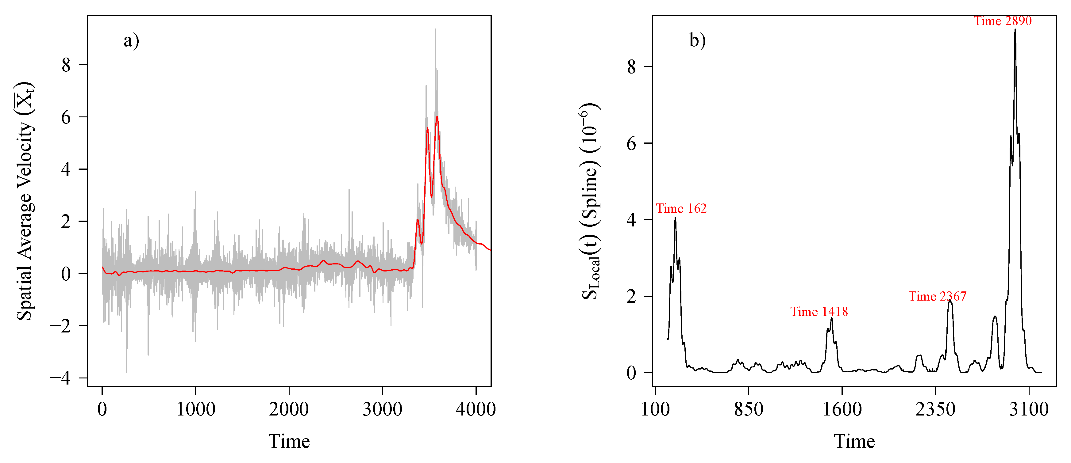
This section is an extension of stage two of our algorithm (Section 4.2.2). We describe further details of computation and discuss potential comparators.
  • In Definition 4, S ( t ) (3), we described that a value of S ( t ) is closer to 0 is indicative of second order stationarity (1) [12] of a time series. During a dynamic geological epoch feature time series, X s t , gradually evolve into higher degree non-stationary. To track the dynamics of change in the state of the system, as a function of time, we estimate S ( t ) over moving local time windows each of length 50, sequentially. Based on the trajectory of S ( t ) we partition the zone into two epochs. A period of relative stability for all times t < t 0 when S t < t 0 ( t ) is relatively close to zero and the unstable epoch t > t 0 with significantly higher values of S t > t 0 ( t ) . This leads to the estimated point of regime change, t 0 .
  • The problem of identifying t 0 in this algorithm is similar to that of estimation of change point(s) in time series. As such we could use any of a suite of methods for estimating t 0 . However, conventional approaches in change point estimation methods are commonly based on the variation in mean or trend and often require a priori assumptions on the (finite) number of change-points in the time series. See for example [29] and references therein. But it is quite well known that geological time series usually display non-stationarity in higher order statistical moments. Also, the rate of change (itself) is dynamic in time and space. Hence a better approach to studying variation in statistical properties would be to estimate deviation from second order stationarity as a function of time. Thus we suggest using S ( t ) as a characteristic feature of the zone for detecting the epoch change time, t 0 .
  • Here, we have implemented the non-stationarity metric on the smoothed velocity signal, V ( t n ) (Section 4.2.2). An alternative approach would be to use the non-stationarity metric S ( t ) to estimate the temporal variation of the dynamic Fourier transform of V ( t n ) (see for example [23] (Ch 4)), since the spectrum is a unique signature of a second order stationary time series.

Appendix B. Comparison of Non-Stationarity Based t0 against Subjective Choices

This section shows the table of observations corresponding to Figure 9 given in Section 5.4.2. The table compares the effect of non-stationarity based detection of t 0 = 2367 against 50 alternatives on subsequent estimation of times of emergent and imminent risk, t R and t I , respectively.
Table A1. Comparison of the risk ( U k ) and estimates of time of imminent risk t I for various choices of t 0 including times, 2342 and 2367 (red).
U k I k t I t R t 0
0.2490.093336327232342
0.2490.094342926682343
0.2490.093336627332344
0.2490.093335726682345
0.2490.093335826622346
0.2490.093335826662347
0.2490.095335726642348
0.2490.094335726612349
0.2490.093335726602350
0.2490.095335626642351
0.2480.092335526582352
0.2480.094335526642353
0.2480.096335526652354
0.2480.097335526652355
0.2470.099335326612356
0.2470.098335426602357
0.2460.095335424162358
0.2460.094335324102359
0.2450.094335326592360
0.2450.096335324132361
0.2420.098335326622362
0.2400.098335126652363
0.2400.099335126622364
0.2390.098335126642365
0.2390.094335126572366
0.2390.099335126602367
0.2370.099335126642368
0.2370.099335126612369
0.2360.095335126592370
0.2350.099335026632371
0.2350.096335126582372
0.2330.095335025882373
0.2330.094335025862374
0.2300.095293025902375
0.2300.097292626592376
0.2320.095292725862377
0.2280.095292928762378
0.2280.096292928762379
0.2300.102292828752380
0.2310.103336329702381
0.2290.106347729712382
0.2290.107347629732383
0.2350.107348129722384
0.2340.107347829722385
0.2350.107347829712386
0.2330.106347929732387
0.2330.105359029722388
0.2370.107358729712389
0.2370.108348131152390
0.2400.109348031162391
0.2400.107348231162392

Appendix C. Classification Details

This section provides additional computational details on classification of pixels, required in stage four of the Section 4.2.4 (see also Section 5.2).
We use the principle of likelihood maximization to classify each location (pixel) at all time points t 0 + 1 , t 0 + 2 , - post regime change- into one of the m baseline clusters ([32], Ch. 6). Akin to clustering, classification of the pixels are based on (cross-sectional) spatial variation of the features and do not account for temporal evolution. This allows classification of the locations without (temporal) bias.
For each location s let the classification set at times k = t 0 + 1 , t 0 + 2 , , , be denoted by P s k . P s k is a vector of multinomial probabilities. That is, at each time k > t 0 , P s k = ( p s 1 k , p s 2 k , , p s m k ) quantify the probability that location s be assigned to one of the m baseline clusters. Collectively, the probability matrix P k = { P 1 k , P 2 k , , P J k } describe the state of geological zone at time k. To estimate P s k we fit multinomial logistic regression models with the cluster labels as response variables and pixel velocity as covariate, using the principle of maximum likelihood. We expect that the state matrices, P k and P k at two different times { ( k , k ) : t 0 < k < k } during the epoch of high geological activity would be different. Further, this difference should gradually increase as the lag k k grows, till the event time t I , highlighting the increasing difference in the state of the system with the time of regime change, t 0 .

Appendix D. Distribution of Estimator for Uncertainty Parameter

In Section 4.2.5 and Section 5.3 we discussed that the first and second order moments of uncertainty (risk) metric U = p q share a parabolic relationship leading to a bilateral symmetric divergence of the beyond the time of emergent risk, t R . We now prove this using estimates of the mean and variance of p q . In Stage 5 of our algorithm, we use the following relationship between the maximum likelihood estimator of first and second order moments (mean and variance) of the classification uncertainty, M ( p ) = p q , to estimate the times of emergent and imminent risks, t R and t I , respectively.
Lemma A1.
If X 1 , X 2 , , X n are a sample of independent and identically distributed Bernoulli random variables with distribution,
f X i ( x i ) = p , i f   x i = 1 q = 1 p , i f , x i = 0
Then the mean of the maximum likelihood estimator for M ( p ) , M ^ ( p ) , and the corresponding variance, Var { M ^ ( p ) } , share a quadratic relationship given by,
M ^ ( p ) = p ^ q ^ = X ¯ ( 1 X ¯ ) ; X ¯ = i = 1 n X i E { M ^ ( p ) } = p q ( 1 1 / n ) Var { M ^ ( p ) } = Var { X ¯ ( 1 X ¯ ) } 1 n { p q ( 1 4 p q ) }
Proof. 
The first equality in equation M ^ ( p ) , follows from standard maximum likelihood theory for independent and identically distributed (iid) Bernoulli random variables. That is, the maximum likelihood estimator of p for n iid Bernoulli is X ¯ . Further, as p ( 1 p ) is a differentiable function of p for 0 < p < 1 , from the invariance theorem of maximum likelihood estimators we have of M ^ ( p ) is { X ¯ ( 1 X ¯ ) } . See for example [36].
Note   that , E ( X ¯ ) = p Var ( X ¯ ) = p q / n E ( X ¯ 2 ) = Var ( X ¯ ) + { E ( X ¯ ) } 2 = p q n + p 2 Hence , E { M ^ ( p ) } = E ( X ¯ ) E ( X ¯ 2 ) = p p q n p 2 = p q ( 1 1 / n )
Next we derive the variance. It is well known that if f ( X ) is a differentiable function of random variable X then
Var { f ( X ) } [ E { f ( X ) } ] 2 Var ( X )
The above relationship follows from Taylor series expansion and is commonly known as the Delta method, in statistics literature (see for example [37]). The method is often used to derive approximate variance of complex non-linear functions of a random variable. We have f ( X ¯ ) = X ¯ ( 1 X ¯ ) . Hence, f ( X ¯ ) = 1 2 X ¯ . Thus using Equation (A3) we have,
Var { X ¯ ( 1 X ¯ ) } [ E { f ( X ¯ ) } ] 2 Var ( X ¯ ) = 1 n { ( 1 2 p ) 2 ( p ( 1 p ) ) } = 1 n { p ( 1 p ) ( 1 p p ) 2 }
= 1 n { p q ( q p ) 2 }
= 1 n { p q ( q 2 + p 2 + 2 p q 4 p q ) } . But , ( q 2 + p 2 + 2 p q ) = ( p + q ) 2 = 1
Hence , Var { X ¯ ( 1 X ¯ ) } 1 n { p q ( 1 4 p q ) }
 □
It immediately follows that as a function of p q , Var { X ¯ ( 1 X ¯ ) } has its unique theoretical maximum and minimum at p q = 0.125 and p q = 0.25 , respectively (see Figure A1). In Section 3 we use the maxima and minima to obtain an estimate of t R (6) and t I (7), respectively. However our time varying risk estimates are based on the median ( U k ) and interquartile range ( I K ) of p q . In Lemma 1 we chose to use the mean and variance estimators of the uncertainty parameter p q for an algebraically simpler mathematical illustration of order O ( ) of the relationship between first and second statistical moments of U k . The order remains the same in both cases.
Figure A1. Relationship between the average uncertainty p q ( 1 4 p q ) / n and the corresponding variance p q (A7).
Remotesensing 11 02777 g0a1

References

  1. Sassa, K.; Matjaž, M.; Yin, Y. Advancing Culture of Living with Landslides—Volume 1 ISDR-ICL Sendai Partnerships 2015–2025; Springer: Cham, Switzerland, 2017. [Google Scholar]
  2. Peng, M.; Zhao, C.; Zhang, Q.; Lu, Z.; Li, Z. Research on Spatiotemporal Land Deformation (2012–2018) over Xi’an, China, with Multi-Sensor SAR Datasets. Remote Sens. 2019, 11, 664. [Google Scholar] [CrossRef]
  3. Pieraccini, M.; Miccinesi, L. Ground based Radar Interferometry: A Bibliographic Review. Remote Sens. 2019, 11, 1029. [Google Scholar] [CrossRef]
  4. Wasowski, J.; Bovenga, F. Investigating landslides and unstable slopes with satellite Multi Temporal Interferometry: Current issues and future perspectives. Eng. Geol. 2014, 174, 103–138. [Google Scholar] [CrossRef]
  5. Segoni, S.; Battistini, A.; Rossi, G.; Rosi, A.; Lagomarsino, D.; Catani, F.; Moretti, S.; Casagli, N. An operational landslide early warning system at regional scale based on space—Time-variable rainfall thresholds. Nat. Hazards Earth Syst. Sci. 2015, 15, 853–861. [Google Scholar] [CrossRef]
  6. Carlà, T.; Intrieri, E.; Di Traglia, F.; Nolesini, T.; Gigli, G.; Casagli, N. Guidelines on the use of inverse velocity method as a tool for setting alarm thresholds and forecasting landslides and structure collapses. Landslides 2017, 14, 517–534. [Google Scholar] [CrossRef]
  7. Intrieri, E.; Carlà, T.; Gigli, G. Forecasting the time of failure of landslides at slope-scale: A literature review. Earth-Sci. Rev. 2019, 193, 333–349. [Google Scholar] [CrossRef]
  8. Wikle, C.; Zammit-Mangion, A.; Cressie, N. Spatio-Temporal Statistics with R; Chapman & Hall/CRC The R Series; CRC Press: Boca Raton, FL, USA, 2019. [Google Scholar]
  9. Osmanoğlu, B.; Sunar, F.; Wdowinski, S.; Cabral-Cano, E. Time series analysis of InSAR data: Methods and trends. ISPRS J. Photogramm. Remote Sens. 2016, 115, 90–102. [Google Scholar] [CrossRef]
  10. Carlà, T.; Farina, P.; Intrieri, E.; Botsialas, K.; Casagli, N. On the monitoring and early-warning of brittle slope failures in hard rock masses: Examples from an open-pit mine. Eng. Geol. 2017, 228, 71–81. [Google Scholar] [CrossRef]
  11. Tordesillas, A.; Zhou, Z.; Batterham, R. A data-driven complex systems approach to early prediction of landslides. Mech. Res. Commun. 2018, 92, 137–141. [Google Scholar] [CrossRef]
  12. Das, S.; Nason, G.P. Measuring the degree of non-stationarity of a time series. Stat 2016, 5, 295–305. [Google Scholar] [CrossRef]
  13. Dick, G.J.; Eberhardt, E.; Cabrejo-Liévano, A.G.; Stead, D.; Rose, N.D. Development of an early-warning time-of-failure analysis methodology for open-pit mine slopes utilizing ground based slope stability radar monitoring data. Can. Geotech. J. 2015, 52, 515–529. [Google Scholar] [CrossRef]
  14. Gudehus, G.; Nübel, K. Evolution of shear bands in sand. Geotechnique 2004, 54, 187–201. [Google Scholar] [CrossRef]
  15. Pardoen, B.; Seyedi, D.; Collin, F. Shear banding modelling in cross-anisotropic rocks. Int. J. Solids Struct. 2015, 72, 63–87. [Google Scholar] [CrossRef]
  16. Amirrahmat, S.; Druckrey, A.M.; Alshibli, K.A.; Al-Raoush, R.I. Micro Shear Bands: Precursor for Strain Localization in Sheared Granular Materials. J. Geotech. Geoenviron. Eng. 2019, 145, 04018104. [Google Scholar] [CrossRef]
  17. Walker, D.; Tordesillas, A.; Pucilowski, S.; Lin, Q.; Rechenmacher, A.; Abedi, S. Analysis of grain-scale measurements of sand using kinematical complex networks. Int. J. Bifurc. Chaos 2012, 22, 1230042. [Google Scholar] [CrossRef]
  18. Tordesillas, A.; Walker, D.; Andò, E.; Viggiani, G. Revisiting localized deformation in sand with complex systems. Proc. R. Soc. A 2013, 469, 1–20. [Google Scholar] [CrossRef]
  19. Wessels, S.D.N. Monitoring and Management of a Large Open Pit Failure. Ph.D. Thesis, Faculty of Engineering and the Built Environment, University ofWitwatersrand, Johannesburg, South Africa, 2009. [Google Scholar]
  20. Harries, N.; Noon, D.; Rowley, K. Case studies of slope stability radar used in open cut mines. In Stability of Rock Slopes in Open Pit Mining and Civil Engineering Situations; SAIMM: Johannesburg, South Africa, 2006; pp. 335–342. [Google Scholar]
  21. Bavelas, A. Communication Patterns in Task-Oriented Groups. J. Acoust. Soc. Am. 1950, 22, 725–730. [Google Scholar] [CrossRef]
  22. Segalini, A.; Valletta, A.; Carri, A. Landslide time-of-failure forecast and alert threshold assessment: A generalized criterion. Eng. Geol. 2018, 245, 72–80. [Google Scholar] [CrossRef]
  23. Shumway, R.H.; Stoffer, D.S. Time Series Analysis and Its Applications: With R Examples, 4th ed.; Springer: New York, NY, USA, 2006. [Google Scholar]
  24. Lütkepohl, H. New Introduction to Multiple Time Series Analysis; Springer Science & Business Media: Berlin, Germany, 2005. [Google Scholar]
  25. Cressie, N.; Wikle, C. Statistics for Spatio-Temporal Data; John Wiley & Sons: New York, NY, USA, 2011. [Google Scholar]
  26. Schabenberger, O.; Gotway, C. Statistical Methods for Spatial Data Analysis; CRC Press: Boca Raton, FL, USA, 2005. [Google Scholar]
  27. Golub, G.H.; Heath, M.; Wahba, G. Generalized cross-validation as a method for choosing a good ridge parameter. Technometrics 1979, 21, 215–223. [Google Scholar] [CrossRef]
  28. Green, P.J.; Silverman, B.W. Nonparametric Regression and Generalized Linear Models: A Roughness Penalty Approach; CRC Press: Boca Raton, FL, USA, 1993. [Google Scholar]
  29. Killick, R.; Fearnhead, P.; Eckley, I.A. Optimal detection of changepoints with a linear computational cost. J. Am. Stat. Assoc. 2012, 107, 1590–1598. [Google Scholar] [CrossRef]
  30. Kaufman, L.; Rousseeuw, P.J. Finding Groups in Data: An Introduction to Cluster Analysis; John Wiley & Sons: Hoboken, NJ, USA, 2009; Volume 344. [Google Scholar]
  31. Maechler, M.; Rousseeuw, P.; Struyf, A.; Hubert, M.; Hornik, K. Cluster: Cluster Analysis Basics and Extensions; R Package Version 2.0.6—For New Features, See the ’Changelog’ File (in the Package Source). 2017. Available online: https://cran.r-project.org/web/packages/cluster/news.html (accessed on 21 September 2019).
  32. Anderson, T. An Introduction to Multivariate Statistical Analysis; Wiley: New York, NY, USA, 1958. [Google Scholar]
  33. Mann, M.E. On smoothing potentially non-stationary climate time series. Geophys. Res. Lett. 2004, 31. [Google Scholar] [CrossRef]
  34. Silverman, B.W. Some aspects of the spline smoothing approach to non-parametric regression curve fitting. J. Roy. Stat. Soc. B 1985, 47, 1–52. [Google Scholar] [CrossRef]
  35. Diggle, P.J.; Tawn, J.; Moyeed, R. Model based geostatistics. J. R. Stat. Soc. Ser. C Appl. Stat. 1998, 47, 299–350. [Google Scholar] [CrossRef]
  36. Zehna, P.W. Invariance of maximum likelihood estimators. Ann. Math. Stat. 1966, 37, 744. [Google Scholar] [CrossRef]
  37. Oehlert, G.W. A note on the delta method. Am. Stat. 1992, 46, 27–29. [Google Scholar]
Figure 1. (a) Monitored slope. (b) Spatial distribution of velocity at 13:10 15 June when the global average pixel velocity reaches its maximum during the entire monitoring campaign.
Remotesensing 11 02777 g001
Figure 2. (a) Velocity time series for the slip zone location with maximum velocity during event time. (b) Velocity time series for the stable zone location with minimum velocity at event time t E = 13:10 15 June.
Remotesensing 11 02777 g002
Figure 3. Flowchart of the proposed five-stage algorithm for characterization of the spatio-temporal evolution of pixel velocities over the studied domain D.
Remotesensing 11 02777 g003
Figure 4. (a) Time series of the global average spatial velocity scaled by the standard deviation (grey) with the superimposed smoothing spline estimate of the signal (red). (b) The corresponding non-stationarity trajectories.
Remotesensing 11 02777 g004
Figure 5. Cluster labels at different times: (a) t = 900 , (b) t = t 0 = 2367 , (c) t = t R = 2659 , (d) t = t I = 3350 , (e) t = t E = 3568 , and (f) t = 4000 . The red (blue) label has the highest (lowest) average velocity.
Remotesensing 11 02777 g005
Figure 6. (a) Risk of failure U k (4) (grey) for t 0 = 2367 . Dashed red lines are the lower and upper 95% confidence limits of U k obtained by fitting non-parametric smoothing splines to the trajectory of U k . (b) Variability of risk of failure I k .
Remotesensing 11 02777 g006
Figure 7. (a) Spatial mean (signal) of velocity time series across all 1803 locations. (b) Spatial variance (noise) of velocity time series across all 1803 locations. (c) Trajectory of signal to noise ratio. (d) Zoomed signal to noise ratio between times 3400 till 4000.
Remotesensing 11 02777 g007
Figure 8. (a) Risk of failure U k (4) (grey) for t 0 = 1418 . Dashed red lines are the lower and upper 95% confidence limits of U k obtained by fitting non-parametric smoothing splines to the trajectory of U k . (b) Variability of risk of failure I k .
Remotesensing 11 02777 g008
Figure 9. Estimated values of t I (7) and t R (6) for 51 different choices of t 0 . Non-stationarity based on t 0 = 2367 (3) is compared with 25 prior and subsequent time points, Panel (a) shows estimates of t I against t 0 , (b) plots t R against t 0 . The intersecting lines show the estimates obtained using the algorithm.
Remotesensing 11 02777 g009
Table 1. Explained intra- and inter-cluster variations for different numbers of cluster partitions, 2 , 3 , 4 , 5 , at non-stationary times, t = 2367 and t = 1418 . Time point t = 2367 has a higher explained inter-cluster variation for a smaller cluster solution. It is selected as t 0 .
TimeNo. of ClustersWithin Cluster VariationExplained Inter-Cluster Variation (%)
236720.1470.080 74%
30.0400.0550.028 86%
40.0160.0210.0190.028 90%
50.0180.0070.0200.0050.01193%
141820.0190.015 53%
30.0050.0170.003 67%
40.0040.0040.0140.002 69%
50.0030.0020.0040.0030.00281%

