1. Introduction
An important application of remote sensing is the observation of ocean phenomena on scales from local to global, such as tsunami propagation generated by major earthquakes. The catastrophic Asian tsunamis of the last 15 years caught the world’s attention, with the 2004 earthquake at Banda Aceh, Indonesia claiming a quarter of a million lives. The detection of the earthquake itself of course gave a general warning of the danger, but in this case, no local warning of the magnitude of the impending disaster was available. There are now many methods used in tsunami detection: the continuous monitoring of seismic events with modeling, changes in the tide level, detection by open-ocean buoys and coastal tide gauges and by using pressure recorders located on the ocean floor [
1,
2,
3,
4,
5,
6,
7,
8,
9,
10,
11]. In this paper, we describe the quantitative modeling of local tsunami behavior and its detection using a shore-based HF radar system. This approach has the advantage of giving local warning without requiring hardware in the ocean, which contributes to its reliability. The tsunami need not be generated by a major earthquake, as was the case in the 2018 event near Krakatoa [
12] and the 2013 meteotsunami off the east coast of the US [
13].
HF radars were first used to provide ocean observations in the 1960s. Located on the coast and transmitting vertically polarized radiation, they exploit the high conductivity of sea water to propagate their signals well beyond the visible or microwave-radar horizon. They have found widespread use for mapping surface currents and monitoring sea state and are under development for tsunami detection. Barrick [
14] suggested in 1979 that HF radar networks deployed for surface-current mapping could detect tsunamis by means of their orbital wave velocity as they approach the coast. The primary interest in tsunami warning has been to detect and forecast its height, rather than its velocity. Little was done to develop this capability until the 2004 earthquake at Banda Aceh, when work began to quantify the radar tsunami response. It was not until the 2011 Japan tsunami that sufficient radars were in place to capture real-time tsunami data, which was used to develop algorithms for detection and warning, based on pattern-recognition in the velocity time series. The use of HF radar systems deployed on coasts to give tsunami warning is described in [
15]. The Japan tsunami signal was also observed by a number of HF radars around the Pacific rim with clear results from many sites in Japan and USA [
15]. Since that time, additional weak tsunamis have also been observed [
15].
With the deployment of hundreds of HF radars operating worldwide, it has become clear that some sites are less suitable than others for tsunami monitoring by radar, as the tsunami signature can be masked by large, variable background currents. Tsunami detection is favored by shallow water extending far offshore and by slowly varying background current fields. In this paper, we provide details of the use of partial differential equations (PDEs) to simulate tsunami velocities/heights. We also describe a method for the evaluation of a coastal site for tsunami warning based on the superposition of simulated velocities on measured current velocities, which allows us to estimate the minimum height of a tsunami that can be observed by the radar at that site. This method is illustrated by application to a short data set from a radar system installed at Brant Beach, New Jersey (BRNT).
The first indication of a tsunami might be the seismic detection of an earthquake. As not all subsea earthquakes produce tsunamis, extensive modeling is required to forecast the detailed generation or intensity of a resulting tsunami. At present, the only operational sensor that detects a tsunami and measures its intensity is a bottom pressure sensor connected to a buoy overhead. Developed by NOAA (the National Oceanic and Atmospheric Administration), networks of these sensors called DART™ (for Deep-ocean Assessment and Reporting of Tsunami) were deployed after the 2004 event. They observe the height of the tsunami wave as it passes above them. The tsunami height measured by these buoys is then entered into numerical tsunami models [
3,
16] to give rough forecasts of the tsunami arrival time and intensity at coastal points around the world. As this network is located in the deep ocean, not all tsunamis are observable by DART and these may not be entered into the model before coastal impact. Furthermore, the model’s forecast of intensity at the coast is often coarse, so that more accurate estimates of intensity at specific locations are needed; such local variations not captured by the models are referred to as “near-field”. HF radars make their areal observations over this local near field and so provide an ideal solution for this need.
Because of its long wavelength, the tsunami’s orbital velocity appears as part of the surface current as the wave approaches the coast. Tsunami periods lie typically between 10 and 40 min. This requires real-time sampling and processing of received HF radar echo every few minutes. A tsunami has its origin as a massive displacement of water: usually over a large area but with small vertical dimensions. These include subsea earthquakes where plates force each other upward/downward, respectively, subsea landslides along steep submerged mountainous slopes or fast-moving atmospheric anomalies (e.g., low-pressure centers) that create “meteotsunamis”. As the displaced water mass leaves its source region under the influence of gravity, it becomes a freely propagating shallow-water wave. Although the origins of meteotsunamis vis-a-vis seismically generated tsunamis differ, the propagation and evolution of these shallow-water waves are the same, as are the applicable detection and warning methods. Because of the diversity in local bathymetry, there is considerable variation in the warning-time available, primarily depending on the width of the adjoining continental shelf. Warning-times vary from minutes on the US Pacific coast to hours for some areas of the Atlantic coast and South East Asia.
This paper is organized as follows:
Section 2 provides a general background on the use of coastal HF radars for current velocity mapping; radar tsunami detection is based on the analysis of current velocities.
Section 3 describes modeling of tsunami heights and velocities in the near-field region of coastal HF radars.
Section 4 outlines the averaging of radial velocities in rectangular area-bands and shows examples of simulated area-band velocities and heights for BRNT.
Section 5 describes a method to use the simulated current velocities as they appear in the bands to predict the minimum tsunami height; this method is illustrated by application at BRNT for a 24 h period.
2. Radar Current Velocity Mapping
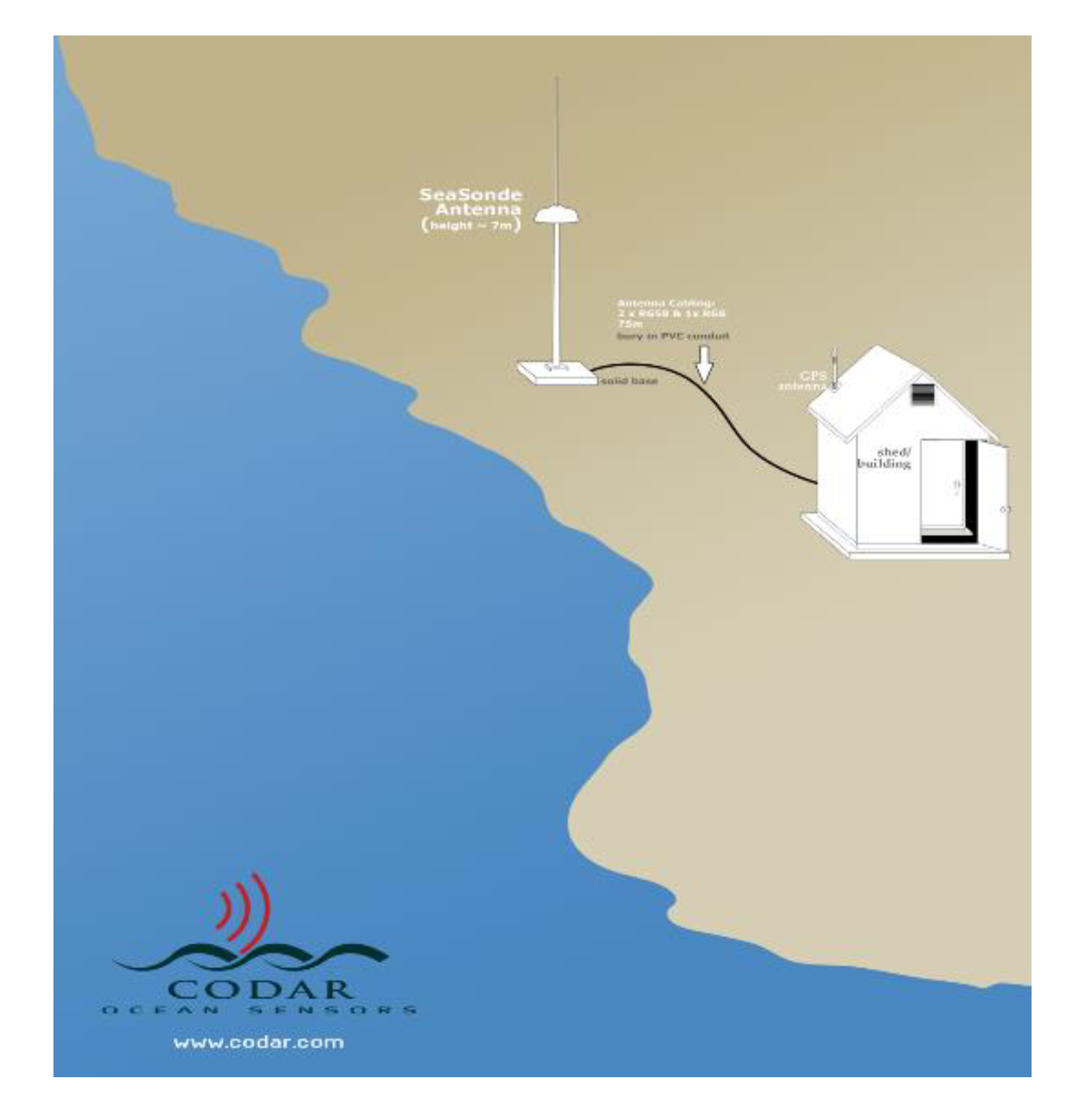
HF radars differ from their far more common microwave cousins in their wavelength (or frequency). With wavelengths between 100 and 10 m (frequencies from 3–30 MHz), the first very large radars built in the 1930s were HF, before modern-day miniaturization was possible. Today, over two billion microwave radars exist, compared to several hundred HF radars worldwide. A sketch of a coastal CODAR SeaSonde radar arrangement is shown in
Figure 1.
2.1. Antenna Size
A distinguishing feature between radars in these two bands is their antenna size and how they determine target bearing. The well-known way to detect a signal’s angle is to radiate/receive through a spatial aperture many wavelengths in extent. This causes a narrow beam to be formed and scanned in direction. Beam width in radians is roughly the wavelength divided by the spatial width across the antenna aperture. While this leads to microwave parabolic dish antennas that are a couple meters across, the counterpart at HF is an array antenna as much as a kilometer in length, called a phased array. The first HF radars based on antenna-array principles were produced in the 1960s for military target surveillance. Rather than using mechanical scanning, the phased array adjusts the phases to the individual antenna elements to digitally form and scan its beam, with typical beamwidths greater than 10°. Such huge arrays near public shoreline were considered to be undesirable, which motivated NOAA to invent smaller broad-beam radar systems [
17]. The use of a compact receiving antenna precludes beam forming to determine angle, as the beam width would be many tens of degrees, which would destroy the required bearing resolution. Therefore, compact antenna elements were adopted that used direction-finding rather than beam forming. One arrangement for the SeaSonde
®, a commercially available HF radar, involves two crossed loops mounted inside a dome, see
Figure 2, and a coaxially aligned vertical monopole or dipole element. Direction finding is based on the orthogonal patterns of the loops. Even when patterns are distorted, their measurement after installation allows accurate bearing estimates. See [
18] for more detail.
2.2. Signal Propagation
A second significant difference between microwave and HF is the propagation mode, or path. Electromagnetic waves with frequencies above ~500 MHz, both microwave and optical, travel along straight lines and are blocked by obstacles. HF waves bend away from straight lines, for example following the curvature of the earth to propagate over the sea beyond the horizon. These are HF surface-wave radars (HFSWR); the electric field polarization must be vertical and the surface conductivity high. Moving over the sea, which has high surface conductivity due to its salinity, such surface waves attain distances of hundreds of kilometers beyond the visible horizon; the lower the frequency the greater the range.
Another mode of HF propagation is ‘skywave’, for which signals with frequencies less than ~50 MHz are refracted by the charged ionosphere, with altitude from 80 to 400 km. Acting like a mirror, this redirects the signal back to the earth, allowing propagation distances as large as 4000 km. Such signals are useful for radio communication and some very large military surveillance radars, called OTH (over-the-horizon) radars. Ionospheric motions preclude their use for precise wave and current monitoring. Skywave signals from other sources can negatively impact HFSWR operations because they constitute radio interference and noise that limit performance.
2.3. Antenna Location vs. Propagation
HF signals that propagate along paths near the ground are very sensitive to the earth constants. Vertical polarization is required. Attenuation over the earth is much greater than that over conducting sea water and increases with frequency: Tens of decibels are lost in propagating above normal earth. As a result, HFSWR antennas for coastal observations must be located very close to the water. Locations more than 100 m from the coast produce significant signal loss. Raising the HF antenna does not improve this situation, as it does for microwave radars. Hence, site location selection is a critical factor in planning permanent site installations. The US surface current mapping network [
19], which has been in place for 15 years, was intended to display slowly moving near-shore current fields on public websites. It consists of many systems similar to the device in
Figure 2.
3. Modeling Tsunami Flow
Tsunamis have four main origins: (i) seismic, meaning subsea earthquakes; (ii) meteotsunamis produced by atmospheric fronts passing across the coastline; (iii) sudden subsea landslides at mountains below the surface; and (iv) volcanic eruptions causing water displacement.
At this point, hundreds of coastal HF radars worldwide are in operation, which can capture the signals during tsunamis, leading to the development of detection/warning algorithms [
15]. We outline limitations in some existing methodology; it is important to understand and mitigate these before integration into national tsunami warning center forecasts. To clarify these limitations, in this section, we describe modeling of tsunami flows in the near-field region close to the coast.
3.1. Tsunami Features in the Near-Field
A tsunami is typically a shallow-water wave, meaning that its wavelength is much greater than water depth. A radar measured the horizontal component of the tsunami orbital velocity. Bathymetry and the coastal geometry play crucial roles in tsunami detection by a coastal network. They impact warning time and how far away a tsunami of given intensity is visible in this ‘near field’. Tsunamis are rare events and it is impractical to wait for observations only at specific coastal points in order to estimate performance. Because of large variations in depths and coastal geometries, one cannot give a single universal specification for an HF radar tsunami sensor system. The lack of required operational information limits the capability to predict the estimated performance of radar tsunami-detection for important populated areas. For a given tsunami intensity, the range possible for its detection depends on the offshore bathymetry and the frequency band of the radar.
As mentioned above, tsunamis have temporal patterns with time scales and periods of the order of 10–40 min, requiring real-time sampling and processing every 2–4 min. This information must be output more rapidly than is done for the general current velocity pattern work performed by many of the present coastal networks. Furthermore, tsunamis must be detected against a background of other slower-moving features with the maximum possible sensitivity. We begin by examining the nature of any tsunami in this coastal near field extending out tens of kilometers and illustrate this by providing examples.
3.2. Simple Models
We now consider two simple models for wave refraction: the first is provided by ray-optics, which allows the wave-propagation direction cosine to change inversely with refractive index (proportional to the square root of the depth); the second (Green’s Law) has the dispersion relation changing so that wavelength is proportional to this refractive index. Both of these fail when depth changes rapidly with distance along the ray path with respect to the tsunami wave’s horizontal scales.
3.2.1. Modeling for Water with Near-Constant Depth
We first consider a tsunami passing over a shelf of near-constant depth D. As a shallow-water wave, this means that the tsunami wavelength is much greater than depth; this holds for a tsunami even over the deepest parts of the ocean).
In the linear approximation, the phase speed of
(
d) in water of arbitrary depth d is given by
where
g is the acceleration of gravity (~9.8 m/s
2).
The time
T for a tsunami to cover a distance L terminating at the radar site, is given in terms of the phase speed by
The orbital or water particle speed
for wave amplitude
a and water-depth
d is given by
The two speeds (1) and (3) in water of depth D are very different from each other. The wave-crest phase speed does not, its amplitude. Consider the following example: Take a shallow-water depth of D = 40m, and a tsunami of crest amplitude A = 1.0 m at that depth. Its phase speed is ~20 m/s or 72 km/h. This is the speed that the tsunami crest propagates at this depth. As seen from the equation in the linear approximation, this does not depend on the tsunami’s amplitude, but only on the near-constant water depth.
In contrast, its orbital speed, , is ~0.5 m/s. This is the speed of a particle drifting on the surface. It is also the speed of the short Bragg wavetrain seen by an HFSWR as it propagates on top of the tsunami crest. This is the tsunami target speed that the radar must detect above noise and all other background flows, e.g., tidal flows. This velocity is in the range of detectability by HFSWR when the echo falls above background noise.
In the above example, a tsunami of 1 m height in a water depth of 40 m is considered to be quite strong. We will now show how this changes as bathymetry on the shelf becomes shallower.
An important feature of any tsunami is that its orbital/particle speed is constant with depth. This result can be obtained from an analytical derivation starting with the three-dimensional velocity potential,
. The depth
z is taken to be positive downward;
z =
D defines a constant-depth bottom. For illustration, here, we consider one-dimensional flow in the
x direction. Flow velocity in a given direction is defined as the partial derivative of velocity potential with respect to
x and
t. This leads to the following equation for particle flow in the shallow-water column in direction
x as
where the frequency
is related to the tsunami period
as follows:
In the derivation of (4) the following assumptions are made:
The hyperbolic factor in (4) contains the dependence of tsunami flow on depth. For a typical 40-min period, at the mean surface, z = 0, the above hyperbolic factor has the value 1.000013986, while at the bottom, z = 40 m, the hyperbolic function is exactly equal to 1. It follows that the orbital/particle-current variation with depth for this case is close enough to unity to be negligible, i.e., tsunami flow can indeed be considered independent of depth.
The cosine factor in (4) represents the movement of the tsunami hump as a traveling wave. For the previous example, the speed is 72 km/h as dictated by the water-depth of 40 m.
3.2.2. Modeling for Slowly Changing Water-Depth
We next consider a water depth that changes slowly with horizontal distance. Kinsman [
20] shows that a very shallow-water wave, starting at depth
D, the amplitude
a will vary with depth
d as follows:
where
A is the initial crest amplitude.
Following our previous example, starting with amplitude 1 m at depth 40 m, we consider moving closer to the coast to the point where depth decreases to 2 m. Now, the tsunami amplitude given by (6) becomes ~2.1 m. It has essentially doubled over the depth change from 40 m to 2 m.
From (3) and (6) its orbital speed follows the law:
For our example, the orbital velocity given by (7) becomes ~1.50 m/s. Thus, while the tsunami height has essentially doubled as we move in from 40 m to 2 m depth, the orbital velocity, which is measured by the radar, has tripled. This example illustrates that as water depth decreases, the radar observable, i.e., the orbital velocity, is a considerably more sensitive tsunami indicator than its height. HFSWR can easily detect a radial current velocity of 1.5 m/s.
However, this “behavior” depends on depth changing very slowly over the spatial scales of the tsunami, which is normally not the case. This is often overlooked in analyses of HFSWR tsunami detectability and modeling. When it is true, the tsunami wave is said to obey the Green’s law and ray optics approximations. See [
15]
Section 2 and
Section 3 for further discussion and examples.
3.3. Modeling Near-Field Tsunami When Depth Change is Sharp
We now describe a partial differential equation (PDE) methodology that overcomes the two approximations described in
Section 3.2 that are often used incorrectly to model tsunami propagation across a bottom with varying depth. The more common situation is that the near-field, coastal HFR tsunami detection zone contains the steep continental slope at the shelf edge. This abrupt change in depth does not allow good modeling accuracy based on the approximations outlined in
Section 3.2 (i.e., Green’s law and ray optics). We have developed a linear numerical model based on the simple equations of motion, which is suitable for solution in this situation using desktop computers. The basis of the model is outlined below. This PDE methodology is linear until very near shore where breaking begins to occur.
3.3.1. Hydrodynamic Equations
In this section, we describe the basic hydrodynamic equations used in the development of the model.
Conservation of mass and incompressibility of water:
As an HF radar is a fixed sensor, it measures Eulerian current velocities. We now consider a water column of small lateral dimensions compared to a tsunami wavelength, extending over the full depth of the water. Since water is essentially incompressible, conservation of mass gives rise to the equation:
where
mean water depth, depends on horizontal distances but is independent of time
height of tsunami wave, which is dependent on time;
horizontal water particle (orbital) velocity, which depends for a tsunami on time and horizontal position, but not on vertical position, see (4) above. Equation (8) can be interpreted as follows: the left side denotes the horizontal rate of change of water flow with position of the water column. This must be balanced by a rate of change in the height of the water column, as given on the right, in order to conserve the water volume in the column, as the water density is constant.
Equation (8) assumes that the timescale for changes in the tsunami flows is significantly shorter than that for changes in the background currents, allowing the latter to be neglected for the type of modeling described here. The tsunami hydrodynamic equations we use in the near field are linear, as are the equations for tides and geostrophic flows to lowest order. The scales for tsunami (time and space) are smaller than the other background effects they are competing with: (a) for tsunami, tens of minutes and tens of kilometers (up to ~100 km in near field); (b) for tides, time scales ~12–24 h and hundreds of kms in space; (c) for geostrophic flows (e.g., Gulf Stream eddies), days in time and hundreds of kms in space. Being linear means the coupling of these processes can be neglected and their equations can be added linearly and independently. The HF radar’s signals and their processing can thus sort out and separate tsunami effects from other background currents because of their different scales.
Equation of motion:
The equation of motion for the free surface is easily obtained from Newton’s second law. For moving water bounded on top by a free surface and by a rigid bottom, the linearized momentum equation can be expressed as
Acceleration is the rate of change of horizontal velocity, expressed on the right side of (9). Gravity acting on the slope of the sea surface on the left exerts the force needed to accelerate the water horizontally in the direction of the maximum slope of the wave. Different derivations than simple Newton’s law are possible but unnecessary in this case. For example, in hydrodynamics this is also the lowest order version of the Navier-Stokes equations [
21].
3.3.2. Partial Differential Equation for Tsunami Wave Height
Equations (8) and (9) represent two equations in two unknowns: the tsunami wave height and the orbital velocity. These can be combined to eliminate either of the unknowns, resulting in a second-order partial differential equation, either for the tsunami shallow-water wave height or the wave orbital velocity. If we first solve for the height, the velocity can then be obtained from (8) or (9).
The problem is further linearized by dropping the height
from the square brackets on the left side of (8). This is permissible because tsunami height is typically very small in terms of the mean water depth
within the radar coverage area (e.g., many meters deep compared to a fraction of a meter for tsunami height). We then obtain the following PDE, which is linear in terms of the height.
The solution of (10) forms the basis of our near-field tsunami modeling.
3.3.3. PDE Solution Using MATLAB™
For an uneven bottom, numerically methods are generally required to solve Equation (10), which is a second-order hyperbolic PDE. Hyperbolic PDEs, owing to the negative sign separating the two terms, lead to propagating waves as solutions, e.g., a tsunami. A MATLAB “toolbox” specifically solves PDEs [
22]. We discuss below the germane assumptions and illustrate with an example leading to a movie of simulated tsunami results for the U.S. East coast, where a number of SeaSonde HFSWRs have been operating in real time for over a decade for current velocity mapping.
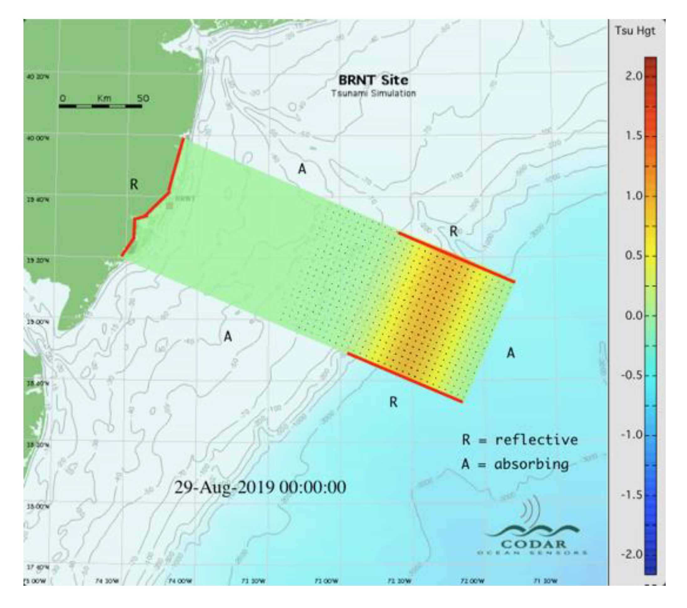
PDE Solution Domain
A bounding box (or computational domain) is defined around the coastal region of interest for modeling.
Figure 3 illustrates this in map form, showing subsea bathymetry offshore from the radar site BRNT. The rectangular box extends to the SSE about 240 km, where the depth exceeds 1000 m. The region with densely bunched isobaths is at the edge of the shelf, where the slope is known as the continental slope. There approximations discussed earlier in
Section 3.2 are expected to fail, while our linear PDE method overcomes this limitation. This box comfortably contains the HFSWR radar coverage area for the 13-MHz systems installed along the New Jersey coast, where the maximum range is typically 85 km offshore. The bounding box has fixed flat walls except at the coast and a fixed bottom shape that is included exactly based on available bathymetry databases, while the free upper surface is one of the variables (tsunami wave height) that we are solving for. The first step in code execution fills the box with a variable-size triangular grid, with the solution to be determined at the center of each triangle. This is a well-known step in numerical solutions of PDEs, called Finite Element Modeling [
22].
Boundary Conditions
The solution of the PDE requires boundary conditions to be defined. The bounding box is an artifact that allows us to approximate reasonable boundary conditions for the algorithm, based on the tsunami space and time scales. In this case, the boundary is defined by the sides of the box. Our extension of the MATLAB code allows for two boundary conditions: (i) Reflecting (denoted by the red edge-regions of the box), mathematically referred to as a Neumann (hard) boundary. Here, these extend along the coastline (to the left) and the sides of the box farther out, the latter to prevent the initial leaking of the tsunami beyond those boundaries. (ii) Absorbing, where the tsunami wave solution can penetrate with no reflection back. Mathematically this is referred to as a radiation boundary condition. The tsunami will propagate toward the coast, so we do not want any reflections from the back of the box nor the regions on the box sides closer to the coast. Here, the energy is allowed to leak out based on the flows controlled by the bottom contours. Selecting the location of these boundaries required some experimentation.
Initial Conditions
Because (10) represents a wave propagating forward in time, initial conditions are required. As the PDE is second-order, two initial conditions are required. The initial condition is depicted in
Figure 3 as the orange ridge of vector arrows with yellow edges to the right in the box. If the tsunami source is far from the coast, it can be defined initially as a plane wave, or ridge, starting in deep water at ‘zero time’. The two initial conditions define the initial tsunami height and its temporal derivative: i.e., the horizontal velocity. For the situation shown in
Figure 3, the height of the ridge center at the start is set to 1.0 m (i.e., it is normalized). Its time derivative represents a wave horizontally propagating at the phase speed corresponding to the depth below the ridge. From these initial conditions, the code calculates height and velocity at each point and time step onward.
In addition to a ridge or plane wave, we have the option of a ‘point-source’ initial condition. This could represent a subsea earthquake and would cause the water above it to rise as a hill. As gravity exerts its force, initially the surface perturbation propagates away in a circular fashion. These circles become distorted contours as the irregular bathymetry modifies the refractive index and wave speed for propagation in different directions.
Denormalization
Our extensions of the basic MATLAB “hyperbolic(X,Y,…,Z).m” function that solves the PDE carry along not only the height, from (10), but also the orbital velocity, obtained from numerically applying (3) to the height field. We start with normalized elevation set to 1.0 m at the initial-condition height maximum. The correlations between height and velocity are carried along within the coding. Therefore, both the derived velocity and height fields are correct over space and time, apart from a multiplicative constant. In the next denormalizing step, that constant is specified by the user, relating the normalized height at a convenient point in the field (e.g., close to the shore where a “hazard” value might be specified) to be the desired height at that point. Then all points in space and time are multiplied by this constant to denormalize, giving the actual velocity (e.g., m/s) and height (e.g., in m).
Depiction of Outputs/Movies
Outputs from the code are files of tsunami height and orbital and/or total velocity, mapped as a function of time for each step forward.
4. Band-Representation of Simulated Tsunami Velocities and Heights
Simulated tsunami velocities are based on PDE modal solutions of equations of motion. The initial wave height is set to 1.0 m. To set the initial waveheight to have some other value, e.g., 10 cm, then all modal vectors and wave heights are multiplied by a factor F = 0.1 in each set of data files.
Radial velocities are averaged in rectangular area-bands 2 km wide approximately parallel to the depth contours. BRNT area-bands used in this analysis are shown in
Figure 5.
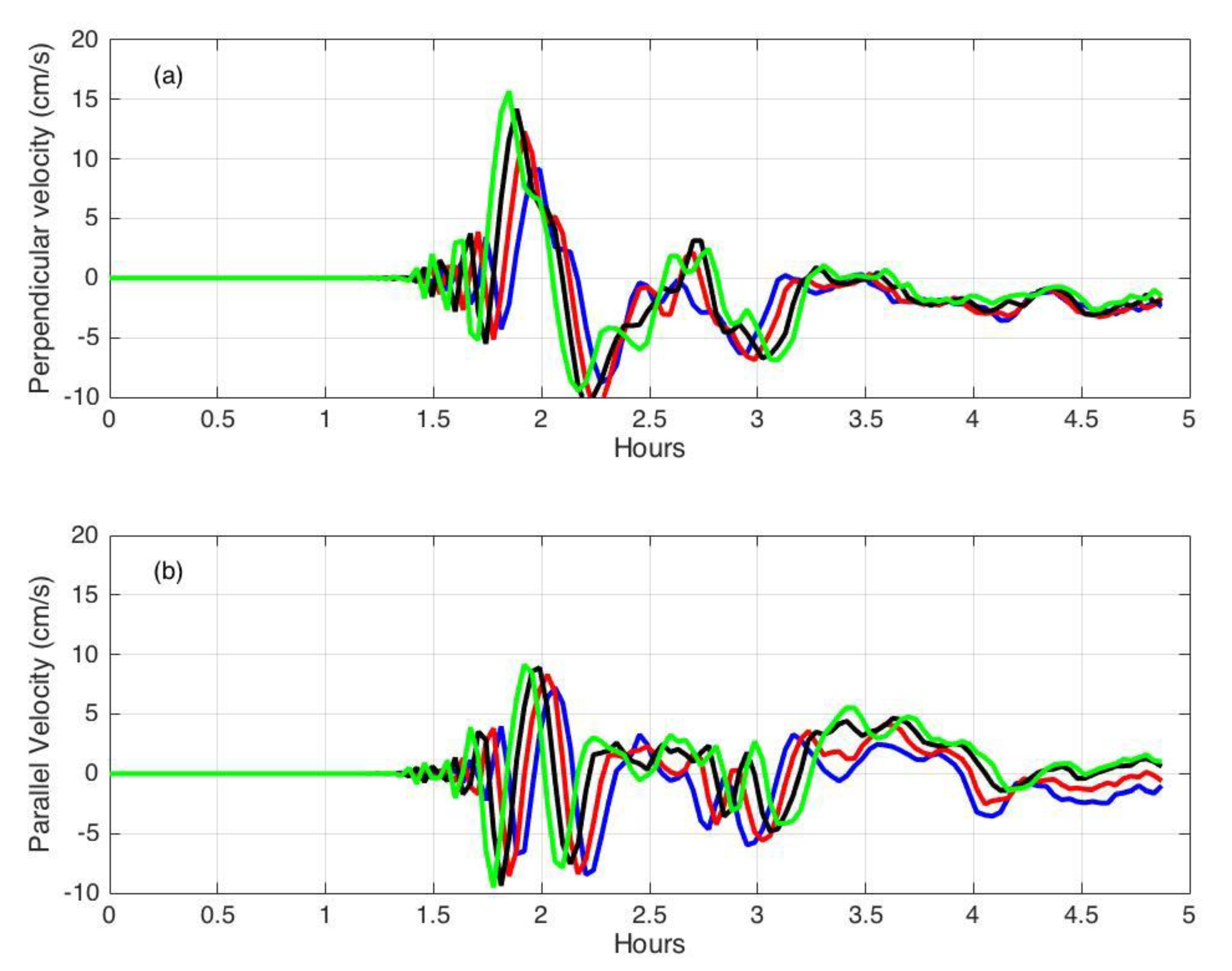
Simulated BRNT radial velocities are resolved into components perpendicular and parallel to the area-bands. These components are averaged over the band and are termed ‘band velocities’. Time series of the band velocities/heights are then formed, which display the characteristic oscillations produced by the tsunami.
Figure 6 shows time series of simulated band velocities (
Vsim) obtained over a 5-h period.
Figure 7 shows a magnified view of the area-band velocities around the time that the tsunami approaches the coast.
The approach of the tsunami toward shore is indicated by the increase in the perpendicular velocity component and the correlation in time between velocities in different area bands. Due to the decreasing water depth as the coast is approached, the tsunami arrival time differs by about 3 min between these adjacent area bands.
For comparison with the simulated results,
Figure 8 shows observed band velocities perpendicular to the band boundary for a meteotsunami that approached BRNT on 13 June 13 2013 [
13].
For this case, negative velocity means water is moving offshore; the observed velocities indicate the tsunami arrival by a marked drop in the perpendicular velocity component as different parts of the tsunami wave are being observed and shows correlation in time between different area bands. No tsunami signature was observed in the parallel component.
Simulated BRNT tsunami heights were averaged over each band; results are shown in
Figure 9.
5. Evaluation of Radar Sites for Tsunami Detection Using Simulated Tsunami Velocities
As some sites are less suitable than others for tsunami monitoring using coastal radar systems, we are developing a site-dependent method that uses simulated tsunami velocities to estimate the size of a tsunami required to trigger a detection as a function of distance from the shore. This leads to an estimate of the warning time available, as a measure of performance. This section describes the present status of this method and gives an example of its application at BRNT over a period of one day.
Two effects distinguish tsunami velocities from the background: (a) velocities in neighboring bands are strongly correlated after the arrival of the tsunami, (b) the velocity oscillations are clearly visible above the background. These effects appear to be characteristic of tsunami band velocities, as they occur in all the tsunami radar data that we have analyzed, see [
15]. They form the basis of a simple pattern detection procedure. At a given time, a factor (which we call the
q-factor) is defined which signals the tsunami detection when it exceeds a preset threshold. See [
15],
Section 3.3 for a description of the detection method.
5.1. Site-Evaluation Method
To evaluate a site for tsunami detection, initially, the radar system is run for an extended period of time to generate a suite of measured radar spectra. Tsunami detection software is then used to calculate q-factors. From this, we form an estimate of the q-factor values observed in the absence of tsunamis. Next the PDE-simulated radial velocities obtained over a 5-h time period are converted to band velocities (VSim).
Then the following steps are carried out for sliding 5-h time periods to estimate the size of an approaching tsunami required for detection at the test site.
Step 1: The test site is assumed to be operating in its normal current-mapping mode acquiring radial velocities, which are converted to band velocities VSite over the 5-h time period.
Step 2: The reference set Vsim are multiplied by a factor F and added to VSite to produce combined velocities Vcomb, which are analyzed to produce q-factors, using the tsunami detection algorithm. This is repeated for a range of increasing values of the factor F, representing increasing tsunami intensity. The minimum value of F (Fdetect) is sought that will lead to detection of the q-factor peak. Tsunami heights corresponding to the q-factor values Fdetect are then calculated. These define the minimum height of a tsunami that can be detected at that radar site.
Step 3: The warning time provided by each band with a detection is calculated from (2).
Step 4: Steps 1–3 are repeated using a sliding 5-h time window that can run in the background of an operating HF radar system. This provides results over an extended time period which can be used to estimate the q-factor threshold for defining a detection.
Tsunami periods typically lie between 10 and 40 min. This requires real-time sampling and processing of received HF radar echo every 2 min. The tsunami detection method used at present analyzes band velocities over four adjacent time intervals and four adjacent bands. It can therefore be applied independently of the tsunami period.
5.2. Application of the Site-Evaluation Method at BRNT
We now give an example of application of the evaluation method at BRNT. Initially, tsunami detection software was run with measured radar spectra for a 24-h time period from 29 September 2019, 18:00 to 30 September 2019, 18:00. The resulting q-factors obtained were less than 200. The threshold q-factor value defining a tsunami detection was then set to 400.
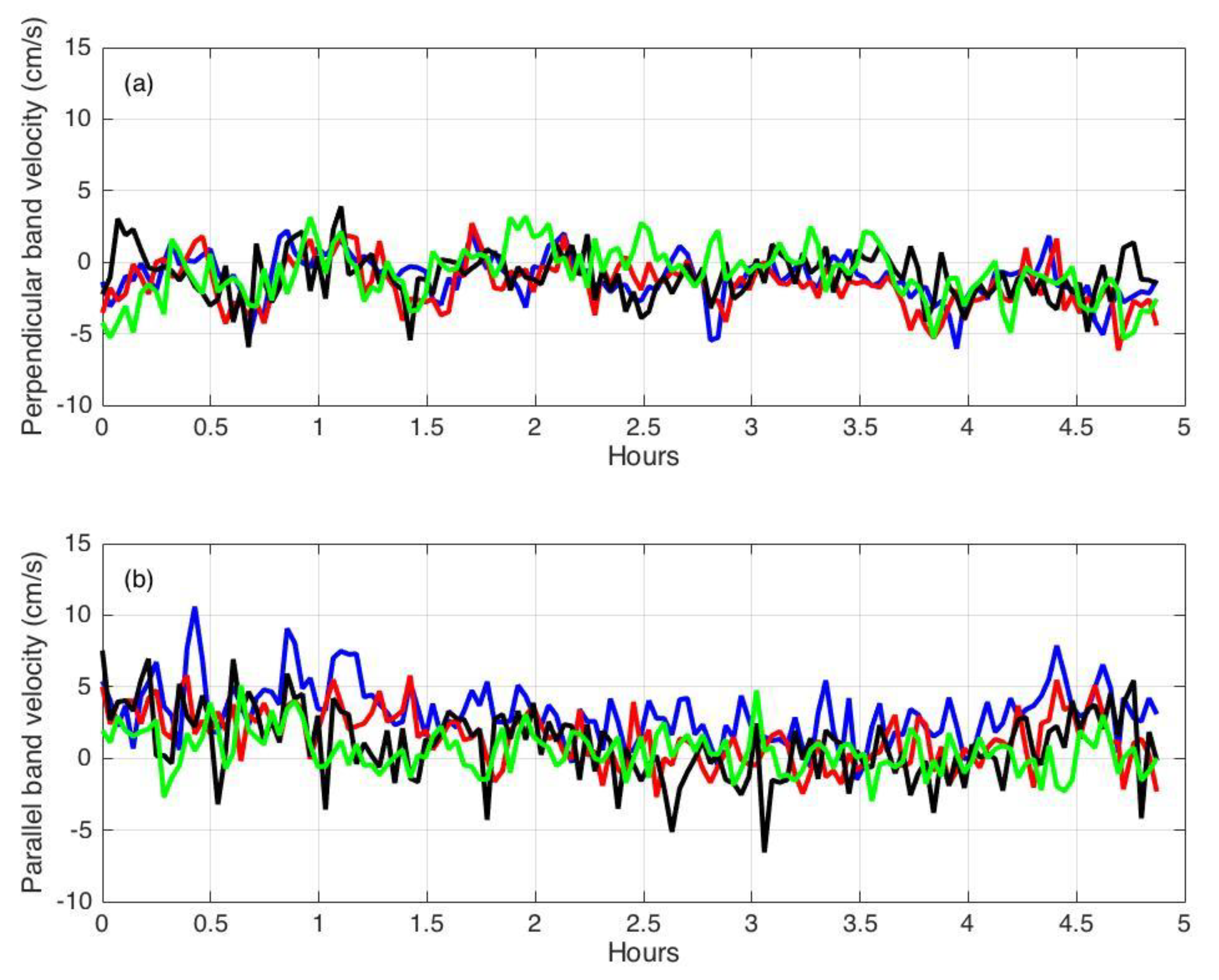
Step 1 (BRNT): Measured band velocities (VSite)
Radar-echo cross spectra measured over 5-h periods were analyzed to give area-band velocities. An example of measured area-band velocities, perpendicular and parallel to the band boundary over a 5-h period, is shown in
Figure 10.
Step 2 (BRNT): Combined velocities
Vcomb were created by multiplying the simulated band-velocities by a factor F and adding them to the site velocities, which are then analyzed to give band velocities and
q-factors. Each
q-factor value obtained comes from analysis of four adjacent spectral sidebands. The factor F was increased to a value
Fdetect which resulted in an acceptable detection of the
q-factor peak, with a
q-factor value greater than the limit of 400 set for BRNT.
Figure 11 shows the resulting band velocities
Vcomb and
q-factors for the same 5-h time window shown in
Figure 10.
The following maximum q-factors were obtained: Band 2: 6300, Band 3: 3300, Band 4: 1400, Band 5: 400. As these values meet or exceed the set q-factor threshold limit, there was a detection provided by the velocities in Bands 2–5. The maximum q-factor values increase as the water depth decreases as the shore is approached.
Step 3 (BRNT). The time-to-shore of the tsunami from the inner side of the bands was calculated from (2) with results as follows. This agrees with the time progression for each frame calculated from the PDE-simulation code:
Band 2: 6.8 min
Band 3: 11.0 min
Band 4: 14.4 min
Band 5: 17.3 min
This warning time could be used to alert people to move immediately to a safe place as high and as far inland as possible. It could also be used in conjunction with a rough estimate of the likely wave height obtained from the simulations that are based on linear theory.
Step 4 (BRNT). The analysis procedure is repeated over time using a sliding 5-h time window to give the minimum height of a tsunami that can be detected at that radar site for each band which is shown in
Figure 12.
Figure 12 shows that tsunami heights between 20 and 65 cm are sufficient at this time for the radar to provide a detection from Bands 2–5. Again, these results were obtained by overlaying PDE-simulated outputs on measured radial-current velocities measured at BRNT, New Jersey. The tsunami height required for detection varies with time due to noise in the input radar spectra and variation in the background current velocity field.
6. Conclusions
The use of HF coastal radars to detect and warn of approaching tsunamis was proposed 40 years ago [
14]. Radars measure the tsunami wave’s orbital velocity, unlike other tsunami sensors that observe its height. However, it was not until the 2004 Banda Aceh event that attention was seriously focused on developing a local warning capability. By the time of the 2011 Tohoku, Japan tsunami, sufficient radars were in place worldwide to gather a radar-signal database that allowed the development of detection and warning methodology.
An important step in demonstrating HFSWR capability to detect tsunamis was the development of an effective pattern recognition algorithm. Background surface current velocities for which widespread networks of HFSWR systems were designed to include many non-tsunami patterns, as well as unwanted noise and radio interference. Several publications appeared after the 2011 Tohoku (Japan) tsunami. Meteotsunamis have been observed off the U.S. East coast. A tsunami-recognition algorithm was developed, with multiple tsunami events observed and summarized in [
15]. This is now being tested on several SeaSonde systems in real time.
Metrics of success for this and any detection/warning algorithm are maximizing the probability of detection with useful warning time, and minimization of false alarm probability. This paper demonstrates the effectiveness of a technique for maximizing the probability of detection by assessing the performance of existing or potential HFSWR systems against tsunamis of a given intensity. This depends critically on the bathymetry near the radar. The method can be used to estimate the detectable tsunami intensity at different radar sites to assess which are most useful for warning. Essential to this endeavor is a numerical (PDE) model that predicts near-field tsunami propagation heights and velocities. We have described the development of this model and presented results obtained with a 13.5 MHz New-Jersey radar at Brant Beach. We have also described a method to examine performance, which involves overlaying simulated over measured radial velocities. A step-by-step procedure was presented and demonstrated by application over a 24 h period. In that case, tsunami heights between 20 and 65 cm are sufficient for the radar to provide detection.
Any tsunami sensor is vulnerable to false alarms. For HFSWR systems, these can come from noise, radio interference, and complex background current patterns. They vary with radar location, with the frequency band being used, and as a function of time. With the tools developed in this paper, operational robustness and utility can be extended by improving defenses against these limitations.
Author Contributions
D.B. and J.I. developed methods to simulate tsunami velocities and heights; B.L. developed methods to derive and interpret radar spectra corresponding to the simulated tsunami velocities; Conceptualization, D.B. and B.L.; methodology, D.B., J.I. and B.L.; software, J.I. and B.L; validation, J.I. and B.L.; writing—original draft preparation, review and editing, D.B. and B.L; visualization, J.I. and B.L.
Funding
This research received no external funding.
Acknowledgments
We appreciate the support of our NOAA partners: Kara Gately at their Pacific Tsunami Warning Center, Palmer AK; Mike Angove, the Director of their Tsunami Program Office; Jack Harlan, the recent past Director of NOAA’s IOOS HF Radar Program; and from Hugh Roarty, Center for Ocean Observing Leadership, Rutgers University. We are grateful to Michael Garcia of CODAR for providing radar data and producing videos. Contributions from Chad Whelan and Hardik Parikh of CODAR, and Maeve Daugharty, formerly of CODAR have been helpful. Discussions with Maria Fernandes of CODAR Europe in Lisbon, Portugal on HFSWR tsunami detections have been mutually productive. Tsunami data used in this paper was obtained with support from the following sources: NOAA Award Number NA16NOS0120020 “Mid-Atlantic Regional Association Coastal Ocean Observing System (MARACOOS): Preparing for a Changing Mid Atlantic”. Sponsor: National Ocean Service (NOS), National Oceanic and Atmospheric Administration (NOAA) NOAA-NOS-IOOS-2016-2004378/CFDA: 11.012, Integrated Ocean Observing System Topic Area 1: Continued Development of Regional Coastal Ocean Observing Systems.
Conflicts of Interest
The authors declare no conflict of interest.
References
- McGehee, D.; McKinney, J. Tsunami detection and warning capability using nearshore submerged pressure transducers—case study of the 4 October 1994 Shikotan tsunami. In Proceedings of the 4th International Tsunami Symposium, IUGG, Boulder, CO, USA, 2–14 July 1995; pp. 133–144. [Google Scholar]
- Milburn, H.M.; Nakamura, A.I.; Gonzalez, F.J. Real-time tsunami reporting from deep ocean. In Proceedings of the OCEAN96 MTS/IEEE International Conference Fort Lauderdale, Fort Lauderdale, FL, USA, 23–26 September 1996; pp. 390–394. [Google Scholar]
- Mofjeld, H.; Titov, V.; Gonzalez, F.; Newman, J. Analytic Theory of Tsunami Wave Scattering in the Open Ocean with Application to the North Pacific. Available online: https://repository.library.noaa.gov/view/noaa/11006/noaa_11006_DS1.pdf (accessed on 27 September 2019).
- Gonzalez, F.J.; Milburn, H.M.; Bernard, E.N.; Newman, J.C. Deep-Ocean Assessment and Reporting of Tsunamis (DART): Brief Overview and Status Report. Available online: https://nctr.pmel.noaa.gov/Pdf/dart_report1998.pdf (accessed on 22 November 2019).
- Shimizu, K.; Nagai, T.; Lee, J.H.; Izumi, H.; Iwasaki, M.; Fujita, T. Development of real-time tsunami detection system using offshore water surface elevation data. In Proceedings of the Techno-Ocean 2006—19th JASNAOE Ocean Engineering Symposium, Kobe, Japan, 19 October 2006; p. 24. [Google Scholar]
- Beltrami, G.M. An ANN algorithm for automatic, real-time tsunami detection in deep-sea level measurements. Ocean Eng. 2008, 35, 572–587. [Google Scholar] [CrossRef]
- Nagai, T.; Shimizu, K. Basic design of Japanese nationwide GPS buoy network with multi-purpose offshore observation system. J. Earthq. Tsunami 2009, 3, 113–119. [Google Scholar] [CrossRef]
- Bressan, L.; Tinti, S. Detecting the 11 March 2011 Tohoku tsunami arrival on sea-level records in the Pacific Ocean: Application and performance of the Tsunami Early Detection Al10 gorithm (TEDA). Nat. Hazards Earth Syst. Sci. 2012, 12, 1583–1606. [Google Scholar] [CrossRef]
- Di Risio, M.; Beltrami, G.M. Algorithms for automatic, real-time tsunami detection in wind-wave measurements: Using strategies and practical aspects. Procedia Eng. 2014, 70, 545–554. [Google Scholar] [CrossRef][Green Version]
- Cecioni, C.; Bellotti, G.; Romano, A.; Abdolali, A.; Sammarco, P.; Franco, L. Tsunami early warning system based on real-time measurements of hydro-acoustic waves. Procedia Eng. 2014, 70, 311–320. [Google Scholar] [CrossRef]
- Chierici, F.; Embriaco, D.; Pignagnoli, L. A new real-time tsunami detection algorithm. J. Geophys. Res. Oceans 2017, 122, 636–652. [Google Scholar] [CrossRef]
- Available online: https://en.wikipedia.org/wiki/2018_Sunda_Strait_tsunami (accessed on 27 September 2019).
- Lipa, B.; Parikh, H.; Barrick, D.; Roarty, H.; Glenn, S. High Frequency Radar Observations of the June 2013 US East Coast Meteotsunami. Nat. Hazards 2013. [Google Scholar] [CrossRef]
- Barrick, D.E. A coastal radar system for tsunami warning. Remote Sens. Environ. 1979, 8, 353–358. [Google Scholar] [CrossRef]
- Lipa, B.; Barrick, D.; Isaacson, J. Coastal Tsunami Warning with Deployed HF Radar Systems, Tsunami, Mohammad Mokhtari (Ed.), InTech. 2016. Available online: http://www.intechopen.com/books/tsunami/coastal-tsunami-warning-with-deployed-hf-radar-systems (accessed on 22 November 2019).
- Titov, V.; González, F. Implementation and Testing of the Method of Splitting Tsunami (MOST) Model; NOAA Tech. Memo. ERL PMEL-112 (PB98-122773); NOAA/Pacific Marine Environmental Laboratory: Seattle, WA, USA, 1997; p. 11.
- Barrick, D.E.; Evans, M.W.; Weber, B.L. Ocean Surface Currents Mapped by Radar. Science 1977, 198, 138–144. [Google Scholar] [CrossRef] [PubMed]
- Lipa, B.J.; Barrick, D.E. Least-Squares Methods for the Extraction of Surface Currents from CODAR Crossed-Loop Data: Application at ARSLOE. IEEE J. Ocean. Eng. 1983, 8, 226–253. [Google Scholar] [CrossRef]
- Available online: http://cordc.ucsd.edu/projects/mapping/maps/ (accessed on 22 November 2019).
- Kinsman, B. Wind Waves; Chapter 5; Prentice-Hall, Inc.: Englewood Cliffs, NJ, USA, 1965; 874p. [Google Scholar]
- Temam, R. Navier–Stokes Equations: Theory and Numerical Analysis; Elsevier Science Publishers: New York, NY, USA, 1984. [Google Scholar]
- The MathWorks, Inc. Partial Differential Equation Toolbox User’s Guide—MATLAB; Version 1.0.15; The MathWorks, Inc.: Natick, MA, USA, 2009; 317p. [Google Scholar]
Figure 1.
Sketch of SeaSonde® radar operating at the coast, employing a single-mast transmit/receive antenna. ® indicates a Registerd Trademark.
Figure 1.
Sketch of SeaSonde® radar operating at the coast, employing a single-mast transmit/receive antenna. ® indicates a Registerd Trademark.
Figure 2.
Photo of a HF surface-wave radars (HFSWR) SeaSonde radar operating at the coast employing a single-mast transmit/receive antenna. The half-dome contains the two crossed-loop receive antennas required for bearing angle measurement.
Figure 2.
Photo of a HF surface-wave radars (HFSWR) SeaSonde radar operating at the coast employing a single-mast transmit/receive antenna. The half-dome contains the two crossed-loop receive antennas required for bearing angle measurement.
Figure 3.
Geometry illustrating partial differential equations (PDE) solution off New Jersey, centered on Brant Beach (designated BRNT).
Figure 3.
Geometry illustrating partial differential equations (PDE) solution off New Jersey, centered on Brant Beach (designated BRNT).
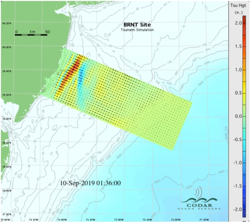
Figure 4.
Map of simulated heights/velocities for Brant Beach, New Jersey. In this map, the height of the wave is shown by color (see the color bar at the right), while the arrows represent particle (orbital) velocity. The largest vectors correspond to currents of ~1.0 m/s.
Figure 4.
Map of simulated heights/velocities for Brant Beach, New Jersey. In this map, the height of the wave is shown by color (see the color bar at the right), while the arrows represent particle (orbital) velocity. The largest vectors correspond to currents of ~1.0 m/s.
Figure 5.
BRNT simulated radial current velocities and the area-bands selected for the analysis which are 2 km wide and approximately parallel to the depth contours. The largest vectors correspond to currents of ~1.0 m/s.
Figure 5.
BRNT simulated radial current velocities and the area-bands selected for the analysis which are 2 km wide and approximately parallel to the depth contours. The largest vectors correspond to currents of ~1.0 m/s.
Figure 6.
Two-kilometer area-band velocity components VRef calculated from the simulated radials plotted versus time in hours. Distance offshore: blue 4–6 km; red 6–8 km; black 8–10 km; green 10–12 km; (a)/(b) velocity components perpendicular/parallel to the area-band boundary.
Figure 6.
Two-kilometer area-band velocity components VRef calculated from the simulated radials plotted versus time in hours. Distance offshore: blue 4–6 km; red 6–8 km; black 8–10 km; green 10–12 km; (a)/(b) velocity components perpendicular/parallel to the area-band boundary.
Figure 7.
Simulated velocities signaling the tsunami arrival. Area-band velocity components plotted versus time in hours: Distance offshore: blue 4–6 km; red 6–8 km; black 8–10 km; green 10–12 km; (a) velocity components perpendicular to the area-band boundary (b) velocity components parallel to the area-band boundary.
Figure 8.
Radar observations of 13 June 2013 band-velocities averaged over 12 min, plotted versus time (hours UTC from 13 June 2013, 17:09 meteotsunami): red 4–6 km; black 6–8 km; green 8–10 km; blue 10–12 km; maroon 12–14 km; yellow 14–16 km; cyan 16–18 km.
Figure 8.
Radar observations of 13 June 2013 band-velocities averaged over 12 min, plotted versus time (hours UTC from 13 June 2013, 17:09 meteotsunami): red 4–6 km; black 6–8 km; green 8–10 km; blue 10–12 km; maroon 12–14 km; yellow 14–16 km; cyan 16–18 km.
Figure 9.
Simulated tsunami heights averaged over area-bands. Distance offshore: blue 4–6 km; red 6–8 km; black 8–10 km; green 10–12 km.
Figure 9.
Simulated tsunami heights averaged over area-bands. Distance offshore: blue 4–6 km; red 6–8 km; black 8–10 km; green 10–12 km.
Figure 10.
Radial band velocities obtained every 2 min from measured BRNT radar cross spectra plotted vs. time (hours from May 30, 2019, 01:38 UTC) for bands: blue 2–4 km; red 4–6 km; black 6–8 km; green 8–10 km. (a)Velocity components perpendicular to the band boundary. (b) Velocity components are parallel to the band boundary.
Figure 11.
Radial area-band velocities and q-factors from combined BRNT CSQs for Fdetect = 0.5, plotted vs. time (hours from 30 May 2019, 01:38 UTC): (a) Velocity components perpendicular to the band boundary; blue 2–4 km; red 4–6 km; black 6–8 km; green 8–10 km; (b) Velocity components parallel to the band boundary; blue 2–4 km; red 4–6 km; black 6–8 km; green 8–10 km; (c) Perpendicular q-factors; blue 2–10 km; red 4–12 km; black 6–14 km; green 8–16 km. (d) Parallel q-factors; blue 2–10 km; red 4–12 km; black 6–14 km; green 8–16 km.
Figure 12.
Tsunami height required for detection plotted vs. date/time for bands: blue 2–4 km; red 4–6 km; black 6–8 km; green 8–10 km.
Figure 12.
Tsunami height required for detection plotted vs. date/time for bands: blue 2–4 km; red 4–6 km; black 6–8 km; green 8–10 km.
© 2019 by the authors. Licensee MDPI, Basel, Switzerland. This article is an open access article distributed under the terms and conditions of the Creative Commons Attribution (CC BY) license (http://creativecommons.org/licenses/by/4.0/).


