Article

Denoising Algorithm for the FY-4A GIIRS Based on Principal Component Analysis

1
Climate and Weather Disasters Collaborative Innovation Center, Key Laboratory for Aerosol-Cloud-Precipitation of China Meteorological Administration, School of Atmospheric Physics, Nanjing University of Information Science and Technology, Nanjing 210044, China
2
Numerical Weather Prediction Center of Chinese Meteorological Administration, Beijing 100081, China
3
National Meteorological Center, Beijing 100081, China
4
State Key Laboratory of Atmospheric Boundary Layer Physics and Atmospheric Chemistry, Institute of Atmospheric Physics, Chinese Academy of Sciences, Beijing 100029, China
*
Author to whom correspondence should be addressed.
Remote Sens. 2019, 11(22), 2710; https://doi.org/10.3390/rs11222710
Submission received: 27 August 2019 / Accepted: 14 November 2019 / Published: 19 November 2019
(This article belongs to the Special Issue Feature Papers for Section Atmosphere Remote Sensing)

Abstract

:
The Geostationary Interferometric Infrared Sounder (GIIRS) is the first high-spectral resolution advanced infrared (IR) sounder onboard the new-generation Chinese geostationary meteorological satellite FengYun-4A (FY-4A). The GIIRS has 1650 channels, and its spectrum ranges from 700 to 2250 cm−1 with an unapodized spectral resolution of 0.625 cm−1. It represents a significant breakthrough for measurements with high temporal, spatial and spectral resolutions worldwide. Many GIIRS channels have quite similar spectral signal characteristics that are highly correlated with each other in content and have a high degree of information redundancy. Therefore, this paper applies a principal component analysis (PCA)-based denoising algorithm (PDA) to study simulation data with different noise levels and observation data to reduce noise. The results show that the channel reconstruction using inter-channel spatial dependency and spectral similarity can reduce the noise in the observation brightness temperature (BT). A comparison of the BT observed by the GIIRS (O) with the BT simulated by the radiative transfer model (B) shows that a deviation occurs in the observation channel depending on the observation array. The results show that the array features of the reconstructed observation BT (rrO) depending on the observation array are weakened and the effect of the array position on the observations in the sub-center of the field of regard (FOR) are partially eliminated after the PDA procedure is applied. The high observation and simulation differences (O-B) in the sub-center of the FOR array notably reduced after the PDA procedure is implemented. The improvement of the high O-B is more distinct, and the low O-B becomes smoother. In each scan line, the standard deviation of the reconstructed background departures (rrO-B) is lower than that of the background departures (O-B). The observation error calculated by posterior estimation based on variational assimilation also verifies the efficiency of the PDA. The typhoon experiment also shows that among the 29 selected assimilation channels, the observation error of 65% of the channels was reduced as calculated by the triangle method.

Graphical Abstract

1. Introduction

In recent years, high-spectral resolution infrared (IR) sounders with thousands of channels have become a major part of the assimilation systems of many numerical weather prediction (NWP) centers and provide temperature and constituent profiles with a relatively high accuracy and vertical resolution [1].
Previous studies have reported that the assimilation of radiances from the advanced IR sounders (such as the Atmospheric Infrared Sounder (AIRS) onboard the Earth Observing System (EOS) Aqua platform [2], the Infrared Atmospheric Sounding Interferometer (IASI) onboard Europe’s Meteorological Operational (MetOp) satellites [3], and the Cross-Track Infrared Sounder (CrIS) onboard the Suomi National Polar orbiting Partnership and Joint Polar orbiting Satellite System series [4]) has a significant positive impact on global and regional NWPs [5,6,7,8,9,10]. The AIRS measures the radiance from Earth through 2378 channels covering a spectral interval from 650 to 2665 cm−1 at a resolution of approximately 1 cm−1. The AIRS is unique among these types of sounders because the instrument is a grating spectrometer rather than an interferometer. The IASI [11] is an IR Fourier transform spectrometer with 8461 channels covering the spectral interval from 645 to 2760 cm−1 at a resolution of 0.5 cm−1 (apodized). IASI radiances are currently assimilated operationally at several NWP centers [12,13,14]. The CrIS instrument is equivalent to the IASI on the National Polar Orbiting Operational Satellite System (NPOESS) series. The instrument has 1305 channels in the range of 650–2550 cm−1 and a spectral resolution between 1.125 and 4.5 cm−1 (Hamming-apodized).
The new-generation Chinese geostationary meteorological satellite FY-4A equipped with Geostationary Interferometric Infrared Sounder (GIIRS) was launched on 11 December 2016. The GIIRS is the first high-spectral-resolution advanced IR sounder onboard a geostationary weather satellite, unlike the AIRS, IASI and CrIS, which are in polar orbit [15]. The instrument has 1650 channels measuring the outgoing radiance with an unapodized spectral resolution of 0.625 cm−1 between 700 and 1130 cm−1 for the longwave band and between 1650 and 2250 cm−1 for the middlewave band, and the two bands have 689 and 961 channels, respectively. The longwave band is mainly designed for atmospheric temperature and ozone soundings, and the middlewave band is used primarily for atmospheric humidity sounding. The GIIRS has an unprecedented advantage in observing the fast-changing water vapor and temperature structures related to severe weather events [16,17]. FY-4A can provide vital information necessary for enhancing nowcasting and NWP services, for example, to improve local severe storm short-range forecasting via data assimilation [18].
However, a large number of IR hyperspectral channels operated by the GIIRS have very similar spectral signal characteristics and are highly correlated with each other in content, and a high degree of information redundancy occurs among these channels. Apart from these issues, noise also has an effect on the quality of observation data. Principal component analysis (PCA) is commonly used to reduce the dimensionality of a dataset with a large number of interdependent variables, and it is known as a multivariate analysis technique [19] and was first introduced by Pearson in 1901 and independently developed by Hotelling in 1933. The PCA has been used to detect and analyze the noise in satellite detection data for a long time. Recently, the approach has been applied to high-spectral resolution IR sounders [20]. PCA has been proven to be a valuable tool not only for compressing spectral data (in brightness temperature (BT) space) but also for smoothing out part of the instrument noise [21]. Huang and Antonelli [22] compressed high-spectral resolution IR data with PCA and achieved a substantial improvement of the signal-to-noise ratio by taking advantage of the redundancy present in the spectral domain. However, research has not used PCA to process GIIRS data.
This paper describes the implementation of a PCA-based denoising algorithm (PDA) and its application to simulated and observed data. We analyze the accuracy of the PDA by simulated data with different noise levels. Then, observations of GIIRS are used to reconstruct data and reduce noise by the PDA. This study focuses on (1) the application of the PDA method to reduce the noise present in hyperspectral IR observations, and (2) the reconstruction of the BT, which is linearly related to the characteristics of the original channel. The paper is organized as follows. The training, simulated and observed datasets and algorithms, including the model, instrument measurements and theoretical basis of the PDA, are described in Section 2. The main results and discussions are presented in Section 3. A summary and future research direction are given in Section 4.
Although most satellite IR measurements are likely to be cloud contaminated, a realistic simulation of the cloud effects is beyond the goal of this paper. Therefore, the results of the current study are applicable only to clear-sky observations.

2. Dataset and Algorithm

2.1. GIIRS Observations

GIIRS has 1650 spectral channels to obtain radiance in longwave infrared and middlewave infrared regions, which cover the spectral ranges of 700–1130 cm−1 (8.85–14.29 μm) and 1650–2250 cm−1 (4.44–6.06 μm) at a spectral interval of 0.625 cm−1. In this study, we only analyze the longwave infrared channels 1–128 (700–779.375 cm−1) shown in Figure 1a.
It takes 2.5 h for GIIRS to detect most of Chinese region (10°–60°N, 45°–165°E), including five rows, each of which requires 30 min and contains 84 fields of regard (FORs). Each FOR consists of a 32 × 4 array of squared fields of view (FOV). Each FOV corresponds to a specific detector and has a spatial horizontal resolution of around 16 km. Additionally, the Sensor Data Record (SDR) of GIIRS contains geolocated and calibrated radiance spectra converted from directly measured interferograms. For the unapodize SDR data, the Hamming apodization function with a three-point filter (0.23, 0.54 and 0.23) of running mean [23,24] is used. After the apodization, the BTs of the GIIRS channels are calculated from radiance data by Planck’s blackbody radiation law [24]. In this paper, we use the BTs [25]. The simulated dataset is the simulated BT obtained from the Radiative Transfer for TIROS Operational Vertical Sounder (RTTOV) model, and the observed dataset consists of the GIIRS observations.
Both a training dataset (including the simulated and observed datasets) and a testing dataset (GIIRS observations from March 15 to 31 and from September 12 to 15, 2018) of the longwave infrared channels 1–128 are applied. The single point observations are analyzed in Section 3.2.3 and the time-averages of all observation points are shown in Section 3.2.4 and afterwards. The GIIRS has advantages in observing the fast-changing vertical temperature and moisture structures of the atmosphere. The encrypted observations of the GIIRS from September 12 to 15, 2018 were recorded during super typhoon Mangkhut. Therefore, the observations are valuable and provide vital information for data assimilation.

2.2. Model Simulations

The Global/Regional Assimilation and Prediction System (GRAPES) is a new generation of numerical forecasting systems developed by the China Meteorological Administration [26]. The GRAPES Global/Regional Assimilation Forecasting System is a global/regional integration model that can be used as a GRAPES Global Forecasting System (GFS) global model or as a GRAPES regional mesoscale model [27]. In this study, the RTTOV version 9 is used as the forward radiative transfer model to perform the model simulations of the GIIRS BTs [28]. In addition, the National Centers for Environmental Prediction (NCEP) reanalysis data are used as the GRAPES-GFS background field to forecast 6 h without assimilation to obtain the forecast field. The 6-h forecast field of GRAPES-GFS at 0000, 0600, 1200 and 1800 UTC, a horizontal resolution of 0.25 × 0.25° and 62 vertical model levels is used as the background field. Then, the differences in BTs between the GIIRS observations and model simulations (O-B) are calculated by the GRAPES-GFS 4D-Var assimilation system, the time slot of GRAPES 4D-Var is 30 min in the 6-h assimilation time window.

2.3. Theoretical Basis of the PCA-Based Denoising Algorithm (PDA)

PCA is commonly used to reduce the dimensionality of a dataset with a large number of interdependent variables. This reduction is achieved by finding a set of Nt orthogonal vectors in the input space of dimension Nc, with Nt < Nc, which accounts for as much as possible of the data variance. Hence, the problem of dimensionality reduction is reduced to finding a linear transformation from the Nc-dimensional input space to the Nt-dimensional subspace spanned by the Nt orthogonal vectors defined above and hereinafter referred to as the principal components (PCs). The first PC is defined as the direction along which the variance in the input data reaches its maximum. The second PC is the vector in the orthogonal (Nt-1)-dimensional subspace that is complementary to the first PC, which explains most of the remaining variance and so on until the last PC is defined, which is the direction of the minimum variance [22].
PCA is also called eigenvector decomposition, and it is often used to approximate data vectors with many elements (e.g., the GIIRS observations of 1650 channels) by using a new set of data vectors with fewer elements, retaining most of the variability and information of the original data. The elements of a principal component score vector are projections of the spectrum onto each of the orthogonal basis vectors, which are the eigenvectors (the PCs) of the radiance covariance matrix. The total number of eigenvectors is equal to the total number of channels. However, a much smaller set of eigenvectors, k, ordered from largest to smallest eigenvalues, is sufficient to explain most of the variance in the original BT data.
If the original BT dataset is represented by m × n matrix Xmn (in our case, the centralized BT, which means BT after preprocessing), where m is the number of observations and n is the number of channels, then the covariance matrix, S, of the centralized BT is given by:
S = 1 n X T X
The matrix of eigenvectors V and Λ are related to covariance matrix S by:
S V = Λ V
where S, V and Λ are all dimensioned n × n , and Λ is a diagonal matrix of eigenvalues. Then, the k-th principal component of input vector X is the normalized eigenvector V k corresponding to eigenvalue λ k of covariance matrix S, where the eigenvalues are ordered λ 1 > λ 2 >…> λ k [29]. The first k PCs of V k (n × k) are obtained from the first k characters (usually k < n), and the dimensionality reduction dataset is computed as follows:
Y m k = X V k
Thereafter, the reconstructed dataset is computed by:
R m n = Y m k V k T
PCA and BT reconstruction are two techniques codefined as PDA, which can be used to compress the full spectrum from an IR sounding instrument with thousands of channels into a few hundred channels and reduce the noise.
In the simulation experiment, the simulated noisy BT (Bnoisy) with six different noise levels (a = 0.1, 0.5, 1.0, 1.5, 2.0, and 3.0) is defined in Equation (5) by:
n o i s e = a × 10 × N e D T × r a n d o m [ 1 , 1 ]
where NeDT (noise equivalent delta temperatures) is the noise level, which is extracted from the GIIRS observations in this paper and in the range 0–0.8 K. Then, the noisy BT can be expressed by Equation (6), below:
B n o i s y = B + n o i s e
where B represents the simulations. After PDA processing, Bnoisy becomes the reconstructed BT (R). The root-mean-square error of each channel is described by:
R M S E j = i = 1 m ( R B ) 2 m ( j = 1 , 2 , , n )
The noise level of each channel is then defined in Equation (8):
n o i s e l e v e l = j = 1 n R M S E j n
In the observation experiment, the reconstructed root-mean-square error of each channel is similar to Equation (7) and is calculated by the following equation and O means observations:
R M S E j = i = 1 m ( R O ) 2 m ( j = 1 , 2 , , n )

3. Results and Discussion

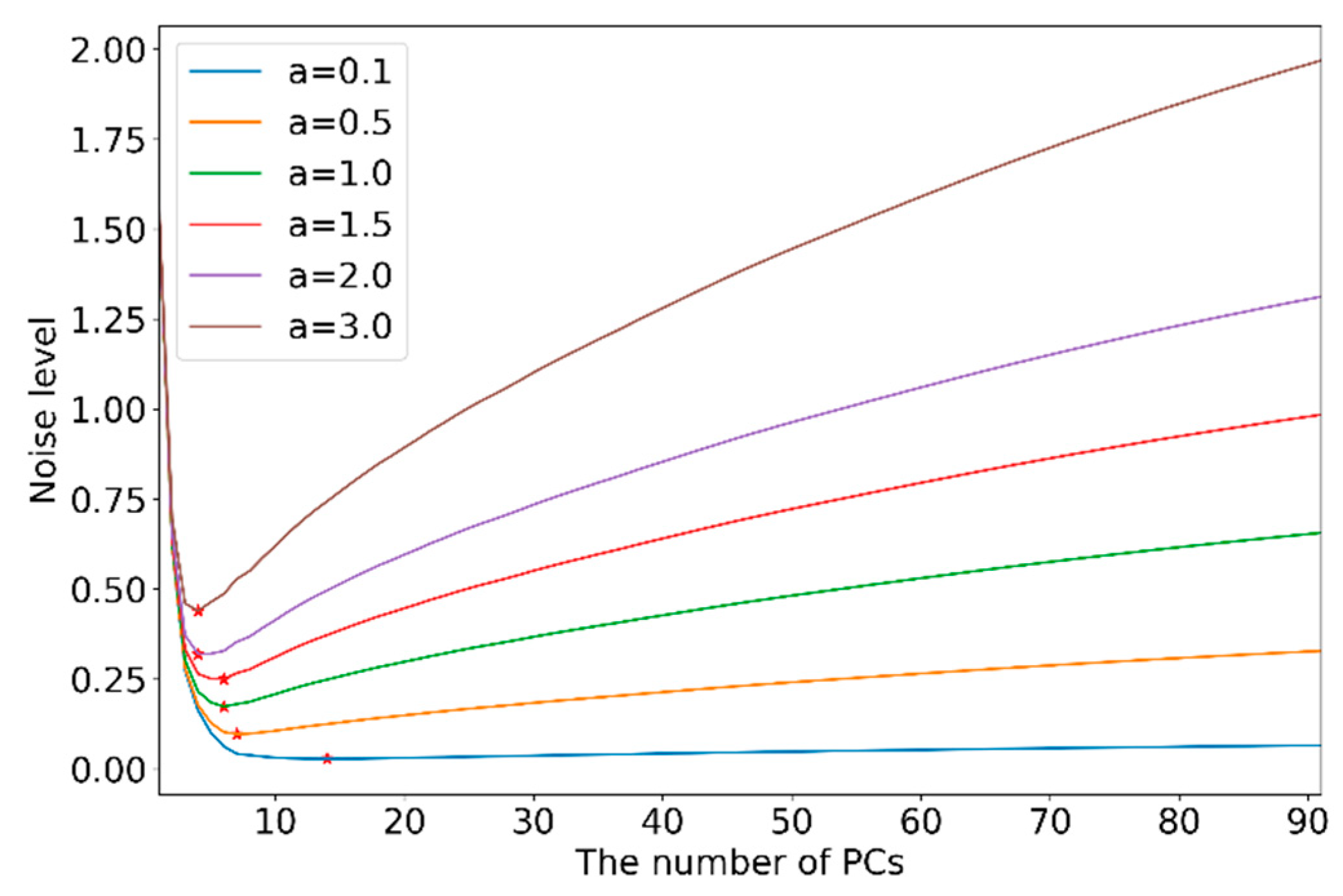
3.1. PDA Applied to Simulated Data

3.1.1. Simulation Dataset

A simulation experiment using a training dataset was designed to verify the denoising ability of the PDA, and the first 128 detection channels of the GIIRS-simulated BT were selected. Dataset A eliminated the contaminated channels for which the noise parameter (NeDT) > 0.15 K (channels 38–66) and the anomalous channels (channels 30–35 and 66–68) of the 128 channels. The dataset contained 24,645 profiles, ranging from 0000 to 0600 (UTC) on 30 January 2018. Figure 1 shows the simulated BT of the 128 original channels and 91 uncontaminated channels. The blue line represents the mean value of the BT, and the red short lines represent the standard deviation, which indicates the fluctuation range of the BT. The first 128 sounding channels can cover the spectrum for most of the atmospheric molecule detection from the near surface to the atmospheric window.

3.1.2. PDA Performance on Simulated Data

The simulated BT dataset with different noise levels was designed to evaluate the performance of the PDA. First, the observed NeDT was used to simulate different noise levels. The simulated noise was multiplied by a random disturbance and noise figure based on the observed noise. Six values of the noise figure (i.e., a value) were used in this experiment, namely, 0.1, 0.5, 1.0, 1.5, 2.0, and 3.0. Then, the radiative transfer model was used to simulate the noisy BT (Bnoisy) with the six noise levels, and the PDA was applied to the Bnoisy dataset.
The relationship between the optimum number of PCs and the noise level is shown in Figure 2. When the noise level reached a minimum, the number of PCs was considered to be the optimum number of PCs. As the noise increased, the required number of PCs decreased. The optimum number of PCs for the six cases with a values of 0.1, 0.5, 1.0, 1.5, 2.0, and 3.0 were 14, 7, 6, 6, 4, and 4, respectively.

3.2. PDA Applied to Observed Data

This section describes the application of the PDA to the observations collected by the GIIRS in different time ranges and shows the impact of the PDA on the observations. The performance of the PDA was evaluated by comparing the simulated BT with the observed BT by the GIIRS. The variational assimilation requires both the observation error and the background error to follow an unbiased Gaussian distribution. However, observations (O) and simulations (B) always have errors (called μ o and μ b , respectively). It is important for data assimilation to remove these biases [30]. The statistical expectation value of observations minus simulations differences (O-B) is related to μ o and μ b as shown in Equation (10). Therefore, it is critical to evaluate the bias characteristics of the O-B (O-B) and reconstructed O-B (rrO-B) in the following.
O B ¯ = ( T + μ 0 ) ( T + μ b ) ¯ = μ 0 + μ b ¯

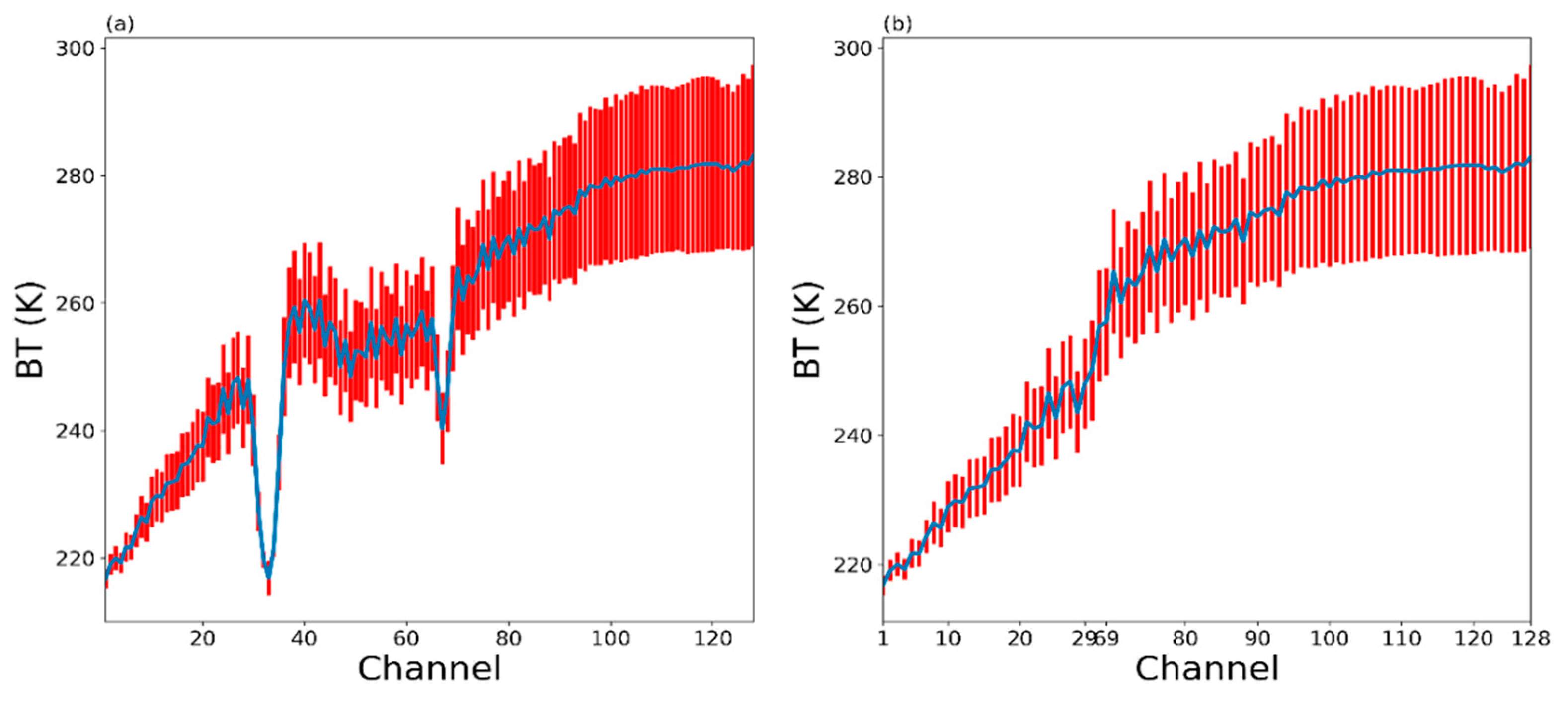
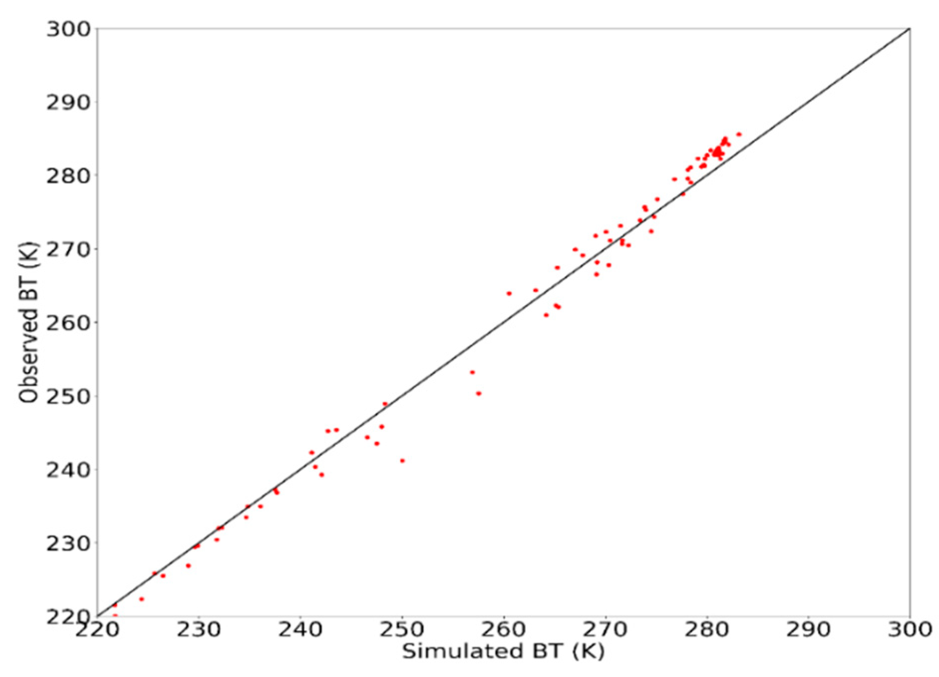
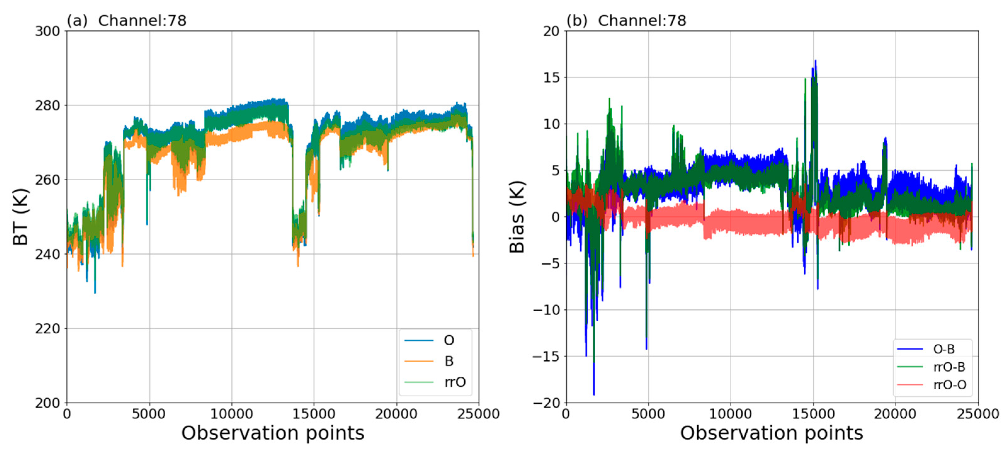
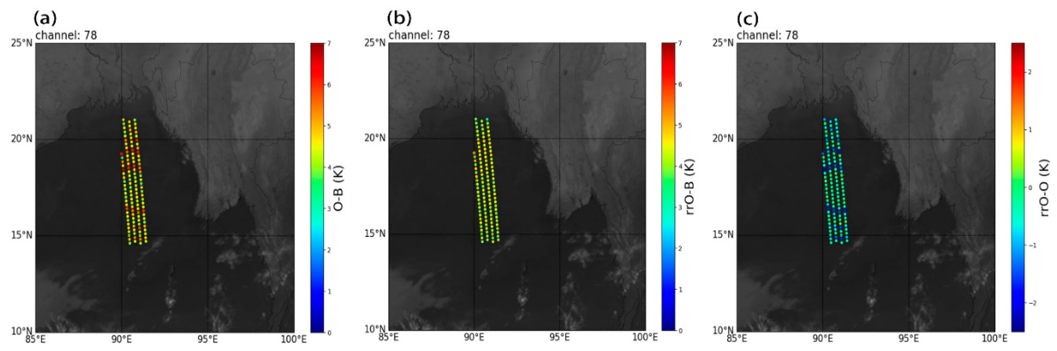
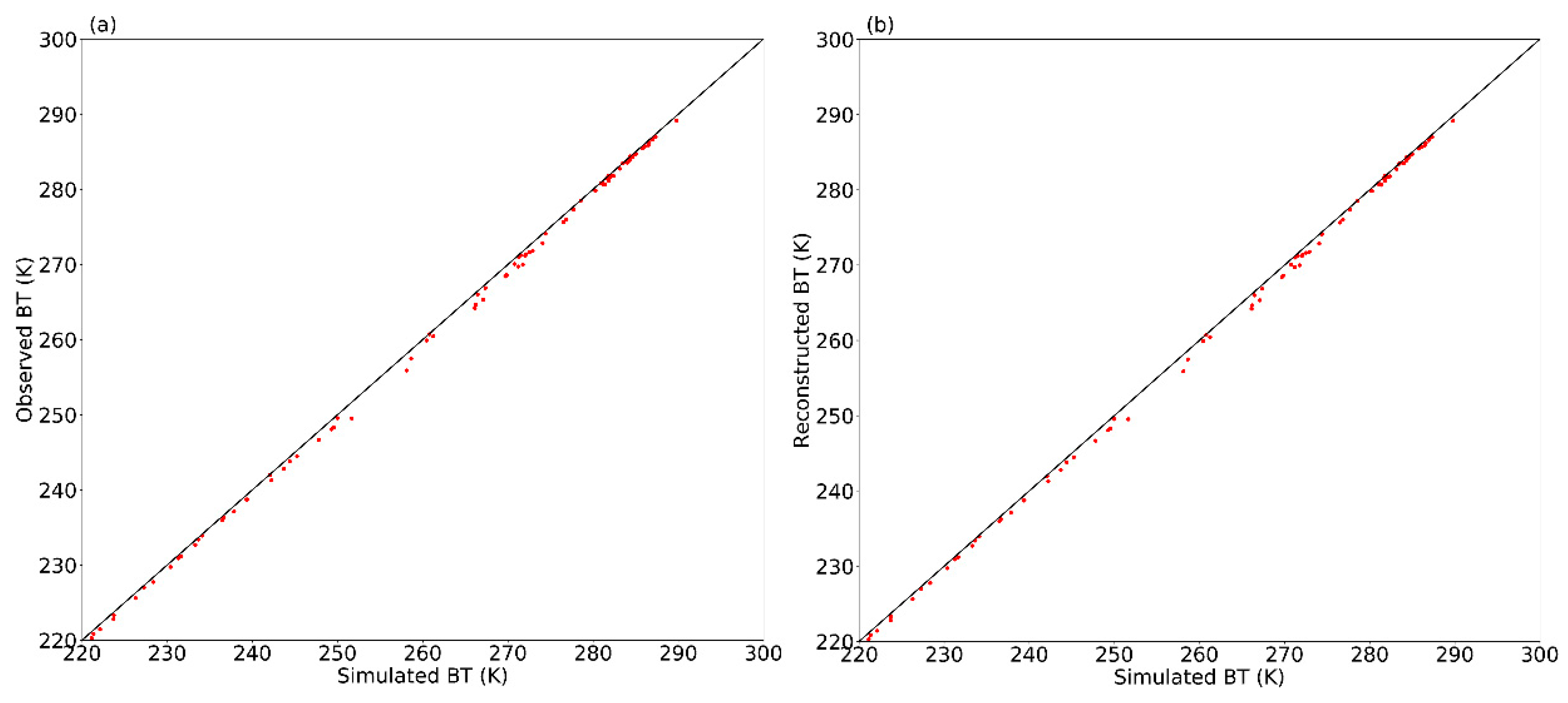
3.2.1. Original Observed and Simulated BT Data

The simulation experiment achieved the desired results, and then we use the observations to analyze the denoising performance of the PDA. As shown in Figure 3, the values of observed BT and simulated BT are between 220 to 285 K, and most dots are distributed near the 1:1 line.

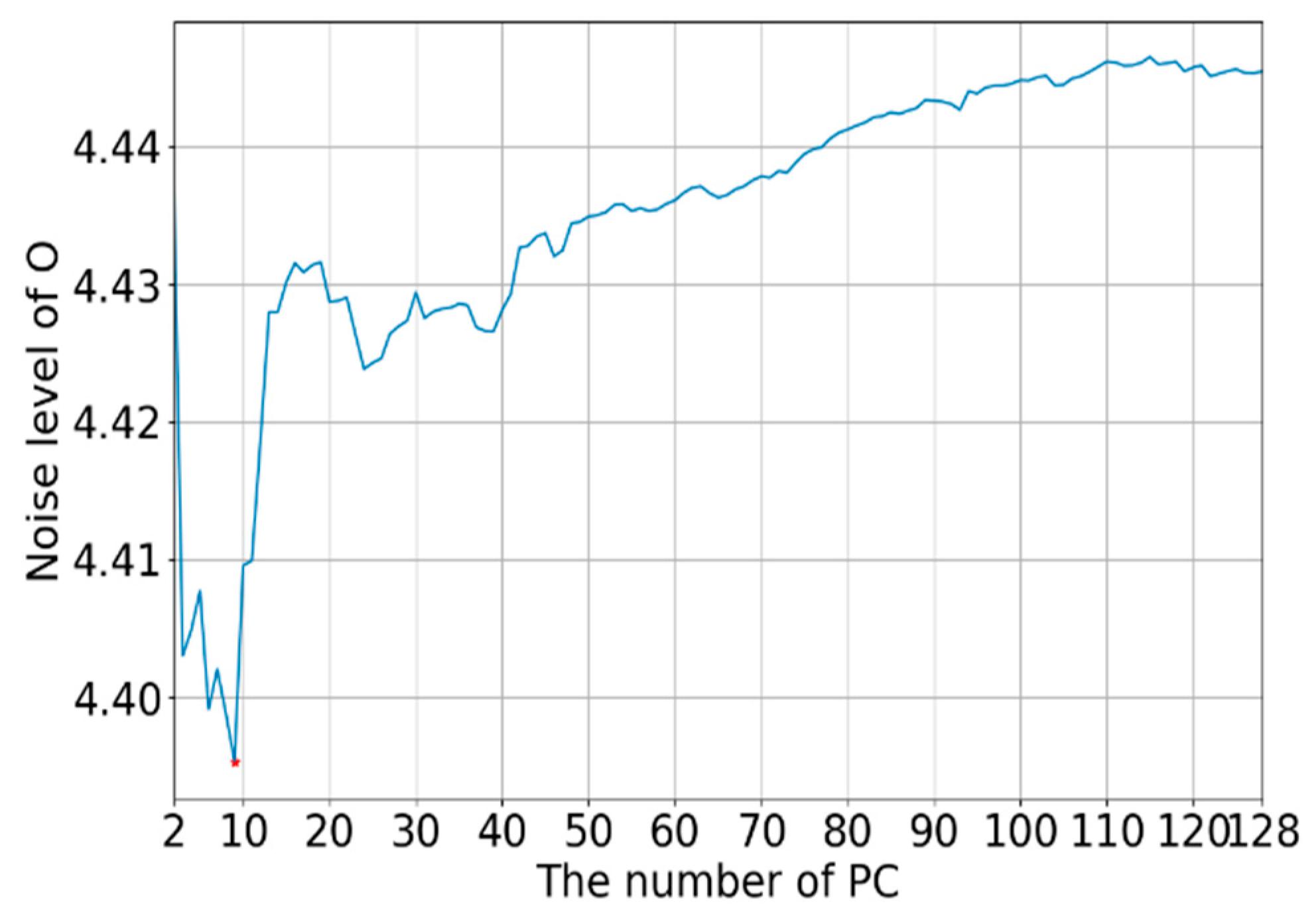
3.2.2. Method for Selecting the Optimal Number of PCs

When dealing with real data, the first step is to determine the optimal number of PCs. Therefore, we introduced an approach based on the minimization of the noise level function, as defined in Equation (8).
Similar to the simulation experiment, the noise level of the observation data reached a minimum when there were 9 PCs (shown in Figure 4). As a result, we chose the first nine PCs for reconstruction in this observation experiment. The eigenvalues generated from the clear-sky GIIRS observations (not shown here) show that nearly 100% of the variance is explained with only the first nine PCs. A widely accepted method for determining the optimal number of PCs, Nt, requires the ratio of the variance explained by the first Nt PCs and the total data variance to be close to 1 [19]. Here, the ratio of the variance explained by the first nine PCs to the total data variance is larger than 0.999, which ensures that the retained PCs explain most of the raw signal variance. Instead of using all channels, only 9 PCs are needed to reconstruct the BT. As a data compression technology, PCA is more efficient.

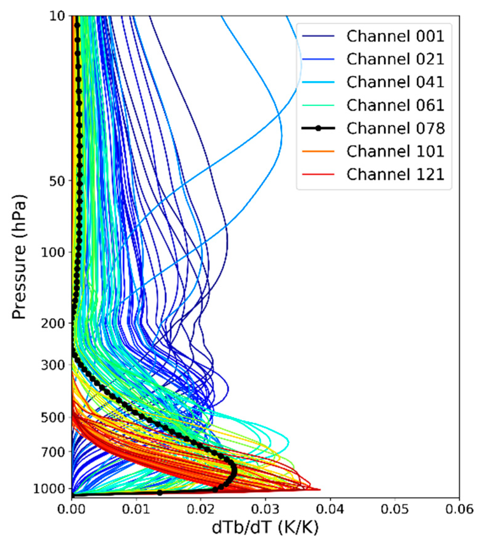
3.2.3. Selection of the Representative Channels

Jacobians indicate the sensitivities of the BT obtained by the satellite associated with changes in atmospheric parameters, such as the air temperature, water vapor content, and ozone level. The Jacobians of the temperature, water vapor content, and ozone level are defined as dBT/dT, dBT/dlog(Q), and dBT/dlog(O3), respectively, where T, Q, and O3 are the profiles of the air temperature (in kelvins), water vapor mixing ratio (in grams per kilogram), and ozone level (in parts per million by volume), respectively. Figure 5 shows the vertical distribution of the temperature Jacobian function for 91 uncontaminated channels in bands of GIIRS longwave IR channel. The temperature vertical information in the troposphere can be derived mainly from the longwave IR channels. Channel 78 represents the atmospheric information at approximately 850 hPa (the middle layer of the troposphere), which is selected to verify the effect of the PDA.
The observed, simulated and reconstructed BT values at all observation points of channel 78 are shown in Figure 6a. The reconstructed BT is closer to the simulated BT than the observed BT. The O-B, rrO-B, and reconstructed observation departures (rrO-O) at all observation points of channel 78 are shown in Figure 6b. The reconstructed observation departures are small, fluctuating around zero. After PDA processing, the reconstructed background departures are smaller than the original background departures.
The array distribution characteristics of the O-B, rrO-B, and rrO-O of channel 78 are shown in Figure 7. The difference of O-B in different FOVs is notable in Figure 7a. In the center of the observation array, the O-B are smaller than those in the sub-center. On both sides of the sub-center area of the observation array, the O-B are apparently larger, especially in the 9th, 20th, 24th, 27th (1st –32nd), 41st, 53rd, 57th, 62nd (33rd–64th), 73rd, 84th, 88th, 91st (65th–96th), 106th, 116th and 120th (97th–128th) FOVs, O-B are larger than 5 k. After PDA reconstruction processing, the rrO-B are smaller and smoother than before, and the reconstructed BT is closer to the simulated BT. In those sub-center FOVs, the reduction of O-B is greater than 1 k. The main change caused by the PDA process is in the sub-center area of the observation array. The probability distribution function (PDF) of the O-B before and after reconstruction is shown in Figure 8. The skewness basically remains unchanged, and the kurtosis is larger after PDA reconstruction processing. A larger kurtosis coefficient indicates a more concentrated data distribution.

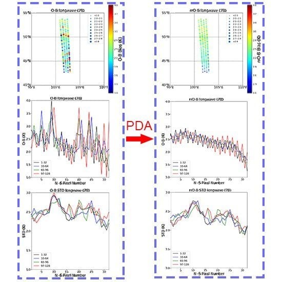
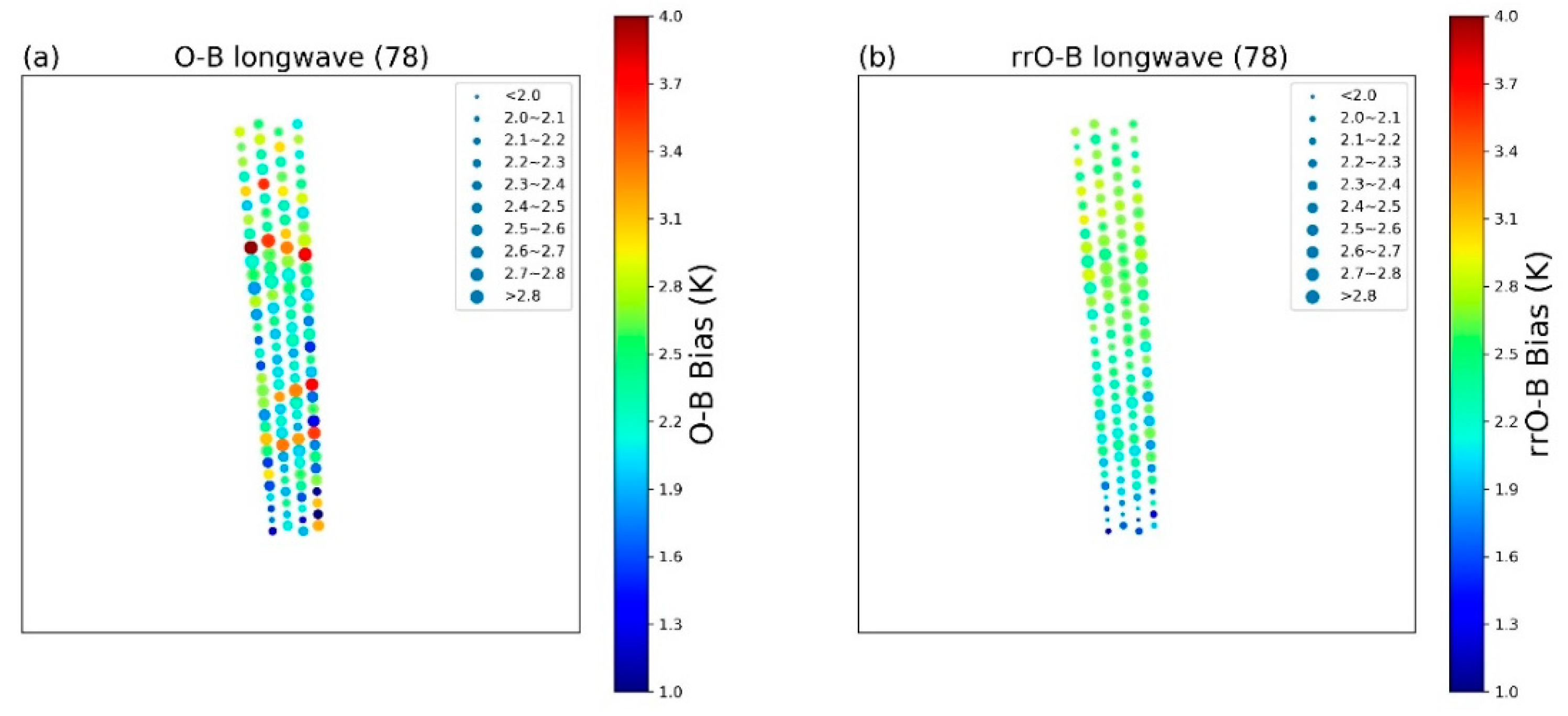
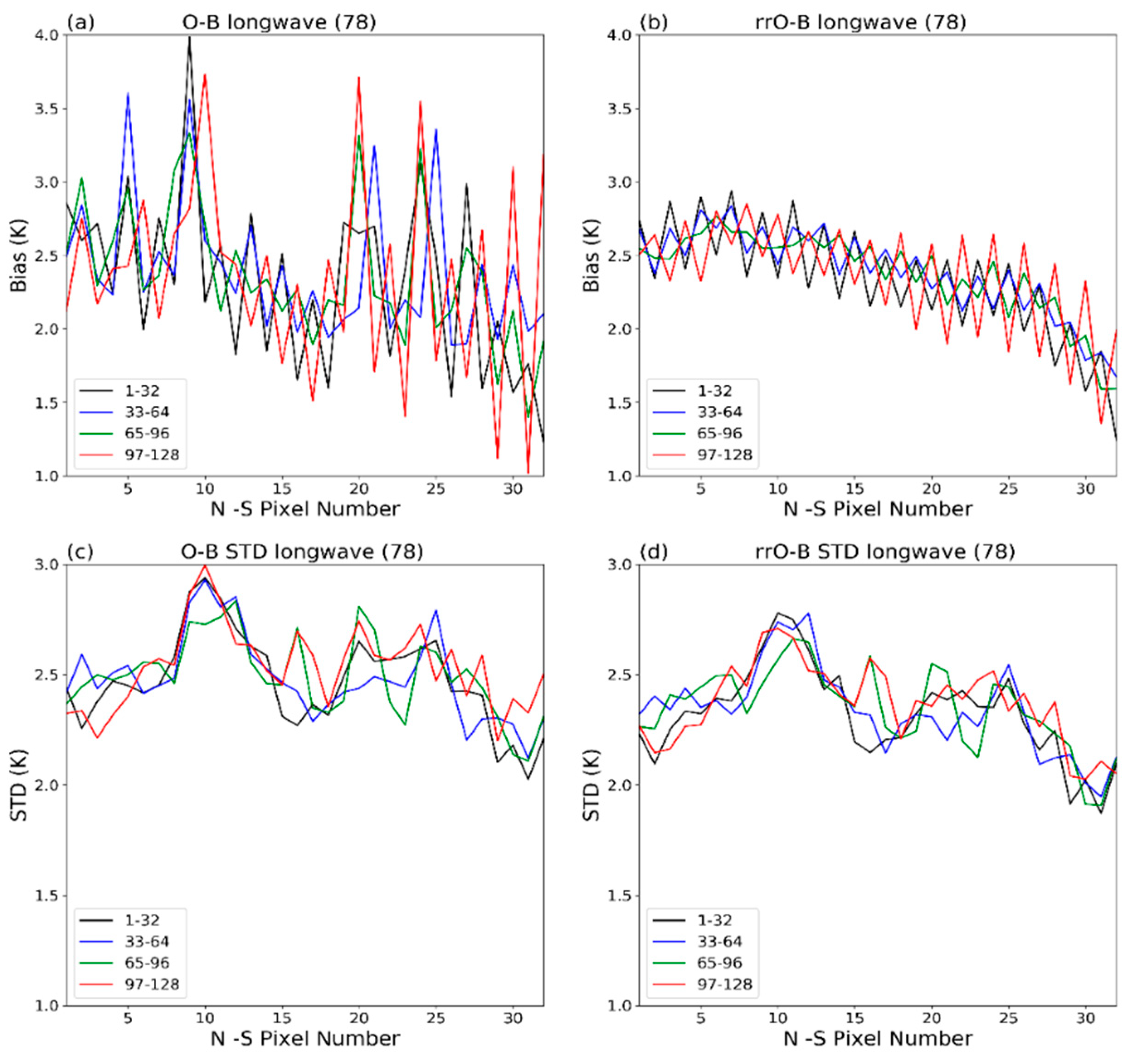
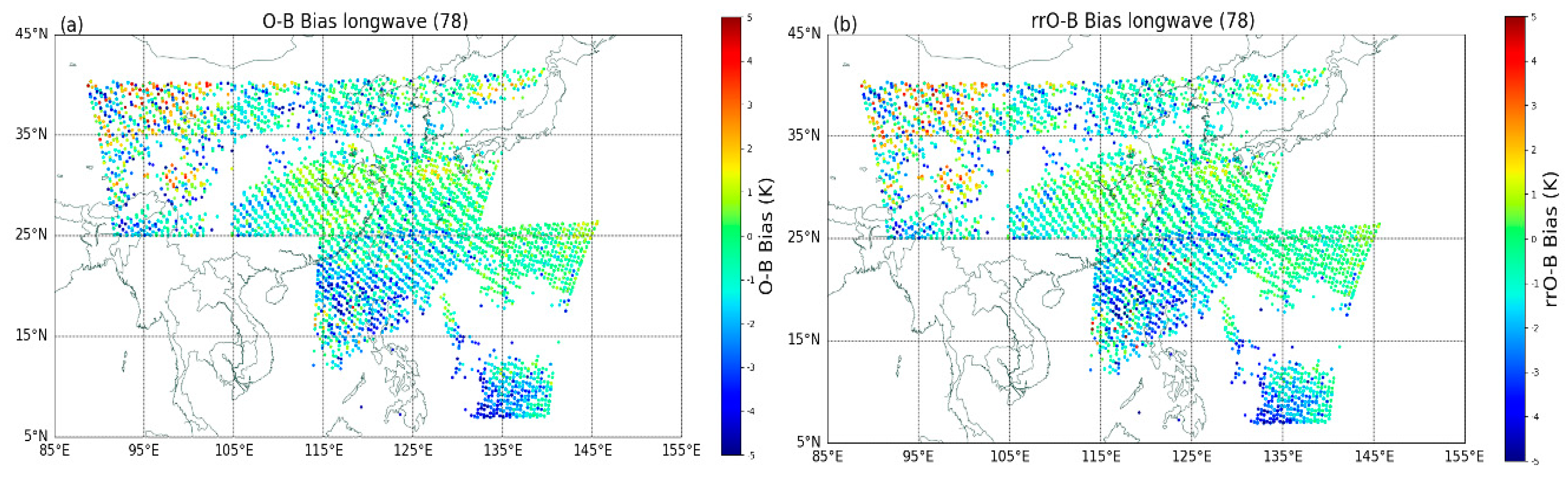
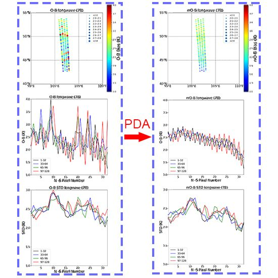
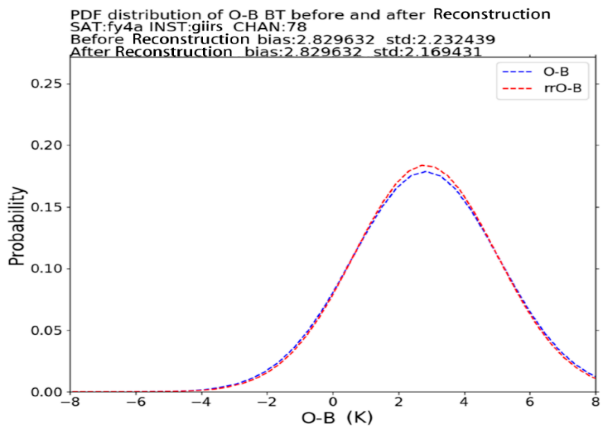
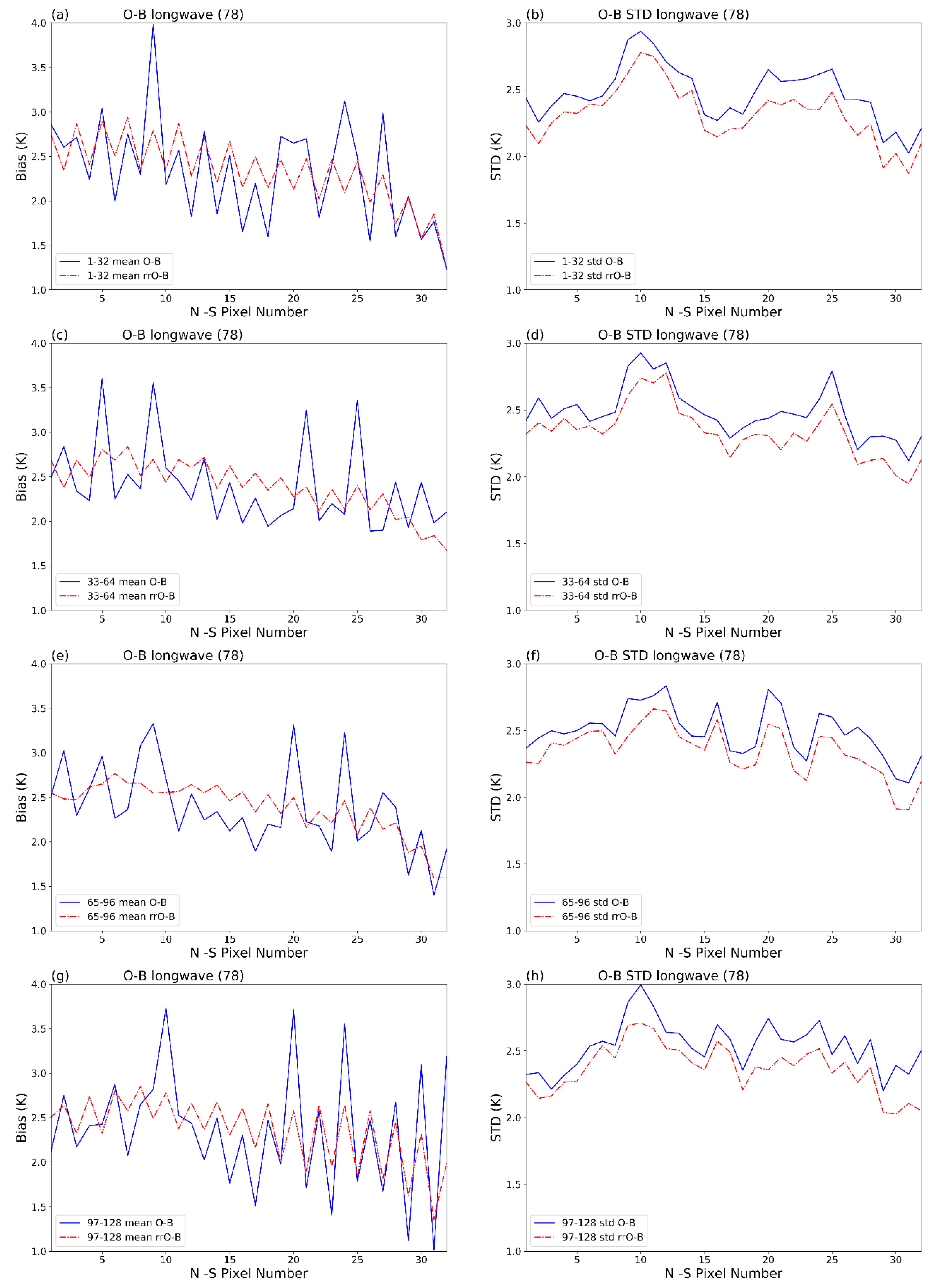
3.2.4. Statistics of the Half-Month Average Background Departures

A testing dataset of GIIRS observations from March 15 to March 31, 2018, of the 91 uncontaminated (the same as dataset A in Section 3.1.1) IR longwave temperature channels were selected to conduct statistical analysis. The half-month average array distribution characteristics of the O-B and rrO-B are shown in Figure 9. The difference of O-B in different FOVs is notable in Figure 9a. In the center of the observation array, the O-B are smaller than those in the sub-center. On both sides of the sub-center area of the observation array, the O-B are apparently larger, especially in the 9th, 24th (1st–32nd), 37th, 41st, 53rd, 57th (33rd–64th), 73rd, 84th, 88th (65th –96th), 106th, 116th and 120th (97th–128th) FOVs, and the O-B are larger than 3 k. After reconstruction by the PDA method, the rrO-B become smoother as a whole and the standard deviation is slightly lower than before as shown in Figure 9b. In those sub-center FOVs, the O-B reduction is greater than 0.8 k. The main change caused by the PDA process is in the sub-center area of the observation array. The results show that the array features are weakened and the effect of the array position on the observations is partially eliminated after applying the PDA procedure.
From another perspective, the original and reconstructed background departures and the standard deviations of the original and reconstructed background departures of channel 78 with the number of detection pixels are shown in Figure 10. The sawtooth shape is more visible and smoother after the PDA procedure is applied. The improvement of the high O-B bias is more notable, and the low O-B bias becomes smoother. The O-B and rrO-B of channel 78 changes in the range of 1st to 32nd FOVs, 33rd to 64th FOVs, 65th to 96th FOVs, and 97th to 128th FOVs are shown in Figure 11a,c,e,g, respectively. The high O-B bias in the sub-center of the field of regard (FOR) array notably reduced. The standard deviations of the O-B and the rrO-B of channel 78 in the ranges of 1st to 32nd FOVs, 33rd to 64th FOVs, 65th to 96th FOVs, and 97th to 128th FOVs are shown in Figure 11b,d,f,h, respectively. In each scan line, the standard deviation of the rrO-B is lower than that of the O-B.

3.2.5. Assimilation Experiment

To evaluate the reconstruction effect, three parallel data assimilation experiments are carried out. The first assimilation experiment is the control experiment, which is consistent with the GRAPES operational assimilation system. Conventional observations, satellite observations of the AMSU-A, ATMS, and AIRS and GPS RO, scatwind, and Gpspw data from the instruments mounted on the NOAA-15, NOAA-18, NOAA-19, Metop-A, and Metop-B satellites are included in the assimilation data. The second assimilation experiment involves the GIIRS-observed BT data. The observed BT of the GIIRS temperature detection channel (sparse to 200 km) is compared with that of the control experiment. The third assimilation experiment involves the GIIRS-reconstructed BT data. Compared with the control experiment, the reconstructed BT of the GIIRS temperature detection channel (sparse to 200 km) is added. The time period of the three assimilation experiments is ten days (0000 UTC 1 March to 0000 UTC 11 March 2018).
Quality control before data assimilation is needed, including channel selection, anomalous value culling, cloud detection, and deviation correction. Optimal channel selection is key for variational assimilation and inversion of the hyperspectral atmospheric vertical detectors. Optimal channel selection can reduce the variational assimilation and inversion ill-posedness caused by the observed redundant information from hyperspectral detectors, and further solve the channel dimensionality disaster problem [31]. Anomalous value culling uses the dual weight method [32]. In this study, the cloud mask (CLM) of the Advanced Geostationary Radiation Imager (AGRI) onboard the FY-4A geostationary meteorological satellite, is used to determine whether the FOV of the GIIRS is subject to cloud coverage. The horizontal resolution of the AGRI CLM is 4 km, and the spatial resolution of the GIIRS is 16km. Therefore, the cloud information of the 16 pixels of the AGRI CLM is considered to be in the GIIRS FOV. The cloud information in CLM is divided into four categories: cloudy, possibly cloudy, possibly clear sky and clear sky. Finally, 16 adjacent clear-sky pixels were selected as the GIIRS FOV corresponding to clear-sky conditions. Variational assimilation requires that the O-B of the channel BT satisfies the Gaussian distribution. The radiation transmission mode itself contains errors, and the fundamental spectral data of the radiation transmission mode as well as the input data (temperature, humidity profile, etc.) also contain errors. The satellite observation data also contain errors due to the influences of instrument sensitivity and calibration. Therefore, before assimilation of the satellite-observed BT, deviation correction must be performed to correct or reduce the above error so that the corrected O-B data satisfy the Gaussian distribution. The array deviation correction calculated from the half-month average is used in this work.
After assimilation, posterior estimation based on variational assimilation [33], also known as the triangle method, is applied to calculate the observation error (shown in Table 1). The observation error reduction ratio is defined in Equation (11) by
R a t i o   =   ( E E r r ) / E
The effect of reconstruction is measured and evaluated by the observation error reduction ratio. Among the 29 selected assimilation channels, the observation error of 72.4% of the channels reduced as calculated by the triangle method. In particular, the observation error of some channels, such as channels 73, 80, and 90, exhibit a notable reduction, and the observation error reduction ratios are 18.11%, 13.63% and 16.57%, respectively.

3.2.6. Typhoon Experiment

The GIIRS has an unprecedented advantage in observing the fast-changing vertical temperature and moisture structures of the atmosphere related to severe weather events, such as typhoons. The encrypted observations of the GIIRS from September 12 to 15, 2018 of super typhoon Mangkhut hitting mainland China, lashing Hong Kong, and causing dozens of casualties in the Philippines are valuable. The observations provide vital information necessary for improving local severe storm short-range forecasts via data assimilation.
The spatial distribution characteristics of the O-B and rrO-B of channel 78 during typhoon Mangkhut are shown in Figure 12. The departures are in the range of −5 K to 5 K, and the values during the typhoon are mainly less than 0. The differences of O-B and rrO-B distribution characteristics are small, and the main difference is in the southeast coastal area and Yellow Sea. Figure 13 compares observed BT with the simulated BT and the reconstructed BT against the simulated BT all channels’ average during typhoon Mangkhut. Overall, the observed BT values and reconstructed BT values are all below the 1:1 line and a significant change from the 1:1 line is not observed. However, the average array distribution characteristics of the O-B and rrO-B during typhoon Mangkhut are clear in Figure 14. After reconstruction by the PDA method, the array features are weakened and the effect of the array position on the observations is partially eliminated, which is consistent with the results obtained in Section 3.2.4.
The parallel data assimilation experiments of typhoon Mangkhut are carried out as described in Section 3.2.5. The observation errors during typhoon Mangkhut calculated by posterior estimation based on variational assimilation are summarized in Table 2. Among the 29 selected assimilation channels, the observation error of 65% of the channels is reduced based on the triangle method. In particular, the observation error of some channels, such as channels 78, 86, 91 and 113, exhibit a clear reduction, and the observation error reduction ratios are 3.18%, 3.55%, 4.05%, and 3.42%, respectively.

4. Summary

We have assessed the performance of the PDA, a technique largely applied to data noise reduction problems, on high-spectral resolution IR measurements observed by the GIIRS. The purpose of the study is to reduce the random and array-dependent components of the instrument noise to allow for more accurate retrievals of atmospheric parameters and for more accurate validations of the radiative transfer model.
Both simulated data and observations were used to better understand the effects of the PDA on the data and to partially prove the robustness of the algorithm. The results demonstrate that the PDA is effective in processing the large volume of data provided by the new generation of instruments and is an efficient method of reducing noise in the observations.
A simulation experiment was conducted to demonstrate the application of the PDA to simulated BT data with different noise levels. The results show that as the noise increases, the optimum number of required PCs decreases. When the noise figure has values of a = 0.1, 0.5, 1.0, 1.5, 2.0, and 3.0, the optimum numbers of PCs for the 91 uncontaminated channels are 14, 7, 6, 6, 4, and 4, respectively. Channel 78 is selected as a representative channel in the observation experiment. The noise level of the observation data reaches a minimum at 9 PCs. As a result, we select the first nine PCs for reconstruction in the observation experiment in this study. The reconstructed BT is closer to the simulated BT than the observed BT. Compared with the O-B, the reconstructed background departures are smaller and smoother than before, especially on both sides of the sub-center of the FOR. The reconstructed observation departures are small and fluctuate around zero. The results of the half-month average O-B and rrO-B further show that the array features are weakened and the effect of the array position on the observations is partially eliminated after the PDA procedure is applied. The high O-B bias in the sub-center of the FOR array are notably reduced, and the sawtooth shape of the O-B with the number of detection pixels becomes more visible and smoother after the PDA procedure is applied. In each scan line, the standard deviation of the rrO-B is lower than that of the O-B. Posterior estimation based on variational assimilation of the assimilation experiment is applied to calculate the observation error. Both the assimilation and typhoon experiments show that the observation error has reduced as calculated by the triangle method.
The techniques used in this study are valuable tools for data compression, noise reduction and data reconstruction and will be helpful for the accurate retrieval of meteorological parameters from new-generation satellite instruments.

Author Contributions

Conceptualization, S.F. and W.H.; methodology, S.F. and W.H.; validation, Z.G. and W.H.; formal analysis, S.F., R.Y. and Y.Z.; resources, W.H. and Z.G.; data curation, S.F.; writing—original draft preparation, F.S.; writing—review and editing, W.H., Z.G., R.Y. and Y.Z.

Funding

This research was funded by the National Natural Science Foundation of China under Grant 41675108, the National Key Laboratory of Science and Technology on Space Microwave under grant 2018SSFNKLSMT-14t and the National key research and development program (2018YFC1506700).

Acknowledgments

The first author is very grateful to Bing Tong for his helpful comments.

Conflicts of Interest

The authors declare no conflict of interest.

References

  1. Menzel, W.P.; Schmit, T.J.; Zhang, P.; Li, J. Satellite-based atmospheric infrared sounder development and applications. Bull. Am. Meteorol. Soc. 2018, 99, 583–603. [Google Scholar] [CrossRef]
  2. Chahine, M.T.; Pagano, T.S.; Aumann, H.H.; Atlas, R.; Barnet, C.; Blaisdell, J.; Chen, L.; Divakarla, M.; Fetzer, E.J.; Goldberg, M.; et al. AIRS: Improving weather forecasting and providing new data on greenhouse gases. Bull. Am. Meteorol. Soc. 2006, 87, 911–926. [Google Scholar] [CrossRef]
  3. Hilton, F.; Armante, R.; August, T.; Barnet, C.; Bouchard, A.; Camy-Peyret, C.; Capelle, V.; Clarisse, L.; Clerbaux, C.; Coheur, P.-F.; et al. Hyperspectral earth observation from IASA: Five years of accomplishments. Bull. Am. Meteorol. Soc. 2012, 93, 347–370. [Google Scholar] [CrossRef]
  4. Goldberg, M.D.; Kilcoyne, H.; Cikanek, H.; Mehta, A. Joint polar satellite system the United States next generation civilian polar-orbiting environment satellite system. J. Geophys. Res. Atmos. 2013, 118, 13463–13475. [Google Scholar] [CrossRef]
  5. Le Marshall, J.; Jung, J.; Derber, J.; Chahine, M.; Treadon, R.; Lord, S.J.; Goldberg, M.; Wolf, W.; Liu, H.C.; Joiner, J.; et al. Improving global analysis and forecasting with AIRS. Bull. Am. Meteorol. Soc. 2006, 87, 891–895. [Google Scholar] [CrossRef]
  6. Li, J.; Wang, P.; Han, H.; Li, J.L.; Zheng, J. On the assimilation of satellite sounder data in cloudy skies in the numerical weather prediction models. J. Meteorol. Res. 2016, 30, 169–182. [Google Scholar] [CrossRef]
  7. McNally, T.; Bonavita, M.; Thépaut, J.-N. The role of satellite data in the forecasting of Hurricane Sandy. Mon. Weather Rev. 2014, 142, 634–646. [Google Scholar] [CrossRef]
  8. Wang, P.; Li, J.; Li, J.L.; Li, Z.L.; Schmit, T.J.; Bai, W.G. Advanced infrared sounder subpixel cloud detection with imagers and its impact on radiance assimilation in NWP. Geophys. Res. Lett. 2014, 41, 1773–1780. [Google Scholar] [CrossRef]
  9. Wang, P.; Li, J.; Goldberg, M.D.; Schmit, T.J.; Lim, A.H.N.; Li, Z.L.; Han, H.; Li, J.L.; Ackerman, S.A. Assimilation of thermodynamic information from advanced infrared sounders under partially cloudy skies for regional NWP. J. Geophys. Res. Atmos. 2015, 120, 5469–5484. [Google Scholar] [CrossRef]
  10. Wang, P.; Li, J.; Li, Z.L.; Lim, A.H.N.; Li, J.L.; Schmit, T.J.; Goldberg, M.D. The impact of Cross-track Infrared Sounder (CrIS) Cloud Cleared Radiances on Hurricane Joaquin (2015) and Matthew (2016) Forecasts. J. Geophys. Res. Atmos. 2017, 122, 13201–13218. [Google Scholar] [CrossRef]
  11. Chalon, G.; Cayla, F.; Diebel, D. IASI—An advanced sounder for operational meteorology. In Proceedings of the IAF 52nd International Astronautical Congress, Toulouse, France, 1–5 October 2001. [Google Scholar]
  12. Hilton, F.; Atkinson, N.C.; English, S.J.; Eyre, J.R. Assimilation of IASI at the Met Office and assessment of its impact through observing system experiments. Q. J. R. Meteorol. Soc. 2009, 135, 495–505. [Google Scholar] [CrossRef]
  13. Hilton, F.; Collard, A.; Guidard, V.; Randriamampianina, R.; Schwaerz, M. Assimilation of IASI radiances at European NWP centres. In Proceedings of the Workshop on the assimilation of IASI data in NWP, ECMWF, Reading, UK, 6–8 May 2009; pp. 6–8. [Google Scholar]
  14. Collard, A.D.; McNally, A.P. The assimilation of Infrared Atmospheric Sounding Interferometer radiances at ECMWF. Q. J. R. Meteorol. Soc. 2009, 135, 1044–1058. [Google Scholar] [CrossRef]
  15. Yang, J.; Zhang, Z.Q.; Wei, C.Y.; Lu, F.; Guo, Q. Introducing the new generation of Chinese geostationary weather satellites, FengYun-4. Bull. Am. Meteorol. Soc. 2017, 98, 1637–1658. [Google Scholar] [CrossRef]
  16. Li, J.; Li, J.L.; Otkin, J.; Schmit, T.J.; Liu, C.-Y. Warning information in a preconvection environment from the geostationary advanced infrared sounding system—A simulation study using IHOP case. J. Appl. Meteorol. Clim. 2011, 50, 776–783. [Google Scholar] [CrossRef]
  17. Li, J.; Liu, C.-Y.; Zhang, P.; Schmit, T.J. Applications of full spatial resolution space-based advanced infrared soundings in the preconvection environment. Weather Forecast. 2012, 27, 515–524. [Google Scholar] [CrossRef]
  18. Li, Z.L.; Li, J.; Wang, P.; Lim, A.; Li, J.L.; Schmit, T.J.; Atlas, R.; Boukabara, S.-A.; Hoffman, R.N. Value-added impact of geostationary hyperspectral infrared sounders on local severe storm forecasts-via a quick regional OSSE. Adv. Atmos. Sci. 2018, 35, 1217–1230. [Google Scholar] [CrossRef]
  19. Jolliffe, I.T. Principal Component Analysis; Springer: Berlin/Heidelberg, Germany, 1986. [Google Scholar]
  20. Collard, A.D.; McNally, A.P.; Hilton, F.I.; Healy, S.B.; Atkinson, N.C. The use of principal component analysis for the assimilation of high-resolution infrared sounder observations for numerical weather prediction. Q. J. R. Meteorol. Soc. 2010, 136, 2038–2050. [Google Scholar] [CrossRef]
  21. Antonelli, P.; Revercomb, H.E.; Sromovsky, L.A. A principal component noise filter for high spectral resolution infrared measurements. J. Geophys. Res. Atmos. 2004, 109. [Google Scholar] [CrossRef]
  22. Huang, H.-L.; Antonelli, P. Application of principal component analysis to high-resolution infrared measurement compression and retrieval. J. Appl. Meteorol. 2001, 40, 365–388. [Google Scholar] [CrossRef]
  23. Han, Y.; Revercomb, H.; Cromp, M.; Gu, D.G.; Johnson, D.; Mooney, D.; Scott, D.; Strow, L.; Bingham, G.; Borg, L. Suomi NPP CrIS measurements, sensor data record algorithm, calibration and validation activities, and record data quality. J. Geophys. Res. Atmos. 2013, 118, 12734–12748. [Google Scholar] [CrossRef]
  24. Li, X.; Zou, X.L. Bias characterization of CrIS radiances at 399 selected channels with respect to NWP model simulations. Atmos. Res. 2017, 196, 164–181. [Google Scholar] [CrossRef]
  25. Yin, R.Y.; Han, W.; Gao, Z.Q.; Di, D. The evaluation of GIIRS longwave temperature sounding channels using 4D-Var. Q. J. R. Meteorol. Soc. 2019. under review. [Google Scholar]
  26. Zhang, L.; Liu, Y.Z.; Liu, Y.; Gong, J.D.; Lu, H.J.; Jin, Z.Y.; Tian, W.H.; Liu, G.Q.; Zhou, B.; Zhao, B. The operational global four-dimensional variational data assimilation system at the China Meteorological Administration. Q. J. R. Meteorol. Soc. 2019, 145, 1882–1896. [Google Scholar] [CrossRef]
  27. Chen, D.H.; Xue, J.S.; Yang, X.S.; Zhang, H.L.; Shen, X.S.; Hu, Y.L.; Wang, Y.; Ji, L.R.; Chen, J.B. New generation of multi-scale NWP system (GRAPES): General scientific design. Chin. Sci. Bull. 2008, 53, 2396–2407. [Google Scholar] [CrossRef]
  28. Di, D.; Li, J.; Han, W.; Bai, W.G.; Wu, C.Q.; Menzel, W.P. Enhancing the fast radiative transfer model for FengYun-4 GIIRS by using local training profile. J. Geophys. Res. Atmos. 2018, 123, 12–583. [Google Scholar] [CrossRef]
  29. Deco, G.; Obradovic, D. An Information-Theoretic Approach to Neural Computing; Springer Science & Business Media: Berlin/Heidelberg, Germany, 2012. [Google Scholar]
  30. Auligne, T.; McNally, A.P.; Dee, D.P. Adaptive bias correction for satellite data in a numerical weather prediction system. Q. J. R. Meteorol. Soc. 2007, 133, 631–642. [Google Scholar] [CrossRef]
  31. Wang, G.; Lu, Q.F.; Zhang, J.W.; Wen, H.Y. Study on Method and Experiment of Hyper-spectral Atmospheric Infrared Sounder Channel Selection. Remote Sens. Technol. Appl. 2014, 29, 795–802, (In Chinese with English abstract). [Google Scholar]
  32. Zou, X.L.; Zeng, Z. A quality control procedure for GPS radio occultation data. J. Geophys. Res. Atmos. 2006, 111. [Google Scholar] [CrossRef]
  33. Desroziers, G.; Berre, L.; Chapnik, B.; Poli, P. Diagnosis of observation, background and analysis-error statistics in observation space. Q. J. R. Meteorol. Soc. 2005, 131, 3385–3396. [Google Scholar] [CrossRef]
Figure 1. (a) Simulated BT of the 128 original channels; and (b) simulated BT of the 91 uncontaminated channels.
Remotesensing 11 02710 g001
Figure 2. Relationship between the noise level and the optimum number of PCs of the 91 uncontaminated channels with a values of 0.1, 0.5, 1.0, 1.5, 2.0, and 3.0.
Remotesensing 11 02710 g002
Figure 3. Scatterplot of the observed BT against the simulated BT.
Remotesensing 11 02710 g003
Figure 4. Relationship between the noise level and optimum number of PCs of the observed BT; the location of the minimum noise level is marked by a red point.
Remotesensing 11 02710 g004
Figure 5. Temperature Jacobians of GIIRS longwave infrared channels. The black dotted line indicates channel 78.
Remotesensing 11 02710 g005
Figure 6. (a) Observed, simulated and reconstructed BT values at all observation points of channel 78; and (b) background departures (O-B), reconstructed background departures (rrO-B), and reconstructed observation departures (rrO-O) at all observation points of channel 78.
Remotesensing 11 02710 g006
Figure 7. Array distribution characteristics of the (a) background departures (O-B); (b) reconstructed background departures (rrO-B) and (c) reconstructed observation departures (rrO-O) in the clear-sky sea area of channel 78.
Remotesensing 11 02710 g007
Figure 8. PDF plot of the background departures (O-B) before and after reconstruction.
Remotesensing 11 02710 g008
Figure 9. (a) Half-month average array distribution characteristics of the background departures (O-B) of channel 78; and (b) half-month average array distribution of the reconstructed background departures (rrO-B) of channel 78. The size of the dot represents the standard deviation of the O-B or rrO-B, and the color represents O-B or rrO-B bias.
Remotesensing 11 02710 g009
Figure 10. (a) Background departures (O-B); (b) reconstructed background departures (rrO-B); (c) standard deviations of the background departures (O-B); and (d) standard deviations of the reconstructed background departures (rrO-B) of channel 78 changes with the number of detection pixels.
Remotesensing 11 02710 g010
Figure 11. Background departures (O-B) and reconstructed background departures (rrO-B) of channel 78 in the ranges of (a) 1st to 32nd FOVs, (c) 33rd to 64th FOVs, (e) 65th to 96th FOVs, and (g) 97th to 128th FOVs; standard deviations of the background departures (O-B) and the reconstructed background departures (rrO-B) of channel 78 in the ranges of (b) 1st to 32nd FOVs, (d) 33rd to 64th FOVs, (f) 65th to 96th FOVs, and (h) 97th to 128th FOVs, respectively.
Remotesensing 11 02710 g011
Figure 12. Spatial distribution characteristics of the (a) background departures (O-B) and (b) reconstructed background departures (rrO-B) of channel 78 during typhoon Mangkhut.
Remotesensing 11 02710 g012
Figure 13. Scatterplot of (a) the observed BT against the simulated BT and (b) the reconstructed BT against the simulated BT during typhoon Mangkhut.
Remotesensing 11 02710 g013
Figure 14. (a) Average array distribution characteristics of the background departures (O-B) of channel 78 during typhoon Mangkhut; and (b) average array distribution characteristics of the reconstructed background departures (rrO-B) of channel 78 during typhoon Mangkhut.
Remotesensing 11 02710 g014
Table 1. Observation error before and after reconstruction of the mean of each channel.
ChannelBefore Reconstruction
E
After Reconstruction
Err
Ratio (%)
Channel 30.808 0.844 −4.46%
Channel 40.623 0.663 −6.42%
Channel 60.586 0.609 −3.92%
Channel 90.552 0.575 −4.17%
Channel 110.682 0.694 −1.76%
Channel 120.623 0.641 −2.89%
Channel 150.699 0.704 −0.72%
Channel 270.700 0.697 0.43%
Channel 704.552 4.526 0.57%
Channel 723.206 3.198 0.25%
Channel 730.773 0.633 18.11%
Channel 752.398 2.405 −0.29%
Channel 773.701 3.667 0.92%
Channel 782.292 2.148 6.28%
Channel 794.183 4.030 3.66%
Channel 801.042 0.900 13.63%
Channel 822.370 2.363 0.30%
Channel 832.042 1.904 6.76%
Channel 842.378 2.374 0.17%
Channel 851.002 0.946 5.59%
Channel 861.692 1.619 4.31%
Channel 870.681 0.624 8.37%
Channel 881.910 1.830 4.19%
Channel 894.197 4.021 4.19%
Channel 900.827 0.690 16.57%
Channel 912.192 2.056 6.20%
Channel 1111.648 1.597 3.09%
Channel 1120.956 0.936 2.09%
Channel 1130.730 0.713 2.33%
Table 2. Observation error before and after reconstruction of the mean of each channel during typhoon Mangkhut.
ChannelBefore Reconstruction EAfter Reconstruction
Err
Ratio (%)
Channel 30.6140.6140.04%
Channel 40.5540.555−0.15%
Channel 60.5470.5362.14%
Channel 90.5170.525−1.65%
Channel 110.6280.633−0.72%
Channel 120.5770.585−1.27%
Channel 150.5840.600−2.66%
Channel 270.7390.7271.61%
Channel 704.0744.101−0.66%
Channel 722.8192.881−2.18%
Channel 730.7980.7920.80%
Channel 752.0952.0860.42%
Channel 773.1353.1300.16%
Channel 781.4271.3823.18%
Channel 793.6593.5552.83%
Channel 801.0381.041−0.36%
Channel 821.9971.9940.11%
Channel 831.2311.235−0.39%
Channel 842.0152.0000.73%
Channel 850.8140.7912.91%
Channel 861.4541.4033.55%
Channel 870.7710.7591.55%
Channel 881.3831.3780.40%
Channel 893.6003.607−0.21%
Channel 900.7710.7502.71%
Channel 911.7771.7054.05%
Channel 1111.5351.5121.46%
Channel 1121.0170.9932.41%
Channel 1130.8260.7973.42%

