Abstract
Urban search and rescue missions require rapid intervention to locate victims and survivors in the affected environments. To facilitate this activity, Unmanned Aerial Vehicles (UAVs) have been recently used to explore the environment and locate possible victims. In this paper, a UAV equipped with multiple complementary sensors is used to detect the presence of a human in an unknown environment. A novel human localization approach in unknown environments is proposed that merges information gathered from deep-learning-based human detection, wireless signal mapping, and thermal signature mapping to build an accurate global human location map. A next-best-view (NBV) approach with a proposed multi-objective utility function is used to iteratively evaluate the map to locate the presence of humans rapidly. Results demonstrate that the proposed strategy outperforms other methods in several performance measures such as the number of iterations, entropy reduction, and traveled distance.
1. Introduction
The current advanced development of aerial robotics research has enabled their deployment in a variety of tasks such as urban search and rescue (USAR) [1,2,3,4], infrastructure inspection [5], 2D/3D reconstruction for building using point cloud generated from UAVs Images [6] or 3D reconstruction of historical cities by using the laser scanning and digital photogrammetry [7], and mining [8]. Notably, the intervention of the UAVs in the USAR environment is critical in the sense that they require rapid response to locate all victims and survivors in this environment. Many sensors, such as RGB color cameras [9] and thermal cameras [10,11], were used to localize victims in the literature. Single sensors methods cannot effectively locate victims due to the harsh nature of USAR environments. Some sensors cannot operate under certain conditions such as smoke, dust, radiation, and gases. For instance, vision-based systems are incapable of locating a victim under dark lighting condition or in the presence of occlusions. Additionally, thermal-based systems can be deceived by excessive heat sources such as fires. Consequently, recent studies have been conducted to reduce victim localization time by using multiple sensors, thus improving the detection and localization performance in such unfavorable environment. The work presented in this paper tackles considers each sensor as a victim detector module. These detector modules are independent of one another, and they are used to generate victim-location maps. A probabilistic sensor fusion technique is performed on the generated maps to create a new merged map. Consequently, this map is used by the robot for environment exploration to localize the presence of victims.
In the current state of the art, a variety of contributions have been made to accomplish autonomous exploration. Most autonomous exploration approaches use frontier exploration [12,13] and, information gain theory, e.g., next-best-view(NBV) [14]. Different types of maps can be constructed to project different information such as topological occupancy maps, metric maps, and semantic maps. Human detection was widely studied by training Support Vector Machine (SVM) classifier to detect human presence from 2D images [15,16,17]. Recently, deep-learning algorithms are applied for object and human detection [18]. In a NBV exploration process, the UAV navigates in the environment using a utility function, also called a reward function, which selects the next best exploration activities that minimize the effort required to localize victims.
In this work, we present a multi-sensor-based NBV system to locate victims in a simulated urban search and rescue environment. The proposed multi-sensor system uses different sensor sources, namely vision, thermal, and wireless, to generate victim-location maps which are then fused into a merged map using probabilistic Bayesian framework.
Moreover, a multi-objective utility function is proposed to speed up the search mission of locating victims. The proposed multi-objective utility function evaluates viewpoints based on three desired objectives namely exploration, victim detection and traveled distance. Finally, an adaptive grid sampling algorithm (AGSA) is developed to resolve the local minimum issue where the robot tends to move in a repeated pattern [19], a problem commonly occurs in the Regular Grid Sampling Approach (RGSA).
In particular, our contributions are as follows:
- A multi-sensor fusion approach that uses vision, thermal, and wireless sensors to generate a probabilistic 2D victim-location maps.
- A multi-objective utility function that uses the fused 2D victim-location map for viewpoints evaluation task. The evaluation process targets three desired objectives, specifically exploration, victim detection, and traveled distance.
- An adaptive grid sampling algorithm (AGSA) to resolve the local minimum issue occurs in the Regular Grid Sampling Approach (RGSA).
2. Related Work
To autonomously locate victims inside an urban search and rescue environments with a robotic system, multiple prerequisite components should exist on the robotic system to perform its task effectively. In this section, the various robotic components that constitutes an autonomous search and rescue robot are presented, and related work to this component will be described.
2.1. Victim Detection
Victim detection is the most critical task in search and rescue missions where victims should be identified as fast as possible for the first responders to intervene and rescue them. Throughout the literature, the human detection problem has been investigated extensively from different perspectives such as thermal [17,20] and visual perspectives [15,16]. Various sensors enabled different strategies to detect humans such as the RGB cameras and thermal cameras.
From thermal detection perspective, authors in [15] used a background subtraction along with trained Support Vector Machine (SVM) classifier to detect human presence in images streamed from a thermal camera. Similarly, authors in [16] used a combination of Histogram of Oriented Gradients (HOG) and CENsus TRansform hISTogram (CENTRIST) features to train the SVM classifier for thermal detection.
However, from the visual detection scope, the detection is extensively performed using machine learning methods and currently through deep-learning methods. In the context of machine learning approaches, authors in [17] used SVM classifier along with HOG features to locate victims with different poses. They focused on diversifying their dataset with different human poses and lighting condition to boost the detection accuracy. Additionally, in [20] a rotational invariant F-HOG classifier was used to detect a lying-pose human in RGB image. They showed that the F-HOG is more discriminative and performs better compared to the traditional HOG feature descriptor.
Machine learning detection methods suffer from several limitations resulting in lower accuracy/precision performance. First, machine learning approaches consider training a set of images with a nearly uniform background, which is not reliable when performing it in a real-world disaster area. Additionally, machine learning algorithms represent human with pre-defined features. However, this assumption may not be capable of generalizing human features, which lead to detection error. Therefore, deep-learning models are used to achieve higher accurate detection without feature extraction process.
However, more accurate approaches to human detection are achieved using deep learning [18,21]. Unlike conventional methods, deep-learning models can perform higher detection accuracy by finding the most efficient features patterns existed in trained visual input [18,21,22]. An accurate approaches to human detection are achieved using deep learning is found in [18,21]. In [22] author succeeds in running the deep-learning model called Fast R-CNN at 5 fps with reasonable detection accuracy. A faster detection model was introduced in [21] where the authors designed a real-time deep-learning network called Single-Shot multi-box detector (SSD). The model involves multiple convolutional layers that perform the same detection but at different aspect ratio leading to higher overall detection accuracy. The achieved detection speed is 59 FPS on Nvidia Titan X.
However, one main drawback in deep-learning classifiers is the accuracy vs. speed trade-off. In other words, accurate CNN model tends to have more layers with a larger size to learn deep features, which consequently requires a longer time to evaluate the input images streams in real-time requirements. For examples, authors in [18] proposed a CNN structures containing 7 layers, 5 convolutional layers and 2 full-connected layers. The model is pre-trained on the ImageNet database, and then the last two fully connected layers in the CNN were fine-tuned to provide the model with distinguishable features for the victims. The main disadvantage of the system is that it possesses a high computational load and need a separate server to run the detection model. Recent work was designed to address and improve the accuracy vs. speed trade-off.
Another strategy that is used to localize humans accurately is the sensor fusion. Sensor fusion allows taking the advantages of each sensor while compensating for their limitations. In [23], authors performed sensor fusion to identify victim using rescue robots operating in cluttered USAR environment. The sensor fusion was performed in the feature level where initially an RGB-D image is captured from the environment. Then, a depth region segmentation is performed on the image to get sub-region segmentation. After that, skin feature, body part association and the geometric feature are extracted from the image. Finally, the extracted features are used to train a SVM classier to identify the victim a captured RGB-D image. In [24], the thermal image is used to obtain rough region of interest (ROI) coordinates of human location then the estimated ROI is fused with the depth image to obtain the actual human location along with occlusion handling. In [25], the depth–color joint features are extracted from the RGB-D images which used to train a human detector whose inputs are multi-channels namely LUV, HOG and depth channel. Unlike conventional methods, deep learning can find the most efficient features patterns that existed in trained visual input, in contrast to the conventional methods, which used pre-defined features leading to higher detection accuracy.
In this work, three different sensors are used to capture environment data, RGB Camera, thermal camera, and wireless sensor. Each sensor data is going to be used to generate a 2D map called victim maps. After that, the three maps are fused into one merged map that is going to be used for the exploration process. Our method is different to the state-of-the-art method because of adding the wireless sensor. The wireless sensor is used to indicate the presence of a victim from the mobile phone. Using a wireless sensor with the visual and thermal sensors can help in locating the victim accurately.
2.2. Mapping
While attempting to locate victims in an USAR environment, exploration techniques require the presence of a map that captures the information gathered by the sensors during the exploration method. Among the methods which implemented a human detector, many of them used a mapping structure to stores their detection results. The most popular mapping structure is the 2D and 3D occupancy grid where the work-space is discretized into 2D squares or 3D cubic volumes known as pixels or voxels, respectively and they are used to store the probability that a human is detected.
In occupancy grid maps, a is a cell with index i and this occupancy grid is simply a finite collection of all the cells modeled as . Where n is the total number of cells. In a 2D occupancy grid representing victim presence, every cell contains victim detection probability. Clearly, the higher the probability, the higher indication of human presence. The cell that holds a 0.5 probability indicated as an unknown cell where it is equally likely for the victim to be presented or not. Figure 1 illustrates an occupancy cell obtained from an RGB-D camera where ray-tracing is performed to update the map based on the camera visible field of view (FOV).
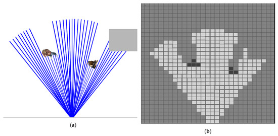
Figure 1.
(a) Shows the top-view of the scene containing people and an object scanned by an RGB-D camera. (b) Shows the obtained occupancy grid of the scene wherein the higher the probability, the darker the cell is, and vice versa.
To update the map, many methods found in the literature used a Bayesian approach [26,27]. They either used the Bayes rule directly or indirectly through one of its derived methods such as Kalman Filter, Particle Filter, etc. The concept behind the Bayes rule is that given some characteristic information and level of confidence about it, it is used to determine the probability a human occupies a given location. Some examples of work which used Bayes rule includes [26,27].
To capture human/victim detection, each cell in the occupancy grid map can hold one of the two distinct states . The probability that a human is observed will be denoted as and probability of non-human is donated as . Practically, determining the probability at specific cell requires the last state on the cell, the observation from the human detection module and the robot motion. Such information is taken into account using the Bayes filter [28].
In this work, three single 2D maps are generated from three different sensors, RGB camera, thermal camera, and wireless sensor. All maps demonstrate the presence of humans and are updated using a Bayesian approach. After that, a merged map is generated by combining the weighted re-scaled maps.
2.3. Exploration
Exploration of unknown environment has been achieved using various methods throughout the literature. Frontier-based [12,13,29] and Next-Best-View (NBV) [14] approaches are the most commonly used approaches. The frontier-based methods aim to explore the frontiers (boundaries between free and unexplored space) of a given area. However, the NBV approaches are used to determine the next viewpoint or candidate position to visit to increase the chance of achieving the objective defined in the utility function. The NBV approach selects the next pose from the list of possible candidates (viewpoints) that score the highest according to the criteria defined in the utility function. The criteria may include: the amount of information that could be potentially obtained by the candidate viewpoint; the execution cost (i.e., energy, path) of the next action [30]; or the distance to be traveled to reach the next best view [14]. Consequently, a proper utility function and information gain prediction have a vital role in NBV selection.
In this research, we use the NBV as it is directly related to the work presented in this paper. The main elements of the NBV approach are viewpoint sampling, viewpoint evaluation, and a termination condition.
2.3.1. Viewpoint Sampling
To determine the next viewpoint to visit in order to maximize the chance of detecting a victim, the common methods sample the space into candidate viewpoints, and evaluate these viewpoints in order to determine which one can provide the best chance of detecting a victim. Different sampling strategies are commonly used in the literature such as (1) Regular Grid Sampling [31], (2) Frontier Sampling [32], and (3) Rapidly exploring Random Trees [33].
In the regular grid sampling, the state space around the robot is discretized based on the number of degrees of freedom (n-DOF) of the robot. Precisely, each degree of the robot is used to divide state space and the possible poses that an n-DOF robot can is visualized as points lying in a discretized n-dimensional space. In the case of 3- dimensional space, the sampled point will look like a crystal lattice; hence the name “state lattice” [31].
In frontier sampling, moving the robot to the boundaries between known and unknown space can maximize the chance of obtaining new information. This approach allows the robot to see beyond the explored map and hence expand the map. Typically, this sampling procedure is done on an occupancy grid map, as it is easy to allocate frontiers where the free and unexplored space presented clearly [13,32].
A simple form of frontier selection is to identify the frontier cell which is closest to the current robot location. Then, the robot moves to that frontier and captures data from its sensor to expand the exploration map. The robot repeats this process until no frontier is left [32,34].
Rapidly exploring Random Trees (RRTs) are another method commonly used to sample in a receding horizon manner [14]. By sampling possible future viewpoints in a geometric random tree, the defined utility function will enable the exploration of unknown volume environment. During this process, a series of random points are generated. Then, these points are connected in a tree-like expanding through explored space. Each branch represents a set of random chains and the branch which maps the unknown space is selected. Each branch of the samples RRT is then evaluated using the defined utility function, and the branch with the best possible exploration outcome is used to select the best new exploration position to travel to.
2.3.2. Viewpoint Evaluation
A utility function is usually used to select the best viewpoint from the list of available candidates generated during the sampling process. Information metric used to evaluate the viewpoints is the information gain [35]. The entropy () for a specific cell x in the occupancy map is given as
From Equation (1), the entropy is a measure of uncertainty associated with the cell probability. is maxed when the all outcomes are equally likely while it is zero when the trial outcomes are certain.
The corresponding view entropy for a specific view denoted by subscript v is the sum on the individual cell’s entropy within the sensor FOV, and defined as:
where N is a normalization factor that represents the number of visible cells in the sampled FOV [36]
An extension of the information gain is the weighted information gain with distance penalty [12], given by:
where is the penalization factor [12].
Another information gain utility function is the max probability. In this method, the viewpoints that contain cells with higher maximum probability are preferred compared to other viewpoints with cells with less maximum probability. This method works well when a victim is found as the next evaluated viewpoints will cover the victim within their FOV aiming to higher or lower the victim detection probability. The evaluation of the max probability gain of a viewpoint [2] is given by:
2.3.3. Termination Conditions
Autonomous exploration tasks terminate once a pre-defined condition has been achieved. There are several type of termination conditions depending on the scenario such as whether a victim was found [37], whether a maximum number of iterations has been reached [38], or whether the information gain reached a max [19,31]. Additionally, for frontier-based methods, the exploration terminates when no more frontiers generated [32].
Our work is different from the state-of-the-art approaches in two elements of the NBV, viewpoint sampling, and viewpoint evaluation. The proposed Adaptive Grid Sampling Approach overcomes the limitation of one of the existing state-of-the-art approaches, which is the Regular Grid Sampling Approach [30,31]. Also, we propose a new viewpoint evaluation (utility function) method to detect a human as fast as possible and reduce the traveled distance. Our viewpoint evaluation function considers occupancy, distance, and victim detection using both the proposed merged map and the proposed sampling approach. The proposed utility function is compared with the state-of-the-art utility functions presented in Equations (3) and (4).
3. Proposed Approach
In this work, a new approach for victim localization, depicted in Figure 2, is presented. The proposed victim localization method consists of two main processes: the victim detection/mapping and the NBV exploration processes. In the first process, victim detection/mapping, the victim is detected and localized in multi-layer maps that are generated by fusing vision, thermal, and wireless data. Victim detection is accomplished by applying a detection algorithm that estimates human location with uncertainty. The victim location is stored in an occupancy grid map, which is recursively updated to increase the confidence in locating the victim. In the second process, exploration, the NBV approach is used, and a new utility function is proposed. The NBV approach includes viewpoint sampling, viewpoint evaluation, navigation, and termination conditions.
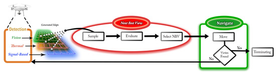
Figure 2.
Flowchart of the System Model.
The novelty of our solution is on the integration of the wireless signal with other various classical sensors to assist in locating victims. This presents a unique solution along with the multi-sensor-based mapping approach and the multi-objective exploration strategy. Furthermore, deep-learning-based human detection is used to detect the presence of a human from a 2D image. This information is then used with a synchronized 3D point cloud to localize the human accurately. Moreover, unlike regular grid sampling approaches, our proposed adaptive viewpoint sampling method solves the local minimum problem. This approach enables rapid exploration and victims’ detection in a USAR environment. Finally, the performance of the proposed approach was compared with other approaches available in the literature, described in Section 4. Results showed that our approach performs better in various metrics such as the number of iterations, traveled distance, and entropy reduction.
3.1. Multi-Sensor Approach for Victim Localization and Mapping
3.1.1. Vision-Based Victim Localization
The procedure for the vision-based victim localization is summarized in Algorithm 1. It involves two main stages: victim detection, where the victim is found in the image frame; and mapping which register the detection confidences in a 2D occupancy grid map.
- Victim Detection: In this work, Single-Shot Multi-box detector (SSD) [21] structure was adapted in our classifier, trained it with visual object class challenge (VOC2007) dataset [39]. The SSD structure is depicted in Figure 3. The input to the detection module is a 2D RGB image and the desired output is a box overlapping the detected human with a probability reflecting the detection confidence. The victim detection aims to find a human in a received RGB image.
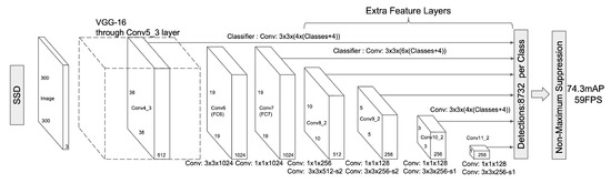 Figure 3. System Model of SSD detector. Taken from [21].
 - Victim Mapping: Based on the analysis of the SSD detector, the minimum size of the detected box in the training-set is pixels. This box size corresponds to in meter. To estimate the distance between the detected human and the camera [40], the ratio of the box to the image is along the y-axis is given as where is re-calculated for the tangent of the half-angle under which you see the object which given as . The distance d to the camera is estimated as . The victim will appropriately be located if its distance separation from the camera is within the camera depth operational range.
| Algorithm 1 Vision-Based Victim Localization Scheme |
Input:
2: ▹ where is a matrix containing Box coordinates, represents the box coordinates, and is a vector containing the human corresponding probabilities 3 for i=1:length() do 4: if then 5: 6: 7: if is empty then 8: 9: end if 10: sort in ascending order 11: 12: 13: project P in x-y plane 14: ▹ append to the list of victim locations 15: end if 16: end for 17: for all cells do 18: for all do 19: 20: 21: 22: end for 23: 24: 25: end for |
3.1.2. Thermal-Based Victim Localization
The procedure for thermal-based victim localization summarized in Algorithm 2 involves two stages: victim detection, where the victim is found in the thermal image based on heat signature; and thermal occupancy mapping; where detection confidences obtained from the thermal detector is stored.
- Victim Detection: Thermal detection is used to detect human heat signature presented using the infrared light which is part of the electromagnetic (EM) spectrum. This approach is useful when the human cannot be detected in RGB images, especially, in dark lighting condition. The method adopted here is a simple blob detector which locates blobs in a thermal image for a temperature range of to (normal human temperature). The procedures for thermal detection is presented in Figure 4 which is composed of three stages. In the first stage, the thermal images are converted into mono-image. Then, two thresholds, and are applied to the mono-image to get a binary image that correspond . After that, contouring is done to extract regions which represented the human thermal location. The blob detector was implemented using OpenCV where the minimum blob area is set to 20 pixels and a minimum adjacent distance between blob is set to 25 pixels. A human face was detected as shown in Figure 4. A full-human body can also be detected using the thermal detector by relaxing the choice of and .
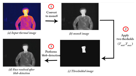 Figure 4. Demonstration of thermal detection using the Optris PI200.
 - Victim Mapping: After a box is resolved on the human thermal image, the center of the box is calculated in the image frame give asThen a ray is broadcast from the thermal camera center through the obtained pixel. After identifying the corresponding 3D ray in the world frame, orthogonal projection is deployed as where the is removed. The final location is stored as .
The thermal map is updated when using 2D rays by assigning to 0.6 for the cells corresponding to the 2-D ray and 0.4 for the other cells within the camera FOV. Then is obtained by finding the belief distribution at time t using the previous where and . Both control and the distribution of the state are used to determine the distribution of the current state . This step is known as the prediction. When the state space is finite, the integral in results in a finite sum. The used here for normalization, to make sure that the resulting product is a probability function whose integral is equal to 1. The map resolution is set to 0.2 m as the thermal-based victim localization is a bearing-only localization and required multiple ray generations of different poses to sufficiently locate a victim as shown in Figure 5.
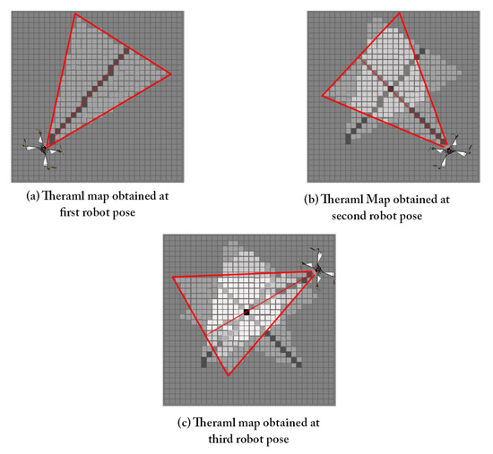
Figure 5.
Thermal map update for three different robot poses.
| Algorithm 2 Thermal-Based Victim Localization Scheme |
Input:
2: 3: for all pixels p∈ do 4: if then 5: 6: else 7: 8: end if 9: end for 10: ▹ where is a matrix containing detected Box coordinates in represents the box coordinates 11: if is not empty then 12: 13: for all boxes c in do 14: generate 2-D line, , that pass through the center of box c and terminate at the end of 15: ▹ append to the list of rays 16: end for 17: end if 18: for all cells do 19: for all do 20: 21: 22: 23: end for 24: 25: 26: end for |
3.1.3. Wireless-Based Victim Localization
In the literature, many various techniques are used to find the distance or the angle to localize an unknown static node which in this work is assumed to be the cell-phone of the victim. One of the popular methods for the ranging techniques is the Received Signal Strength (RSS) which provides a distance indication to the unknown node. The robot will act as a moving anchor node and captures multiples RSS readings with the aim of locating the victim. The proposed system assumes the transmission power of victim wireless device is fixed and known. This section explains the log-normal channel model which adopted in the wireless detection module. Also, the updating procedure for the captured measurement is explained to speed up the victim search.
- Victim Detection: A victim can be detected wirelessly by monitoring a given transmitted signal from the victim phone. In this configuration, the victim phone can be treated as a transmitter while the wireless receiver can be placed on a robot. If no obstacle between the transmitter and receiver is found, the free-space propagation model is used to predict the Received Signal Strength in the line-of-sight (LOS) [41]. The RSS equation is derived from Friis Transmission formula [42]where is the Received Signal Strength from receiver node i at node transmitter node j at time t, is the transmitted power, is the transmitter gain, is the receiver gain, is the distance from sensor node i at node j, and is the wavelength of the signal. From Equation (6), the received power attenuates exponentially with the distance [41]. The free-space path loss is derived from the equation above by 10 log the ratio of the transmitted power to the received power and setting = = 1 because, in most of the cases, the used antennas are isotropic antennas, which radiate equally in all direction, giving constant radiation pattern [41]. Thus, the formula is the following:When using the free-space model, the average received signal decreases with the distance between the transmitter and receiver in all the other real environments in a logarithmic way. Therefore, the path-loss model generalized form can be obtained by changing the free-space path loss with the path-loss exponent n depending on the environment, which is known as the log-distance path-loss model which will result in the following formula [41]:where is the reference distance at which the path loss inherits the characteristics of free space in (7) [41]. Every path between the transmitter and the receiver has different path loss since the environment characteristics changes as the location of the receiver changes. Moreover, the signal may not penetrate in the same way. For that reason, more realistic modeling of the transmission is assumed which is the log-normal modeling.where = − is the path loss at distance from the transmitter, is the path-loss model at the reference distance which is constant. is Gaussian random variable with a zero mean and standard deviation [43].Due to the presence of noise in the log-normal model, the path loss will be different even the same location with distance . To obtain a relatively stable reading, is recording for K samples, then, an averaging process is done to get the measured . The victim can be set to be identified wireless if the detected distance is less than a specific distance threshold . This is because RSS reading is high when the transmitter is closer to the receiver leading to a less noise variance. Hence, from a log-normal model, it is sufficient to state that the victim is found in the measured distance satisfy the conditionThe same idea is used in weighted least-square approach where high weights are given for low distances leading to a less RMSE in the localized node when compared to the conventional lease-square approach which assumes constant noise variance across all measured distances [44].
- Victim Mapping: When RSS is used to locate an unknown node, a single measured distance is not sufficient because the unknown node can be anywhere over a circle with radius equal to the distance. That can be solved using trilateration as shown in Figure 6. In 2D space, trilateration requires at least three-distance measurements from anchor nodes. The location of the unknown node is the intersection of the three circles as show in Figure 6 [45].
 Figure 6. TrilaterationUsing trilateration can lead to a problem in case all the measured distances are large (with high noise variance), which can lead to a false located position. To alleviate this problem, the use of occupancy grid is proposed when updating the map. The measured distance is compared based on the criteria . If this criteria it met, the measurement is trusted, and the map is updated with victim probability within a circle of radius equal to . Otherwise, the measured distance is discarded. The updating process is shown in Figure 7.
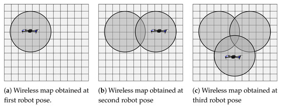 Figure 7. Wireless map update for three different robot poses.
3.1.4. Multi-Sensor Occupancy Grid Map Merging
In this work, three different victim-location maps are generated using three different sensors. The probability of the victim’s presence in each map is obtained by the Bayesian-probabilistic framework independently. These maps are then fused in a Bayesian-probabilistic framework to obtain a merged map that indicates human presence probability. Following the Bayesian approach in generating the multi-sensor occupancy grid may introduce undesired errors. For example, some victim detectors may have less confidence compared to others due to sensor limitations. For this reason, multiple sensors with different weights can be used for each victim detector. Let D represents a victim detector and is the confidence assigned for each detector. Each of the victim detectors gives two quantities, which are the measured probability of finding a human given detector D and the weight that reflects how much confidence assigned to a victim detector. The posterior probability is given as:
where is a normalized factor for all the weights. Figure 8 shows the process of updating a single cell in the combined map taken into consideration the different weights for the victim modules implemented in each map. Let be the combined map from the three sensors. The merged map from the three sensors is used to monitor the maximum probability. The merged map is obtained by re-scaling the three occupancy maps to the smallest resolution which is the lowest resolutions of the three used maps. The combined map is given as
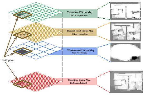
Figure 8.
Merged map obtained from three maps of different resolutions where a single cell update is highlighted.
3.2. Exploration
We adapt the NBV approach to explore the environment. The typical pipeline for NBV includes viewpoint sampling, viewpoint evaluation, navigation and termination. In this work, two viewpoint sampling methods are used for NBV evaluation and viewpoint selection which are the Regular Grid Sampling Approach (RGSA) and a proposed Adaptive Grid Sampling Approach (AGSA). After that, the different sample viewpoint are evaluated using a utility function. Then, the robot navigates to the selected viewpoint and update the maps simultaneously. The search mission is terminated when a termination condition is met.
In this work, the search process terminates when a victim is found or when all the viewpoints provide a zero reward from the utility. The victim is assumed to be found in the maximum probability if the occupancy map went above a specific threshold or if the number of iteration exceeded a pre-defined number of iterations.
The proposed NBV approach uses a multi-objective utility function which is composed of three components. The first function is the information gain, which focuses on the exploration objective while the function is biased towards exploring occupancy grids with higher victim presence probability. Traveling further distances is penalized by the function to compromise between satisfying the objectives and the traveling cost. The multi-objective utility defined as:
where , P is the probability of a cell in a viewpoint, is the maximum probability cell within a given viewpoint, is the information gain (IG) for a given viewpoint, d is the distance from the current location to the evaluated viewpoint, is the exponential penalization parameter while , and are the weights used to control each of the three objectives. The impact of on the selectivity of is illustrated in Figure 9, used to control how much emphasis should be put on victim detection vs environment exploration.
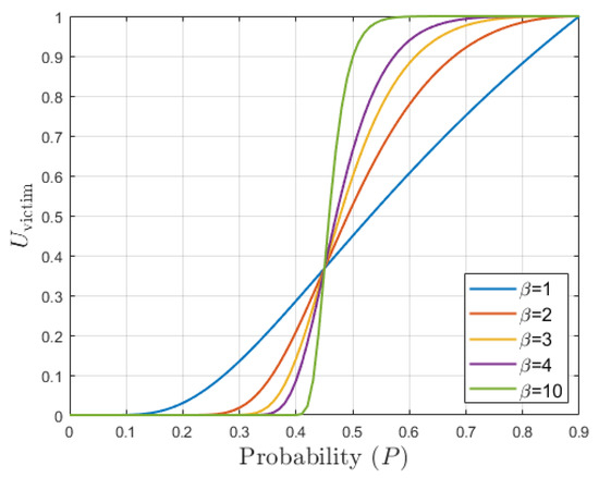
Figure 9.
Impact of the parameter on the selectivity of function where .
After viewpoint evaluation, different navigation schemes are used based on the selected view generation method. For Regular Grid Sampling approach, a collision-checking is performed over the line between the vehicle and the evaluated viewpoint, to ensure that the path is safe for the drone to traverse. For adaptive sampling, initially, a straight line is performed. In case it failed, then an A* [46] planner is used.
Upon finding a victim, the search process is terminated to allow the robot to report back the victim location to the rescue team. The victim is assumed to be found in the maximum probability if the occupancy map went above a specific threshold or if the number of iteration exceeded a pre-defined number of iterations. This method can also be extended to incorporate more than one victim.
4. Experimental Results
Simulation experiments were performed on an Asus-ROG-STRIX Laptop (Intel Core i7-6700HQ @ 2.60 GHz × 8, 15.6 GB RAM). The victim localization system was implemented on Ubuntu-kinetic 16.04 using the Robot Operating System (ROS) [47], where the system consists of a group of nodes with data sharing capability. Hence, the use of ROS simply the direct implementation of the system on the hardware platform. The environment was simulated using Gazebo, and the code programmed in both C++ and Python. The GridMap library [48] was used to represent the 2-D occupancy grid, navigation was done using Octomap [49] and point cloud data (PCL) was handled using the Point Cloud Library (PCL) [50]. An open source implementation of the proposed approach can be found at [51] for further use.
4.1. Vehicle Model and Environment
The adopted vehicle model in the tests is based on a floating sensor approach, where the sensor moves virtually in space and captures data from the selected viewpoints. The floating sensor is presented as a virtual common base link among candidate sensors. Static transformations are used to refer the sensors links to the floating sensor base link. Upon moving the floating sensor, the way-point command is applied in the floating sensor local frame where the sensors take their new positions based on their respective transformations. Figure 10 shows the floating sensor along with its components. By using the floating sensor approach we skip continuous data that could be acquired during the transition between the viewpoints, resulting in a better evaluating setup where only data and information gathered from the viewpoints is used to conduct the exploration and victim detection. The system is equipped with three sensors, namely an RGB-D camera, a thermal camera, and a wireless adapter. The specifications of the RGB-D camera, thermal camera, and wirelesses transmitter specifications are presented in Table 1. Both RGB-D and thermal camera are mounted underneath to increase the unobstructed field of view (FOV). The proposed system can adapt to any UAVs.
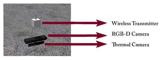
Figure 10.
Floating sensor model.

Table 1.
RGB camera, Thermal camera, and Wireless Sensor specifications.
The simulated environment is shown in Figure 11 with dimensions 13 m × 15 m. This environment has multiple rooms with dead-ends and a corridor which can demonstrate the problems that the system can experiences and how to be tackled. Due to the difficulty in simulating an actual heat signature in the environment, the output of the thermal blob detector is simulated by the detection of the victim red-shirt from the captured RGB image.
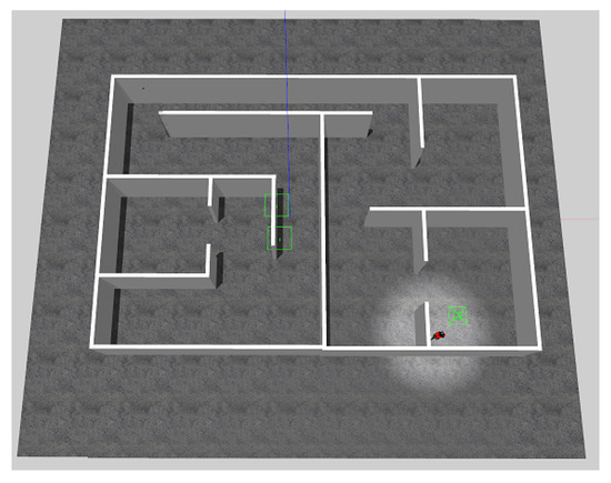
Figure 11.
Simulated environment.
4.2. Tests Scenario and Parameters
The tests are carried out to show the effectiveness of the proposed approach, namely the combined map, viewpoint sampling method, and the multi-objective utility function. The executed tests are divided into two classes based on the sampling approaches, Regular Grid Sampling Approach (RGSA) and the proposed Adaptive Grid Sampling Approach (AGSA). The proposed AGSA is compared with the state-of-the-art RGSA [30,31]. In each sampling approach, the proposed merged map including the wireless map, is compared with the state-of-the-art single generated maps using single sensor. In addition, the proposed utility () function is compared with the state-of-the-art utility functions () and (), weighted information gain [12] obtained using Equation (3) and max probability [2] obtained using Equation (4), respectively. The evaluation metrics used for each test are the number of iteration, distance traveled, and entropy reduction. The parameters used for RGSA and AGSA are shown in Table 2 and Table 3, respectively.
Table 2.
Regular Grid Sampling Approach Parameters.
Table 3.
Adaptive Grid Sampling Approach Parameters.
In each test, the four different maps: vision, thermal, wireless, and merged map were used to test their performance. The viewpoint evaluation is executed using the three utilities: weighted information gain (), improved max utility (), and the proposed multi-objective utility (). Table 4 lists the parameters used in the map generation.
Table 4.
Parameters used in the simulation.
The Octomap resolution is set to 0.2 m. A termination condition of maximum iteration is used in all the tests where the maximum iteration is set to 120, and the victim probability threshold is set to 0.9 (the probability at which a victim is considered found). For the utilities, The distance weight is set to 0.05, while for the proposed utilities, the weights are selected as and when evaluated in the vision and thermal map. For the wireless map, it is assigned as and . The penalization parameter is set to 1. The metrics used in the evaluation are the total number of iterations before termination (It), total map entropy before the victim search begin subtracted by total map entropy after the victim is found (TER), and the total distance traveled in meters (D). Some of the parameters used during the experimentation were carefully tuned to achieve the optimum setup given the experimental environment. The benchmarking, however, was conducted with the same parameters for all the methods.
4.3. Regular Grid Sampling Approach (RGSA) Results
The obtained results of the different utility functions are shown in Figure 12a in terms of entropy and Figure 12b in terms of distance traveled. For comparison, the same results listed in Table 5.
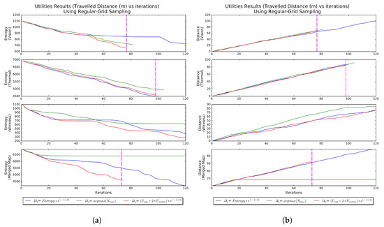
Figure 12.
Regular Grid Sampling Approach Results. (a) Entropy vs. Iteration using Regular Grid Sampling Approach. The fastest method is indicated by the magenta vertical dash line. (b) Distance vs. Iteration using Regular Grid Sampling Approach. The fastest method is indicated by the magenta vertical dash line.
Table 5.
Results of RGSA tests. VF: victim Found It: Iterations, D: Distance, TER: Total Entropy Reduction. The numbers in bold indicate better performance.
In the vision map, the proposed utility () has fewer iterations (77), entropy reduction, and distance traveled when compared to the other utilities within the same map. It is also noticeable that the weighed information gain () failed to find the victim as it exceeds the maximum iteration 120. This because of experience a local minimum indicated by the stabilized entropy curve for an extended number of iterations. The max utility () succeeded in locating the victim but with a relatively higher number of iterations as this utility does not have an exploration capability.
In the thermal map, has fewer iterations (98), and distance traveled when compared to the other utilities within the same map. Also, has more iterations but a better entropy reduction compared to . has the worst performance with a higher number of iterations and distance travel to locate the victim.
In the wireless map, all the three methods failed in locating the victim where the total iterations reached the maximum allowable iteration. That is due to the nature of the wireless transmitter wherein the map update is done in a circular manner making it easy for the robot to fall in a local minimum.
In the merged map, has the best performance with a lower number of iterations (73), entropy reduction and distance traveled compared to the other utilities in the same map as well as across all maps. In , the method failed to locate the victim as the vehicle experience a set of local minima which was mainly inherited from the wireless component. The merged map with failed because the utility falls in an inescapable local minimum. Figure 13 shows the path trajectory of the vehicle in -merged test using RGSA.
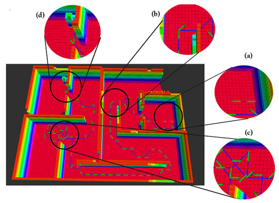
Figure 13.
Vehicle traversed path in the -merged test using RGSA where (a) start location, (b) direct-path trajectory, (c) location of the detected local minimum where A* Planner was invoked to generate path, (d) end location.
4.4. Adaptive Grid Sampling Approach (AGSA) Results
Here, the Adaptive Grid Sampling Approach (AGSA) is used to test the performance of the utilities when implemented on the individual maps as well as the merged map. The settings used in the AGSA are shown in Table 3. The obtained results of the different tests shown in Figure 14a in terms of entropy and Figure 14b in terms of distance traveled. Also, the instants when the AGSA detected local minimum as shown in Figure 15. For comparison, the same results listed in Table 6.
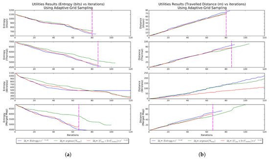
Figure 14.
Regular Adaptive Grid Sampling Approach Results. (a) Entropy vs. Iteration using Adaptive Grid Sampling Approach. The fastest method is indicated by the magenta vertical dash line. (b) Travel distance vs. Iteration using Adaptive Grid Sampling Approach. The fastest method is indicated by the magenta vertical dash line.
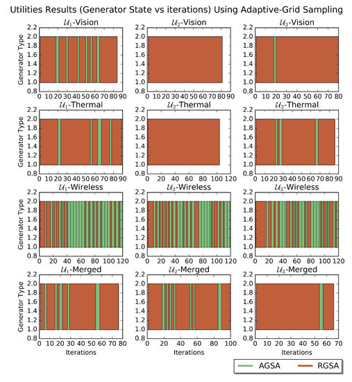
Figure 15.
Generator states vs. iterations using Adaptive Grid Sampling Approach.
Table 6.
Results of AGSA tests. VF: victim Found It: Iterations, D: Distance, TER: Total Entropy Reduction. The numbers in bold indicate better performance.
In the vision map, the proposed utility () has fewer iterations to find the victim (80). The weighed information gain () succeeds due to the local minimum’s problem been mitigated by the AGSA. The max utility () has the same performance as in the case of RGSA. That is because the works by selecting a viewpoint with maximum entropy, making it hard to fall under the threshold .
In the thermal map, has fewer iterations to find the victim (86). In comparison to , has a lower entropy reduction but more iterations to locate the victim. has the worst performance compared to the rest of the method. Also, the performance is the same as in the case of RGSA. In the wireless map, all the utilities failed, as they require more iterations to find the victim.
In the merged map, has fewer iterations to find the victim (66). Unlike in RGSA, succeeds in locating the victim as the vehicle was able to escape local minima. failed in locating the victim as this method does not encourage the vehicle to explore upon initial detection of the victim. That can lead to a problem if the victim is located through the wireless sensor, but an obstacle such as a wall occludes the victim. Under this scenario, it is preferable to explore and found a line-of-sight with the victim allowing the vision and the thermal module to operate, a feature the max utility is lacking.
Across all the tests, -merged using ARGS has the best performance in terms of iterations and distance travel with a relatively better entropy reduction.
Figure 16 shows the traveled path of the vehicle in the -merged test using AGSA. A video that demonstrates the efficiency of indoor environment exploration using AGSA is provided in [52]. A video that represents a real-time experiment for victim detection is shown in [53], which was conducted to demonstrate the effectiveness of the proposed work.
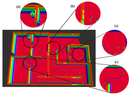
Figure 16.
Vehicle traversed path in the -merged test using AGSA where (a) start location, (b) direct-path trajectory, (c) location of the detected local minimum where A* Planner was invoked to generate path, (d) end location.
4.5. Discussion Results
The best performance was obtained when merging the probabilistic information in an occupancy grid map, and using it to guide the search strategy. In this case, the combined information merged in a probabilistic Bayesian framework is used instead of local optima of each system individually.
Using the Adaptive Grid Sampling Approach (AGSA), the proposed merged map with the proposed utility function outperforms both traditional single-vision and thermal maps using the proposed utility function on the number of iteration and the traveled distance. The reduction in the number of iteration was in a range of 17.5% to 23.25% while the reduction in the traveled distance was in a range of 10% to 18.5% respectively.
In addition, using the Regular Grid Sampling Approach (RGSA), the proposed merged map with the proposed utility function outperforms both proposed single-vision map and single-thermal map using proposed utility function on the number of iteration and the traveled distance. The reduction in the number of iteration was in a range of 5.2% to 25.5% while the reduction in the traveled distance was in a range of 5.4% to 23%, respectively.
Hence, the merged map results in a moderate performance over the other single maps when using the Regular Grid Sampling Approach. However, combining the merged map with the Adaptive Grid Sampling Approach presents higher performance.
5. Conclusions
In this work we proposed an USAR exploration approach based on multi-sensor fusion that uses vision, thermal, and wireless sensors to generate a probabilistic 2D victim-location maps. A multi-objective utility function exploited the fused 2D victim-location map to generate and evaluate viewpoints in a NBV fashion. The evaluation process targets three desired objectives, specifically exploration, victim detection, and traveled distance. Additionally, an adaptive grid sampling algorithm (AGSA) was proposed to resolve the local minimum issue occurs in the Regular Grid Sampling Approach (RGSA). Experimental results showed that the merged map results in a moderate performance over the other single maps when using the Regular Grid Sampling Approach. However, combining the merged map with the Adaptive Grid Sampling Approach presents higher performance. In both cases, the results demonstrated that the proposed utility function using merged map performs better than methods that rely on a single sensor in the time it takes to detect the victim, distance traveled, and information gain reduction. The tests were conducted in a monitored environment yet there are different sources of uncertainty. In future work, we will extend the system to address these uncertainty with scalability, and conduct experimental tests in real-world scenarios.
Author Contributions
Conceptualization, A.G., R.A., T.T., and N.A.; methodology, A.G., R.A. and T.T.; software, A.G., R.A., and T.T.; validation, A.G. and T.T. formal analysis, A.G., R.A., U.A., and T.T.; investigation, A.G., R.A., U.A., and T.T.; resources, A.G., U.A., T.T., N.A., and R.A.; data curation, A.G., R.A., and T.T.; writing—original draft preparation, A.G. and R.A.; writing—review and editing, R.A. and T.T.; visualization, A.G., R.A.; supervision, T.T., N.A., and L.S.; project administration, T.T., N.A., and L.S.
Funding
This work was supported by ICT fund for “A Semi Autonomous Mobile Robotic C4ISR System for Urban Search and Rescue” project.
Acknowledgments
This publication acknowledges the support by the Khalifa University of Science and Technology under Award No. RC1-2018-KUCARS.
Conflicts of Interest
The authors declare no conflict of interest.
References
- Naidoo, Y.; Stopforth, R.; Bright, G. Development of an UAV for search & rescue applications. In Proceedings of the IEEE Africon’11, Livingstone, Zambia, 13–15 September 2011; pp. 1–6. [Google Scholar]
- Waharte, S.; Trigoni, N. Supporting Search and Rescue Operations with UAVs. In Proceedings of the 2010 International Conference on Emerging Security Technologies, Canterbury, UK, 6–7 September 2010; pp. 142–147. [Google Scholar] [CrossRef]
- Erdelj, M.; Natalizio, E.; Chowdhury, K.R.; Akyildiz, I.F. Help from the sky: Leveraging UAVs for disaster management. IEEE Pervasive Comput. 2017, 16, 24–32. [Google Scholar] [CrossRef]
- Kohlbrecher, S.; Meyer, J.; Graber, T.; Petersen, K.; Klingauf, U.; von Stryk, O. Hector Open Source Modules for Autonomous Mapping and Navigation with Rescue Robots. In RoboCup 2013: Robot World Cup XVII; Behnke, S., Veloso, M., Visser, A., Xiong, R., Eds.; Springer: Berlin/Heidelberg, Germany, 2014; pp. 624–631. [Google Scholar]
- Milas, A.S.; Cracknell, A.P.; Warner, T.A. Drones—The third generation source of remote sensing data. Int. J. Remote Sens. 2018, 39, 7125–7137. [Google Scholar] [CrossRef]
- Malihi, S.; Valadan Zoej, M.; Hahn, M. Large-Scale Accurate Reconstruction of Buildings Employing Point Clouds Generated from UAV Imagery. Remote Sens. 2018, 10, 1148. [Google Scholar] [CrossRef]
- Balsa-Barreiro, J.; Fritsch, D. Generation of visually aesthetic and detailed 3D models of historical cities by using laser scanning and digital photogrammetry. Digit. Appl. Archaeol. Cult. Herit. 2018, 8, 57–64. [Google Scholar] [CrossRef]
- Wang, Y.; Tian, F.; Huang, Y.; Wang, J.; Wei, C. Monitoring coal fires in Datong coalfield using multi-source remote sensing data. Trans. Nonferrous Met. Soc. China 2015, 25, 3421–3428. [Google Scholar] [CrossRef]
- Kinect Sensor for Xbox 360 Components. Available online: https://support.xbox.com/ar-AE/xbox-360/accessories/kinect-sensor-components (accessed on 13 November 2019).
- FLIR DUO PRO R 640 13 mm Dual Sensor. Available online: https://www.oemcameras.com/flir-duo-pro-r-640-13mm.htm (accessed on 13 November 2019).
- Hahn, R.; Lang, D.; Selich, M.; Paulus, D. Heat mapping for improved victim detection. In Proceedings of the 2011 IEEE International Symposium on Safety, Security, and Rescue Robotics, Kyoto, Japan, 1–5 November 2011; pp. 116–121. [Google Scholar]
- González-Banos, H.H.; Latombe, J.C. Navigation strategies for exploring indoor environments. Int. J. Robot. Res. 2002, 21, 829–848. [Google Scholar] [CrossRef]
- Cieslewski, T.; Kaufmann, E.; Scaramuzza, D. Rapid Exploration with Multi-Rotors: A Frontier Selection Method for High Speed Flight. In Proceedings of the 2017 IEEE/RSJ International Conference on Intelligent Robots and Systems (IROS 2017), Vancouver, BC, Canada, 24–28 September 2017. [Google Scholar]
- Bircher, A.; Kamel, M.; Alexis, K.; Oleynikova, H.; Siegwart, R. Receding Horizon “Next-Best-View” Planner for 3D Exploration. In Proceedings of the 2016 IEEE International Conference on Robotics and Automation (ICRA), Stockholm, Sweden, 16–21 May 2016; pp. 1462–1468. [Google Scholar] [CrossRef]
- Portmann, J.; Lynen, S.; Chli, M.; Siegwart, R. People detection and tracking from aerial thermal views. In Proceedings of the 2014 IEEE International Conference on Robotics and Automation (ICRA), Hong Kong, China, 31 May–7 June 2014; pp. 1794–1800. [Google Scholar] [CrossRef]
- Riaz, I.; Piao, J.; Shin, H. Human detection by using centrist features for thermal images. In Proceedings of the IADIS International Conference Computer Graphics, Visualization, Computer Vision and Image Processing, Prague, Czech Republic, 22–24 July 2013. [Google Scholar]
- Uzun, Y.; Balcılar, M.; Mahmoodi, K.; Davletov, F.; Amasyalı, M.F.; Yavuz, S. Usage of HoG (histograms of oriented gradients) features for victim detection at disaster areas. In Proceedings of the 2013 8th International Conference on Electrical and Electronics Engineering (ELECO), Bursa, Turkey, 28–30 November 2013; pp. 535–538. [Google Scholar]
- Sulistijono, I.A.; Risnumawan, A. From concrete to abstract: Multilayer neural networks for disaster victims detection. In Proceedings of the 2016 International Electronics Symposium (IES), Denpasar, Indonesia, 29–30 September 2016; pp. 93–98. [Google Scholar]
- Abduldayem, A.; Gan, D.; Seneviratne, L.D.; Taha, T. 3D Reconstruction of Complex Structures with Online Profiling and Adaptive Viewpoint Sampling. In Proceedings of the International Micro Air Vehicle Conference and Flight Competition, Toulouse, France, 18–21 September 2017; pp. 278–285. [Google Scholar]
- Xia, D.X.; Li, S.Z. Rotation angle recovery for rotation invariant detector in lying pose human body detection. J. Eng. 2015, 2015, 160–163. [Google Scholar] [CrossRef]
- Liu, W.; Anguelov, D.; Erhan, D.; Szegedy, C.; Reed, S.; Fu, C.Y.; Berg, A.C. SSD: Single shot multibox detector. In Lecture Notes in Computer Science; Springer International Publishing: New York, NY, USA, 2016; pp. 21–37. [Google Scholar] [CrossRef]
- Zhang, L.; Lin, L.; Liang, X.; He, K. Is Faster R-CNN Doing Well for Pedestrian Detection? arXiv 2016, arXiv:1607.07032. [Google Scholar]
- Louie, W.Y.G.; Nejat, G. A victim identification methodology for rescue robots operating in cluttered USAR environments. Adv. Robot. 2013, 27, 373–384. [Google Scholar] [CrossRef]
- Hadi, H.S.; Rosbi, M.; Sheikh, U.U.; Amin, S.H.M. Fusion of thermal and depth images for occlusion handling for human detection from mobile robot. In Proceedings of the 2015 10th Asian Control Conference (ASCC), Kota Kinabalu, Malaysia, 31 May–3 June 2015; pp. 1–5. [Google Scholar] [CrossRef]
- Hu, Z.; Ai, H.; Ren, H.; Zhang, Y. Fast human detection in RGB-D images based on color-depth joint feature learning. In Proceedings of the 2016 IEEE International Conference on Image Processing (ICIP), Phoenix, AZ, USA, 25–28 September 2016; pp. 266–270. [Google Scholar] [CrossRef]
- Utasi, Á.; Benedek, C. A Bayesian approach on people localization in multicamera systems. IEEE Trans. Circuits Syst. Video Technol. 2012, 23, 105–115. [Google Scholar] [CrossRef]
- Cho, H.; Seo, Y.W.; Kumar, B.V.K.V.; Rajkumar, R.R. A multi-sensor fusion system for moving object detection and tracking in urban driving environments. In Proceedings of the 2014 IEEE International Conference on Robotics and Automation (ICRA), Hong Kong, China, 31 May–7 June 2014; pp. 1836–1843. [Google Scholar] [CrossRef]
- Bongard, J. Probabilistic Robotics. Sebastian Thrun, Wolfram Burgard, and Dieter Fox. (2005, MIT Press.) 647 pages. Artif. Life 2008, 14, 227–229. [Google Scholar] [CrossRef]
- Yamauchi, B. A frontier-based approach for autonomous exploration. In Proceedings of the 1997 IEEE International Symposium on Computational Intelligence in Robotics and Automation (CIRA’97), Monterey, CA, USA, 10–11 July 1997; pp. 146–151. [Google Scholar]
- Heng, L.; Gotovos, A.; Krause, A.; Pollefeys, M. Efficient visual exploration and coverage with a micro aerial vehicle in unknown environments. In Proceedings of the 2015 IEEE International Conference on Robotics and Automation (ICRA), Seattle, WA, USA, 26–30 May 2015; pp. 1071–1078. [Google Scholar]
- Paul, G.; Webb, S.; Liu, D.; Dissanayake, G. Autonomous robot manipulator-based exploration and mapping system for bridge maintenance. Robot. Auton. Syst. 2011, 59, 543–554. [Google Scholar] [CrossRef]
- Al khawaldah, M.; Nuchter, A. Enhanced frontier-based exploration for indoor environment with multiple robots. Adv. Robot. 2015, 29. [Google Scholar] [CrossRef]
- Karaman, S.; Frazzoli, E. Sampling-based algorithms for optimal motion planning. Int. J. Robot. Res. 2011, 30, 846–894. [Google Scholar] [CrossRef]
- Verbiest, K.; Berrabah, S.A.; Colon, E. Autonomous Frontier Based Exploration for Mobile Robots. In Intelligent Robotics and Applications; Lecture Notes in Computer Science; Springer: Cham, Switzerland, 2015; pp. 3–13. [Google Scholar] [CrossRef]
- Delmerico, J.; Isler, S.; Sabzevari, R.; Scaramuzza, D. A comparison of volumetric information gain metrics for active 3D object reconstruction. Auton. Robots 2018, 42, 197–208. [Google Scholar] [CrossRef]
- Kaufman, E.; Lee, T.; Ai, Z. Autonomous exploration by expected information gain from probabilistic occupancy grid mapping. In Proceedings of the 2016 IEEE International Conference on Simulation, Modeling, and Programming for Autonomous Robots (SIMPAR), San Francisco, CA, USA, 13–16 December 2016; pp. 246–251. [Google Scholar] [CrossRef]
- Batista, N.C.; Pereira, G.A.S. A Probabilistic Approach for Fusing People Detectors. J. Control Autom. Electr. Syst. 2015, 26, 616–629. [Google Scholar] [CrossRef]
- Isler, S.; Sabzevari, R.; Delmerico, J.; Scaramuzza, D. An Information Gain Formulation for Active Volumetric 3D Reconstruction. In Proceedings of the 2016 IEEE International Conference on Robotics and Automation (ICRA), Stockholm, Sweden, 16–21 May 2016; pp. 3477–3484. [Google Scholar]
- Everingham, M.; Van Gool, L.; Williams, C.K.I.; Winn, J.; Zisserman, A. The PASCAL Visual Object Classes Challenge 2007 (VOC2007) Results. Available online: http://host.robots.ox.ac.uk/pascal/VOC/voc2007/workshop/index.html (accessed on 13 November 2019).
- Hartley, R.; Zisserman, A. Multiple View Geometry in Computer Vision, 2nd ed.; Cambridge University Press: Cambridge, UK; New York, NY, USA, 2004. [Google Scholar]
- Pozar, D.M. Microwave and Rf Design of Wireless Systems, 1st ed.; Wiley: Hoboken, NJ, USA, 2000. [Google Scholar]
- Kulaib, A.R. Efficient and Accurate Techniques for Cooperative Localization in Wireless Sensor Networks. Ph.D. Thesis, Khalifa University, Abu Dhabi, UAE, 2014. [Google Scholar]
- Tran-Xuan, C.; Vu, V.H.; Koo, I. Calibration mechanism for RSS based localization method in wireless sensor networks. In Proceedings of the 11th International Conference on Advanced Communication Technology (ICACT 2009), Phoenix Park, Korea, 15–18 February 2009; Volume 1, pp. 560–563. [Google Scholar]
- Tarrío, P.; Bernardos, A.M.; Casar, J.R. Weighted least squares techniques for improved received signal strength based localization. Sensors 2011, 11, 8569–8592. [Google Scholar] [CrossRef]
- Patwari, N.; Ash, J.; Kyperountas, S.; Hero, A.; Moses, R.; Correal, N. Locating the nodes: cooperative localization in wireless sensor networks. IEEE Signal Proc. Mag. 2005, 22, 54–69. [Google Scholar] [CrossRef]
- Zeng, W.; Church, R.L. Finding shortest paths on real road networks: The case for A. Int. J. Geogr. Inf. Sci. 2009, 23, 531–543. [Google Scholar] [CrossRef]
- Koubâa, A. Robot Operating System (ROS): The Complete Reference (Volume 1), 1st ed.; Springer International Publishing: Heidelberg, Germany, 2016. [Google Scholar]
- Fankhauser, P.; Hutter, M. A universal grid map library: Implementation and use case for rough terrain navigation. In Robot Operating System (ROS); Koubaa, A., Ed.; Studies in Computational Intelligence; Springer: Cham, Switzerland, 2016; pp. 99–120. [Google Scholar]
- Hornung, A.; Wurm, K.M.; Bennewitz, M.; Stachniss, C.; Burgard, W. OctoMap: An efficient probabilistic 3D mapping framework based on octrees. Auton. Robots 2013, 34, 189–206. [Google Scholar] [CrossRef]
- Rusu, R.B.; Cousins, S. 3D is here: Point Cloud Library (PCL). In Proceedings of the IEEE International Conference on Robotics and Automation (ICRA), Shanghai, China, 9–13 May 2011. [Google Scholar]
- Goian, A. Open Source Implementation of the Proposed Algorithm as a ROS Package. Available online: https://github.com/kucars/victim_localization (accessed on 13 November 2019).
- Ashour, R. Indoor Environment Exploration Using Adaptive Grid Sampling Approach, 2019. Available online: https://youtu.be/4-kwdYb4L-g (accessed on 13 November 2019).
- Ashour, R. Victim Localization in USAR Scenario Exploiting Multi-Layer Mapping Structure, 2019. Available online: https://youtu.be/91vIhmp8vYI (accessed on 13 November 2019).
© 2019 by the authors. Licensee MDPI, Basel, Switzerland. This article is an open access article distributed under the terms and conditions of the Creative Commons Attribution (CC BY) license (http://creativecommons.org/licenses/by/4.0/).