Letter

Analysis of the Optimal Wavelength for Oceanographic Lidar at the Global Scale Based on the Inherent Optical Properties of Water

1
Department of Marine Technology, Ocean University of China, Qingdao 266100, China
2
National Laboratory for Marine Science and Technology, Qingdao 266100, China
*
Author to whom correspondence should be addressed.
Remote Sens. 2019, 11(22), 2705; https://doi.org/10.3390/rs11222705
Submission received: 19 October 2019 / Revised: 13 November 2019 / Accepted: 16 November 2019 / Published: 19 November 2019

Abstract

:
Understanding the optimal wavelength for detecting the water column profile from a light detection and ranging (lidar) system is important in the design of oceanographic lidar systems. In this research, the optimal wavelength for detecting the water column profile using a lidar system at the global scale was analyzed based on the inherent optical properties of water. In addition, assuming that the lidar system had a premium detection characteristic in its hardware design, the maximum detectable depth using the established optimal wavelength was analyzed and compared with the mixed layer depth measured by Argo data at the global scale. The conclusions drawn are as follows: first, the optimal wavelengths for the lidar system are between the blue and green bands. For the open ocean, the optimal wavelengths are between 420 and 510 nm, and for coastal waters, the optimal wavelengths are between 520 and 580 nm. To obtain the best detection ability using a lidar system, the best configuration is to use a lidar system with multiple bands. In addition, a 490 nm wavelength is recommended when an oceanographic lidar system is used at the global scale with a single wavelength. Second, for the recommended 490 nm band, a lidar system with the 4 attenuating length detection ability can penetrate the mixed layer for 80% of global waters.

Graphical Abstract

1. Introduction

Vertical profiles of oceanic water data, such as chlorophyll profiles and temperature and salinity profiles, which determine the upper mixed layer depth, play important roles in understanding oceanic physical–biogeochemical processes, ocean–atmosphere interactions, and ocean primary production [1,2,3]. Various platforms have been used to obtain vertical profiles, including buoys, subsurface buoys, Argo, Bio-Argo, and autonomous climbing systems that use ropes, gliders, AUVs, etc. These platforms can only be used to obtain data from a small region. Therefore, to achieve global coverage, many platforms would need to be deployed which would be costly. Traditional passive remote sensing can obtain a global overview, but only of surface information or weighted integral information at a limited depth. Light detection and ranging (lidar) systems are the only systems that have the ability to obtain depth-resolved profile information. In addition, these systems can be deployed from airborne or space-borne platforms and can provide an additional fast and non-expensive survey of vast areas of ocean.
Up to now, an oceanographic lidar system designed to detect water column profile data has not been deployed in space. The existing oceanographic lidar systems are mainly shipborne and airborne [4,5]. Recent research results indicate that lidar could provide information on underwater target detection and identification, bathymetry, laser-induced fluorescence, surface roughness, profile beam attenuation, profile diffuse attenuation, profile absorption, volume scattering at the scattering angle of 180-degrees, total backscattering, and the backscattering ratio [4,6,7]. Additionally, lidar can be used to infer the relative vertical distributions of fish, plankton, bubbles, and other scattering particles. Using scattering as a tracer, lidar can also provide information on the dynamics of the upper ocean, including the mixed layer depth, internal wave action, and turbulence [6]. In addition, it can also be used to supplement passive ocean color satellite data to obtain night ocean color data [8]. Therefore, space-borne oceanographic lidar used to detect water column profile characteristics at the global scale is given prominent attention [9,10,11,12].
However, the greatest challenge for an oceanographic lidar system is the limit to the detectable depth which is due to the strong attenuating characteristics of the water column. The detectable depth obtained by a lidar system is determined by both the optical properties of the water column and the design parameters of the lidar hardware. Bogucki and Spiers [13] used passive ocean color satellite data and current lidar hardware characteristics to illustrate the detection capabilities of these systems. However, they only discuss the detection capabilities of the mature laser at 532 nm. The 532 nm band is most suitable for coastal waters [6]; however, the majority of the global oceans consist of clear open ocean waters, and perhaps the 532 nm band is not the optimal wavelength for detecting the characteristics of the water column profile. This discrepancy is mainly due to the different types of water having different active optical components. Using the optimal wavelength for a specific type of water will remarkably enhance the detectable depth [14].
To acquire the most ideal detection capabilities, an optimal lidar hardware system with a high detection ability is needed; however, the light source of the lidar must match the transmitting windows of the water. Therefore, to design an oceanographic lidar for global detection, we must know the optimal wavelength based on the optical properties of different types of water. Up to now, neither the laser wavelength that is optimal for detecting the characteristics of the water column profile at the global scale nor the maximum detectable depth has been determined from the optimal laser wavelength.
This paper analyzed the optimal wavelength for detecting the characteristics of the water column profile for oceanographic lidar based on the inherent optical properties of water, assuming that the lidar hardware system had a fixed detection capability. After establishing the optimal wavelength, we discuss its depth of detection and its relationship with the upper mixed layer depth at the global scale. It is anticipated that the research results will guide designs of oceanographic lidar systems.

2. Data and Methods

2.1. Data

Data used in this research mainly includes two datasets: ocean color satellite data from MODerate Imaging Spectroradiometer (MODIS) [15] and data from Argo buoys which can be downloaded from the website [16]. For the MODIS dataset, which was mainly used to retrieve several specific parameters to obtain the optimal global scale wavelength using conversion algorithms (discussed below), the level 3 binned global data were used. In addition, the temperature and salinity of the Argo data were used to obtain the upper mixed layer depth at the global scale.

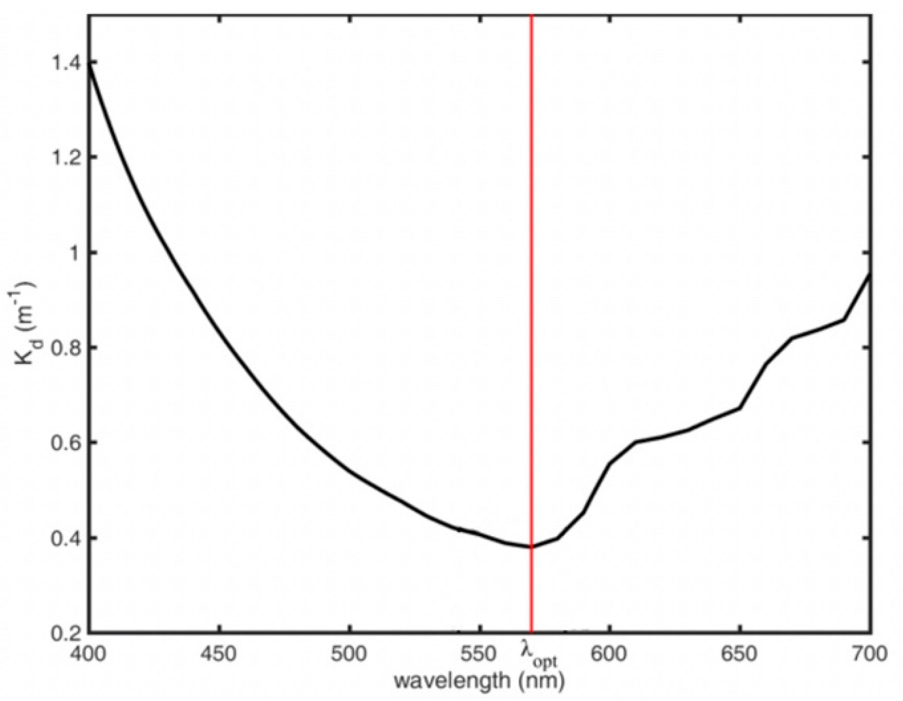
2.2. Definition of the Optimal Wavelength and the Detectable Depth

Some basic information is presented here before defining the optimal wavelength and the detectable depth as follows.
Based on the analysis of lidar received signals from current research results [6,13,17], the attenuation coefficient for lidar in water ( K lidar ) is the diffuse attenuating coefficient ( K d ) or the collimated attenuation coefficient (c), depending on the field of view and the detection height. The detection capability of lidar hardware is often evaluated on the number of attenuating lengths (ALs) achieved. The AL is defined in Equation (1); one AL is equivalent to the K lidar value multiplied by the geometry depth which equals to 1. Therefore, the detection capability of a lidar system is N × AL (N represents a number) which indicates that the maximum geometry depth that can be detected is N / K lidar as shown in Equation (2):
K lidar × Z = 1
Z max = N / K lidar
Because we were mainly concerned with the influence of the optical properties of water on the detection ability of a lidar system, we assumed a fixed AL detection ability for the lidar system. According to reports from commercial bathymetric lidar, a maximum 4 AL can return a receivable signal [18,19]; therefore, a 4 AL detection ability for lidar systems was assumed in this research. In addition, the maximum depth of detection for lidar systems can be expressed as 4 / K lidar .
In addition, the K lidar value is a physical quantity that ranges from K d to c, and for K d and c, the value of K d is lower than the value of c. Therefore, to explore the maximum detection ability, we let K lidar equal K d to analyze the detectable depth and the optimal wavelength. Therefore, the wavelength corresponding to the minimum value of spectral K d ( K dmin ), as shown in Figure 1, can be used to represent the optimal wavelength for an oceanographical lidar system. It is noted that spectral K d in Figure 1 is only used as an illustration; it was measured in the coastal waters of the Yellow Sea in July 2018 under the support of the National Natural Science Foundation of China. After establishing the optimal wavelength, we can further use the value of K d at the optimal wavelength to analyze the detectable depth of the lidar system. Therefore, the optimal wavelength ( λ opt ) and the maximum detectable depth ( Z m a x 4 ) for a lidar system with a 4 AL detection ability can be defined using Equations (3) and (4) as follows:
K d ( λ opt ) = K dmin ( λ )
Z m a x 4 = 4 / K d ( λ opt )
In addition, in this research, the influence of the inelastic scattering, for instance, Raman scattering and fluorescence, and the polarization on the detection ability of an oceanographical lidar was omitted, because, for the impact of inelastic scattering, the attenuation in one specified band was included in the retrieved K d using a passive ocean color remote sensing technique as stated below, which was validated by extensive in situ measurements. As for the impact of polarization, it depends on the real design of the lidar hardware system. In this paper, the focus was on the maximum detection depth and premium detection wavelength; as for the detected parameter, it also depended on the real design of the lidar system and was beyond the scope of this research.

2.3. Method to Retrieve the Hyper-Spectral K d at the Global Scale

To obtain the value of spectral K d at the global scale, traditional passive multi-bands ocean color satellite MODIS data were used. The detailed flowchart for using MODIS data is shown in Figure 2. First, daily chlorophyll a (Chla), the absorption coefficient of detritus, and the colored dissolved organic matter at 443 nm ( a dg ( 443 ) ) and the backscattering coefficient at 555 nm ( b b ( 555 ) ) were retrieved from the daily remote sensing reflectance data from MODIS based on the color index algorithm (CIA) and the quasi-analytical algorithm (QAA), respectively [20,21]. Then, a simple averaging merging algorithm was used to obtain ten years of climatological monthly averaged data for Chla, a dg ( 443 ) and b bp ( 555 ) . The spectral dependence values a ph , a dg , and b bp from Lee et al. [22], Morel and Maritorena [23], Chen and Zhang [24] were used, respectively. The total absorption coefficient ( a ) was the sum of the absorption coefficient of pure water ( a w ), a ph and a dg ; and the total backscattering coefficient ( b b ) was the sum of the backscattering coefficient of pure water ( b bw ) and b bp . Once the spectral a and b b were obtained, a semi-analytical method shown in Equation (5) and developed by Lee et al. [25] for deriving the spectral diffuse attenuation coefficient ( K d ) was used. Ultimately, the climatological monthly averaged data for the spectral diffuse attenuation coefficient ( K d ) was obtained and the λ opt   and   Z m a x 4 values were established at the global scale according to Equations (3) and (4).
K d ( λ ) = ( 1 + 0.005 θ a ) a ( λ ) + ( 1 0.265 × b bw ( λ ) b b ( λ ) ) × 4.259 ( 1 0.52 e 10.8 a ( λ ) ) b b ( λ )
where θ a represents the solar zenith angle.

3. Results

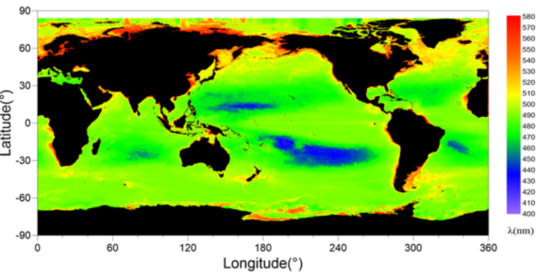
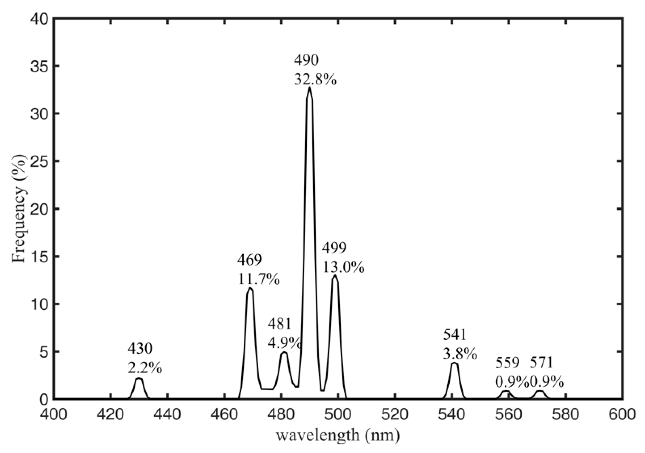
3.1. Distribution of the Optimal Wavelength at the Global Scale

Figure 3 shows the wavelength distribution at which the value of K d is a minimum. For convenience, the wavelength is represented by its color (meaning the blue band is denoted by a blue color and the green band is denoted by a green color). The optimal wavelengths corresponding to a minimum K d value range from the blue to the green bands. The optimal wavelengths for the open ocean range from 420 to 510 nm and from 520 to 580 nm for coastal waters. To further illustrate the optimal wavelength in different regions, the frequency distribution of the optimal wavelengths is shown in Figure 4. As shown, the optimal wavelengths are approximately 430, 469, 481, 490, 499, 541, 559, and 571 nm, respectively. For 32.8% of the global oceans, the optimal wavelength is 490 nm. In addition, the optimal wavelengths ranged from 460 to 510 nm regions for 80% of the global oceans.

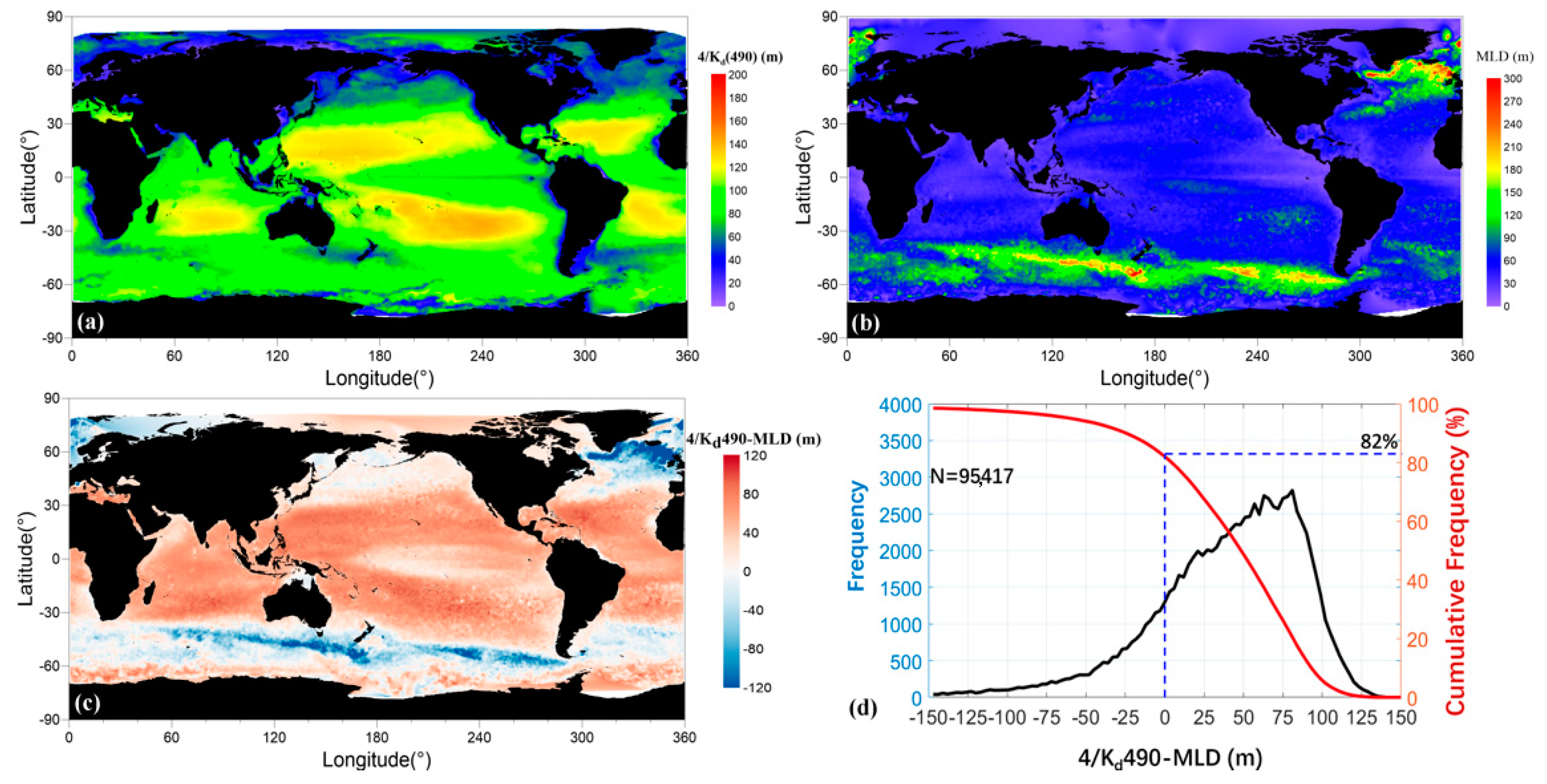
3.2. Distribution of the Maximum Detectable Depth of Lidar at the Global Scale and its Relationship with the Upper Mixed Layer Depth

Because the ultimate objective of using lidar is to detect the vertical structure of the water column, the detectable depth and whether lidar can penetrate the upper mixed layer to obtain information, such as depth, are primary concerns. In this section, we further analyze the detectable depth using the optimal wavelength 490 nm. The maximum detectable depth should be estimated from the corresponding optimal wavelength for different regions, but not all of the wavelengths established in Section 3.1 can be determined for the current lidar system. Here, we used the 490 nm wavelength which is suitable for most of the oceans as a proxy to discuss the relationship between the detectable depth of oceanographic lidar and the upper mixed layer depth which is established by the Argo data [26].
Figure 5a shows the distribution of the maximum detectable depth using 490 nm. In oligotrophic oceanic waters, the detectable depth can reach up to 110–150 m; in usual oceanic waters, it can reach up to 60–100 m; and in eutrophic coastal waters, the detectable depth is less than 50 m. The frequency and cumulative frequency distributions of the detectable depth shown in Figure 5 show that, for 95% of the global waters, the detectable depth is greater than 40 m, and for 60% of the global waters, the detectable depth is greater than 80 m. Figure 5b shows the distribution of the mixed layer depth at the global scale. In addition, Figure 5c shows the difference between the maximum detection depth and the MLD. For most of the global ocean, 490 nm lidar can penetrate the upper mixed layer and detect the region below it, especially in mid-latitude regions. The regions in which lidar cannot penetrate are mainly located at high latitudes where there is strong vertical mixing. In addition, Figure 5d shows that the lidar system with a 490 nm wavelength can obtain water profile information under the upper mixed layer for 80% of global waters. It is noted that there are 623,520 points for the data from satellite at the global scale, but for data from Argo, there only 95,417 points.

4. Discussion

In the section above, the optimal wavelength, the maximum detectable depth, and the relationship between the maximum detectable depth and the upper mixed layer depth are determined based on the assumption that the lidar system has a fixed detection ability of 4 AL. However, not only are several optimal wavelengths difficult to determine for current lidar systems but also current lidar systems cannot always detect 4 AL, especially when they are spaceborne because of the large attenuation created by long distances and the effect of the atmosphere.
In this section, we further discuss the factors that influence the detection ability, including the band difference, and the detection ability at different ALs, respectively.

4.1. Comparison of the Performances of Oceanographic Lidar Systems with Different Wavelengths

To discuss the influence of different wavelengths on the detection ability, three typical wavelengths that can be currently determined were selected: 490 nm (the optimal wavelength for the majority of the ocean), 455 nm (developing laser), and 532 nm (mature laser).
Figure 6a,b show the differences in the detectable depth between 455 and 532 nm and 490 and 532 nm, respectively. The detectable depth was estimated based on the same assumption that the laser detection system could have a detection ability of 4 AL. The warm color (red) represents the positive values (the detectable depth at 455 nm is greater than that at 532 nm) and vice vasa. Figure 6a shows that, for most of the ocean, the difference is positive except for the regions in high latitudes. This illustrates that using the 455 nm as the detection wavelength is preferable to using the 532 nm. Similarly, Figure 6b shows that, for most of the ocean, the difference is positive except for in several small regions located in coastal waters. Therefore, we conclude that using 490 nm as the detection wavelength is better than using the 455 and 532 nm wavelengths. The statistical results shown in Figure 6c,d further illustrate that, compared with the 532 nm wavelength, using the 455 nm wavelength improves the detectable depth for 75% of the global oceans and the average improvement in this depth is approximately 20 m. In addition, using 490 nm as the detection wavelength improved the detection depth for 90% of the global oceans, with an average improvement of approximately 30 m. The above analysis further illustrates that 490 nm is the optimal wavelength for oceanographic lidar. This section describes the differences in the detection ability at different bands, with the assumption of an oceanographic lidar system with a single wavelength. If possible, the best configuration for oceanographic lidar is one in which a laser with multiple wavelengths and the ability to switch wavelengths is used as described in Section 3.1.

4.2. Impact of Different Detection Ability of Lidar System on Detection Performance

The analyses of the maximum detectable depth in this research were all based on the assumption that the lidar system had a detection ability of 4 AL. In this section, the influence of the detection ability under different AL is discussed Figure 5c and Figure 7 show the difference in the detectable depths under a 4, 3, and 2 AL detection ability using the optimal wavelength of 490 nm. For a wavelength of 490 nm, the detection ability decreased significantly as the detectable depth decreases, but the lidar could still penetrate the upper mixed layer for most of the global oceans, especially in the middle and low latitudes. Therefore, the degradation of the detection ability for lidar systems has a weak influence on the profile detection of water columns and the detection in the upper mixed layer at the global scale.

5. Conclusions

In this research, the optimal wavelength for detecting global-scale characteristics of the water column profile using a lidar system was determined based on the inherent optical properties of water. In addition, assuming that the lidar system has optimal detection characteristics in its hardware design, the maximum detectable depth using the established optimal wavelength was analyzed and compared with the mixed layer depth measured by Argo data at the global scale. In addition, the factors that influence the detection capabilities at different ALs, including band difference, and detection ability were also discussed. The conclusions are as follows:
(a)
The optimal wavelengths for oceanographic lidar systems are those between the blue and green bands. For the open ocean, the optimal wavelengths are between 420 and 510 nm, and for coastal waters, the optimal wavelengths are between 520 and 580 nm. A lidar system with multiple bands is the best configuration for obtaining the best detection at the global scale. In addition, if an oceanographic lidar system with a single band is used at the global scale, a 490 nm wavelength is recommended.
(b)
Using the 490 nm band, a lidar system with four attenuating length detection methods can penetrate the mixed layer of over 80% of global waters.
In addition, the maximum detectable depth at the global scale analyzed above was measured by passive ocean color satellites. The data obtained from passive ocean color sensors is the weighted integral signal from the first attenuating depth [27] and the values are approximately equal to those of the surface waters. However, if the vertical profile distribution (VPD) is inhomogeneous, the detection ability of an oceanographic lidar system will be affected. The results of this research are based on the assumption of vertically homogeneous values for a and b b ; however, the values of a and b b and K d are depth-inhomogeneous and will influence the actual detection ability of the lidar system. Generally, for open oceans, the variability in the optical properties is mainly dominated by phytoplankton and their appendants [28,29]. The vertical profile of phytoplankton varies among regions and within the same region, and large changes can be observed at different time scales [30]. We also performed this analysis using global Bio-Argo data (not shown here). Therefore, a further analysis of the impact of a vertically inhomogeneous profile on the detection ability of oceanographic lidar systems will be conducted in the future as well as the inelastic scattering, polarization, and atmosphere for the future space-borne oceanographic lidar.

Author Contributions

Conceptualization, T.Z., G.C. and J.T.; Data curation, C.X.; Formal analysis, S.C.; Methodology, S.C.; Visualization, C.X.; Writing—original draft, S.C.; Writing—review & editing, T.Z. and L.H.

Funding

Financial support for this study was provided by the Marine S&T Fund of Shandong Province for Pilot National Laboratory for Marine Science and Technology (Qingdao) (No.2018SDKJ0102-7), the National Key R&D Program of China under Grant 2016YFC1400900, 2016YFC1400904, and the National Natural Science Foundation of China (NSFC) under grant numbers 61705211.

Acknowledgments

We are grateful to the NASA Ocean Biology Processing Group for providing passive ocean color satellite data. Thanks to the hard-working people who maintain the website http://www.oao.obs-vlfr.fr/web/index.php for providing the Bio-Argo dataset. The comments from anonymous reviewers are also much appreciated.

Conflicts of Interest

The authors declare no conflict of interest.

References

  1. Brainerd, K.E.; Gregg, M.C. Surface mixed and mixing layer depths. Deep Sea Res. 1995, 42, 1521–1543. [Google Scholar] [CrossRef]
  2. De Boyer Montégut, C.; Madec, G.; Fischer, A.S.; Lazar, A.; Iudicone, D. Mixed layer depth over the global ocean: An examination of profile data and a profile-based climatology. J. Geophys. Res. 2004, 109, C12003. [Google Scholar] [CrossRef]
  3. Morel, A.; Berthon, J. Surface pigments, algal biomass profiles, and potential production of the euphotic layer: Relationships reinvestigated in view of remote-sensing applications. Limnol. Oceanogr. 1989, 34, 1545–1562. [Google Scholar] [CrossRef]
  4. Collister, B.L.; Zimmerman, R.C.; Sukenik, C.I.; Hill, V.J.; Balch, W.M. Remote sensing of optical characteristics and particle distributions of the upper ocean using shipboard lidar. Remote Sens. Environ. 2018, 215, 85–96. [Google Scholar] [CrossRef]
  5. Hair, J.; Hostetler, C.; Hu, Y.; Behrenfeld, M.; Butler, C.; Harper, D.; Hare, R.; Berkoff, T.; Cook, A.; Collins, J. Combined atmospheric and ocean profiling from an airborne high spectral resolution lidar. EPJ Web Conf. 2016, 119, 22001. [Google Scholar] [CrossRef]
  6. Churnside, J.H. Review of profiling oceanographic lidar. Opt. Eng. 2013, 53, 051405. [Google Scholar] [CrossRef]
  7. Hu, Y.; Behrenfeld, M.; Hostetler, C.; Pelon, J.; Trepte, C.; Hair, J.; Slade, W.; Cetinic, I.; Vaughan, M.; Lu, X.; et al. Ocean lidar measurements of beam attenuation and a roadmap to accurate phytoplankton biomass estimates. EPJ Web Conf. 2016, 119, 22003. [Google Scholar] [CrossRef]
  8. Behrenfeld, M.J.; Hu, Y.; O’Malley, R.T.; Boss, E.S.; Hostetler, C.A.; Siegel, D.A.; Sarmiento, J.L.; Schulien, J.; Hair, J.W.; Lu, X.; et al. Annual boom–bust cycles of polar phytoplankton biomass revealed by space-based lidar. Nat. Geosci. 2017, 10, 118–122. [Google Scholar] [CrossRef]
  9. Chen, G.; Tang, J.; Zhao, C.; Wu, S.; Yu, F.; Ma, C.; Xu, Y.; Chen, W.; Zhang, Y.; Liu, J.; et al. Concept Design of the “Guanlan” Science Mission: China’s Novel Contribution to Space Oceanography. Front. Mar. Sci. 2019, 6, 194. [Google Scholar] [CrossRef]
  10. Jamet, C.; Ibrahim, A.; Ahmad, Z.; Angelini, F.; Babin, M.; Behrenfeld, M.J.; Boss, E.; Cairns, B.; Churnside, J.; Chowdhary, J.; et al. Going Beyond Standard Ocean Color Observations: Lidar and Polarimetry. Front. Mar. Sci. 2019, 6, 251. [Google Scholar] [CrossRef]
  11. Behrenfeld, M.J.; Hu, Y.; Hostetler, C.A.; Dall’Olmo, G.; Rodier, S.D.; Hair, J.W.; Trepte, C.R. Space-based lidar measurements of global ocean carbon stocks. Geophys. Res. Lett. 2013, 40, 4355–4360. [Google Scholar] [CrossRef]
  12. Churnside, J.; Hair, J.; Hostetler, C.; Scarino, A. Ocean Backscatter Profiling Using High-Spectral-Resolution Lidar and a Perturbation Retrieval. Remote Sens. 2018, 10, 2003. [Google Scholar] [CrossRef]
  13. Bogucki, D.J.; Spiers, G. What percentage of the oceanic mixed layer is accessible to marine Lidar? Global and the Gulf of Mexico prospective. Opt. Express 2013, 21, 23997–24014. [Google Scholar] [CrossRef] [PubMed]
  14. Gray, D.J.; Anderson, J.; Nelson, J.; Edwards, J. Using a multiwavelength LiDAR for improved remote sensing of natural waters. Appl. Opt. 2015, 54, 232–242. [Google Scholar] [CrossRef]
  15. Ocean Color Web. Available online: https://oceancolor.gsfc.nasa.gov/ (accessed on 18 October 2019).
  16. ARGO GDAC global distribution—FTP Directory Listing—Ifremer. Available online: ftp://ftp.ifremer.fr/ifremer/argo (accessed on 18 October 2019).
  17. Zege, E.P.; Katsev, I.L.; Prikhach, A.S. Inversion of Airborne Ocean LIDAR Waveforms. In Proceedings of the 22nd Internation Laser Radar Conference, Matera, Italy, 12–16 July 2004; Available online: http://www.researchgate.net/profile/Eleonora_Zege/publication/234256823_Inversion_of_Airborne_Ocean_LIDAR_Waveforms/links/09e4151126723b24f4000000.pdf (accessed on 18 October 2019).
  18. Teledyne Optech. CZMIL-Nova Coastal Zone Mapping and Imaging LiDAR. Available online: http://info.teledyneoptech.com/acton/attachment/19958/f-02c3/1/-/-/-/-/CZMIL-Nova-Intro-Brochure-150626-WEB.pdf (accessed on 18 October 2019).
  19. Airborne Hydrography. A. B. Leica AHAB “HawkEye III Topographic & Bathymetric LiDAR System”. Available online: http://www.airbornehydro.com/sites/default/files/Leica%20AHAB%20HawkEye%20DS (accessed on 18 October 2019).
  20. Hu, C.; Lee, Z.P.; Franz, B. Chlorophyll a algorithms for oligotrophic oceans: A novel approach based on three-band reflectance difference. J. Geophys. Res. Ocean. 2011, 117, C01011. [Google Scholar] [CrossRef]
  21. Lee, Z.P.; Carder, K.L.; Arnone, R. Deriving inherent optical properties from water color: A multiband quasi-analytical algorithm for optically deep waters. Appl. Opt. 2002, 41, 5755–5772. [Google Scholar] [CrossRef]
  22. Lee, Z.P.; Carder, K.L.; Peacock, T.G.; Davis, C.O.; Mueller, J.L. Method to derive ocean absorption coefficients from remote-sensing reflectance. Appl. Opt. 1996, 35, 453–462. [Google Scholar] [CrossRef]
  23. Morel, A.; Maritorena, S. Bio-optical properties of oceanic waters: A reappraisal. J. Geophys. Res. Ocean. 2001, 106, 7163–7180. [Google Scholar] [CrossRef]
  24. Chen, S.; Zhang, T. Evaluation of a QAA-based algorithm using MODIS land bands data for retrieval of IOPs in the Eastern China Seas. Opt. Express 2015, 23, 13953–13971. [Google Scholar] [CrossRef]
  25. Lee, Z.P.; Hu, C.; Shang, S.; Du, K.; Lewis, M.R.; Arnone, R.; Brewin, R.J. Penetration of UV-visible solar radiation in the global oceans: Insights from ocean color remote sensing. J. Geophys. Res. 2013, 118, 4241–4255. [Google Scholar] [CrossRef]
  26. Holte, J.; Talley, L.D.; Gilson, J.; Roemmich, D. An Argo mixed layer climatology and database. Geophys. Res. Lett. 2017, 44, 5618–5626. [Google Scholar] [CrossRef]
  27. Hostetler, C.A.; Behrenfeld, M.J.; Hu, Y.; Hair, J.W.; Schulien, J.A. Spaceborne Lidar in the Study of Marine Systems. Annu. Rev. Mar. Sci. 2018, 10, 121–147. [Google Scholar] [CrossRef] [PubMed]
  28. Morel, A. Optical modeling of the upper ocean in relation to its biogenous matter content (Case I waters). J. Geophys. Res. 1988, 93, 10749–10768. [Google Scholar] [CrossRef]
  29. Gordon, H.R.; Morel, A. Remote Assessment of Ocean Color for Interpretation of Satellite Visible Imagery: A Review; Springer: New York, NY, USA, 1983. [Google Scholar]
  30. Lavigne, H.; Dortenzio, F.; Dalcala, M.R.; Claustre, H.; Sauzede, R.; Gacic, M. On the vertical distribution of the chlorophyll a concentration in the Mediterranean Sea: A basin scale and seasonal approach. Biogeosciences 2015, 12, 5021–5039. [Google Scholar] [CrossRef] [Green Version]
Figure 1. Definition of the optimal wavelength.
Remotesensing 11 02705 g001
Figure 2. Flowchart for retrieving spectral K d using MODerate Imaging Spectroradiometer (MODIS) data.
Remotesensing 11 02705 g002
Figure 3. Spatial distribution of the optimal wavelengths at the global scale.
Remotesensing 11 02705 g003
Figure 4. Frequency distribution of the wavelength corresponding to a minimum value of K d .
Remotesensing 11 02705 g004
Figure 5. Distribution of the maximum detectable depth for oceanographic lidar (a), the upper mixed layer depth (MLD) (b), the difference between the maximum detection depth and the MLD (c), and the frequency distribution of the difference between the maximum detection depth and the MLD (d).
Remotesensing 11 02705 g005
Figure 6. Global distribution of the maximum detection depth difference (a,b) and the frequency and cumulative frequency distributions of the differences (c,d) following the assumption that the optimal detection for lidar is 4 AL between 455 and 532 nm (a,c) and 490 and 532 nm (b,d), respectively.
Remotesensing 11 02705 g006
Figure 7. Comparison of detection performance at different detection abilities of a lidar system under 3 AL (a) and 2 AL (b).
Remotesensing 11 02705 g007

