Assessment of Phytoecological Variability by Red-Edge Spectral Indices and Soil-Landscape Relationships

Abstract

There is a relation of vegetation physiognomies with soil and geological conditions that can be represented spatially with the support of remote sensing data. The goal of this research was to map vegetation physiognomies in a mountainous area by using Sentinel-2 Multispectral Instrument (MSI) data and morphometrical covariates through data mining techniques. The research was based on red-edge (RE) bands, and indices, to classify phytophysiognomies at two taxonomic levels. The input data was pixel sampled based on field sample sites. Data mining procedures comprised covariate selection and supervised classification through the Random Forest model. Results showed the potential of bands 3, 5, and 6 to map phytophysiognomies for both seasons, as well as Green Chlorophyll (CLg) and SAVI indices. NDVI indices were important, particularly those calculated with bands 6, 7, 8, and 8A, which were placed at the RE position. The model performance showed reasonable success to Kappa index 0.72 and 0.56 for the first and fifth taxonomic level, respectively. The model presented confusion between Broadleaved dwarf-forest, Parkland Savanna, and Bushy grassland. Savanna formations occurred variably in the area while Bushy grasslands strictly occur in certain landscape positions. Broadleaved forests presented the best performance (first taxonomic level), and among its variation (fifth level) the model could precisely capture the pattern for those on deep soils from gneiss parent material. The approach was thus useful to capture intrinsic soil-plant relationships and its relation with remote sensing data, showing potential to map phytophysiognomies in two distinct taxonomic levels in poorly accessible areas.

1. Introduction

Tropical regions in mountainous relief are considered of great importance for the conservation of natural resources, presenting high biological diversity and endemism index, propitiated by the variety of environments associated to abiotic and biotic factors [1,2,3]. Some of these regions present a specific physiognomy called a nebular forest. These are areas with climatic and topographic conditions favorable to the constant presence of fog. The areas present well-developed natural forests, because they remain frequently enveloped in fog and clouds, and are generally called cloud or nebular forests [3,4]. These forests account for only 2.5% of the total area of tropical forests in the world, with an overall surface area of approximately 380,000 km² [5].

In Brazil, nebular forests are located mainly at high altitudes along the Serra do Mar formation in the states of Santa Catarina, Paraná, São Paulo, and Rio de Janeiro. These forests are also found in small stretches of the Mantiqueira ridge of Minas Gerais, and in the high plateaus and mountains of the Amazon [1,6]. The upper montane vegetation in the Southeastern region of Brazil is constituted by a vegetative mosaic composed by forest and field formations, which vary according to the geographic region and altitude [1]. The heterogeneity of vegetation types is strongly related to the topographic irregularity and altitudinal gradients ruling the temperature conditions, air humidity, water availability, exposure to winds, and soil depth and drainage conditions [7,8,9,10]. Santos et al. (2011) [11] and Streher and Silva (2015) [12] observed changes in vegetation phytophysiognomies at the Meridional Espinhaço ridge, also in Minas Gerais State, due to the topographic and edaphic diversity. The diversity of phenological patterns for tropical vegetation have been widely reported as savanna and humid forests [13,14].

The nebular forests also promote additional water entry into the ecosystem through hidden precipitation, which is the horizontal interception of atmospheric clouds through trees and shrubs, subsequently falling to the forest floor [15]. Thus, for these localities, the capture of water from the atmosphere constitutes an important process in the hydrological cycle of the regional watersheds [3,4,15].

In this context, the Ibitipoca State Park (ISP) represents an important forested area at the Southeastern region of Brazil specifically on the south of Minas Gerais State. The ISP has been one of the most visited parks of the country, totaling 95,000 in 2015, according to Forests State Institute of Minas Gerais (IEF-MG). It is currently facing new rules of visitation targeting environmental preservation and visitor safety [16], by reducing the number of daily visitors by half, according to the Forest State Institute of Minas Gerais (IEF-MG). The ISP presents a remarkable geology consisting of Proterozoic metasedimentary rocks presenting rupitle-ductile tectonic features, forming a hilly mountain chain over folded quartzite, with several caves, and waterfalls [17]. This geological context drives the relationship with soil formation and phytophysiognomies, which thus presents a wide variability of natural vegetation types [2]. Considering the specificities of the vegetation at the ISP, several authors adopted a flexible vegetation classification system that could accommodate all the phytophysiognomies of the region, as well as the environmental characteristics at the more detailed taxonomic levels [1,2,3].

The identification of homogenous regions with data mining tools is commonly done by quantitative interpretation from products derived from remote sensing images (orthophotos or orbital data), considering the similarities between the features and the neighborhood [18], allowing to reduce the time and cost when compared with vectorized vegetation maps, based only on field-collected data and photointerpretation [19,20]. These techniques can also be useful in areas with limited access, as prevalent in this study area.

A further problem facing researchers studying environmental conservation relates to the lack of accessibility. Addressing this issue, authors such as Cambule et al. (2013), Minasny and McBratney (2006), Roudier et al. (2012) [21,22,23] proposed a methodology for sampling in areas that have limited access. Carvalho Junior et al. (2014) [24] applied the methodology suggested by Minasny and McBratney (2006) [22], to assess soil property variation with success, known as Conditioned Latin Hypercube sampling (cLHS). A similar procedure was used by Costa et al. (2018) [25] in Itatiaia National Park also in the Southeastern region of Brazil, focused on mapping the environmental vulnerability.

Nowadays, several remote sensing datasets exist that can be used to define vegetation types and soil properties. Among them, the Sentinel-2 Multispectral Instrument (MSI) derived indices show the highest potential to classify vegetation types and phenological differences, since it highlights prominent spectral features of vegetation due to the segmentation of the red spectral band, when compared with Landsat data, decompounding four bands in the red interval (705, 740, 783, and 865 nm). This spectral interval is defined as red-edge (RE). The RE comprises a spectral range composed of bands located between the maximum red absorption and the high reflectance of the near-infrared (NIR). Fernandez-Manso et al. (2016), Frampton et al. (2013), and Clevers and Gitelson (2012) [26,27,28] proposed several indices derived from spectral bands at the RE to study canopy chlorophyll content and leaf area index.

The use of remote sensing data is justified to map vegetation at more detailed scales, since at the macroscale (regional and continental) the vegetation types are mainly controlled by climate conditions [29]. However, the heterogeneity of vegetation at detailed scales can be highly dependent on pedological control due the availability of water and nutrients [30]. The innovation of this study lies in the use of RE indices and the Sentinel-2 MSI bands, as well as in quantitatively explaining the relation among vegetation physiognomies and soil-landscape patterns, aiding taxonomic classification at more detailed levels, where climate conditions do not explain the physiognomy variability. The justification to use more detailed taxonomic classification adapted to the region was based on the relation between phytophysiognomies, which is directly related to soil properties on a local scale, especially soil depth in the case of the ISP.

Following the increased trend of remote sensing data availability, the phenological remote sensing-based studies are also increasing, as are the different time-scale approaches according to the sensors used [12,20,31,32,33]. Inspired by the challenge to map vegetation types in a complex relief by using remote sensing data and data mining tools, this research aims to classify vegetation types at two taxonomic levels, according to Oliveira Filho (2009) [1].

The objective of this study was thus to analyze the spatial distribution of different phytophysiognomies, in a heterogeneous landscape with a complex relief due to strong geological control over morphogenetic and pedogenetic processes, by using field-collected data, landscape information, and remote sensing data, particularly, red-edge indices for the ISP, in Minas Gerais, Brazil.

2. Materials and Methods

2.1. Study Area and Phytoecological Relationships

The ISP is located between coordinates 21°40′15”, 21°43′30” S, and 43°52′35”, 43°54′15” W, inside the complex relief of Meridional Mantiqueira ridge, with elevation ranging between 1200 and 1800 m (Figure 1).

The climate is classified as Cwb, according to Köppen classification with cold and dry winters, and warm and wet summers, with an annual average temperature of 18.9 °C [34]. The study of Rodela and Tarifa (2002) [35] defined three climatic compartments, directly related to the elevation (Figure 2a). A geographic information system (GIS) was used to obtain numerical surface models to represent morphometrical parameters such as elevation and slope, derived from a hydrological consistent digital elevation model (DEM). The hydrologically consistent elevation model was used to derive land surface attributes, such as slope, Geomorphons, Landforms, and for this reason a sequence of intermediate layers (flow accumulation, flow direction, and sinks) were calculated to detect spurious depressions.

All these analyses were done within the park boundary (available on the website of the National Register of Conservation Units—CNUC) and from the BIASFORTES topographic chart (SF23-XC-VI), on a 1:50,000 scale, available from the Brazilian Army Geographic Database (BDGEx). The DEM, with a spatial resolution of 10 m, was obtained by interpolation in the ArcGIS Desktop v.10.3 (TopotoRaster) using as input data elevation points and 20 m contour lines. Spurious depressions resulting from the interpolation procedure were corrected to obtain a hydrologically consistent model (Figure 2b) using the Hidrology toolbox in ArcGIS. Products such as synthetic shading (hillshade), and slope (Figure 2c) were derived from the consistent hydrological DEM. In addition, Landforms and Geomorphons maps were calculated from the DEM, in SAGA-GIS [36] and GRASS-GIS [37] respectively. Both maps were used to represent geomorphological aspects of the area in more detail, since geology and soil maps are only available at coarse scales. Previous studies by the authors in the area (unpublished) detected a direct correlation among these landscape attributes and soil properties and classes. The parameters used to create the Landforms map were the default (radius A = 0, 100 m; radius B = 0, 1000 m; no distance weighting). The Geomorphon map was defined with 30 cells search radius and the default relief threshold value (1°), or flatness threshold (difference, in degrees, between zenith and nadir line-of-sight in the horizontal direction). More detail about Geomorphon landform classification is given by Jasiewicz and Stepinski (2013) [38].

According to the World Reference Base [39], mineral soils in the park are mostly sandy soils, including Regosols, Arenosols, and Podzols, overlying Quartzite rocks. However, Cambisols with micaceous minerals overly punctual Gneiss outcrops in the central and southern portion of the park, while Histosols are found at high elevations (Figure 2d, [40]). Nummer (1991) [17] and Pinto (1991) [41] defined two main tectonostratigraphic units in the ISP area, comprising quartzite (with micaceous or/and coarse granulated facies), and gneiss (weathered and punctual occurrences at the central and southern portions of the park) presented in Figure 2e. Figure 2f presents the detail field sampling points for vegetation, soil, and geology in November 2018 and April 2019.

The field campaigns were performed by using a methodology adequate to studies in poorly accessible areas. The selection of 30 sampling points was performed through the cLHS technique proposed by Minasny and McBratney (2006) and Roudier et al. (2012) [22,23]; where a sample set was defined by considering the feasibility of accessing a representative sample site. The algorithm was executed in the R program through the cLHS package. To set the parameters for conditioning the sampling scheme, an accessible area was defined by a buffer of 30 m around mapped trails, the number of sample points (30), correlation and data weight (0.5 and 1.0 respectively), and the number of iterations (10,000).

Landsat 8 images (sensor OLI) with 30 m spatial resolution (September 14, 2017), particularly bands 4, 5, and 6 (visible + infrared) were used to select the field sample points by cLHS stratification. The image corrections routine applied was the same of Sentinel-2 MSI, described in Section 2.3. Landsat 8 was used in the preliminary phase to guide the field campaign, despite the poorer spatial and spectral resolution of Landsat 8, compared with Sentinel-2 MSI. All images (Landsat 8 and Sentinel-2 MSI) were acquired from the USGS website [42]. Additionally, the elevation (DEM) and slope were considered to distinguish different landscape conditions. More details about this technique are given by Cambule et al. (2013) [21] and Costa et al. (2019) [25].

The field campaigns were executed in 2018 and 2019, during the wet and dry seasons by a multidisciplinary team with a pedologist, geologists, and forest engineers to classify the vegetation and to support the inferences about the landscape conditions defining the distinct phytophysiognomies at the sample sites.

2.2. Taxonomic Classification of Phytophysiognomies

The taxonomic classification system adopted in this study was proposed by Oliveira-Filho (2009) adapted to tropical South American and subtropical cis-Andean regions [1]. The classification was used due to it being better adapted to environments with high heterogeneity especially in plant communities such as in the ISP region, to grasp with data mining techniques (Random Forest model). In this system, it is possible to combine several hierarchical attributes to meet a wide variety of spatial scale and respective levels of detail [1,2].

The first hierarchical attributes observed for the phytophysiognomies classification are the climatic regime, altitude, and thermic domain. The ISP occurs at altitudes higher than 1100 m and is located between 12° and 24° South, conferring the classification of “Tropical Upper Highlands” to the thermic domain. The climatic regime of all ISP vegetal formations was classified as “Cloud” because they occur in areas where the horizontal precipitation is higher than 30% and present less than 80 days of drought per year. Foliar Renewal was another attribute to classify vegetation types, where two classes were detected in this study. The phytophysiognomies that present between 30% and 60% of leaf fall in the dry season was classified as “Semi-deciduous”, while those where less than 30% of the leaf mass is released in the same season are called “Perennial”. Among the phytophysiognomies evaluated in this study, only the savannas belong to the “Semi-deciduous” class [2]. The last attribute evaluated in the field study was the Substrate where the phytophysiognomies were established at more detailed levels (Fifth taxonomic level). Substrates with soil depth ≥0.5 m were referred to as “Deep soils” and “Shallow soils” were <0.5 m, while bare and fragmented rocks with sediments were classified as “Rocky” [1].

At the ISP area, the general phytophysiognomies, according to [1], comprise Bushy grassland; Broadleaved scrub; Shrubland savanna; Parkland savanna; Broadleaved dwarf-forest; and Broadleaved forest. The general phytophysiognomies, the detailed classification and the number of sample sites for each class are presented in

Table 1. Phytophysiognomies considered at the two taxonomic levels [1].

Physiognomies (1st)	Description of General Taxonomic Level	Attribute (5th) *	N **
Broadleaved forest (FL)	The trees usually have broad leaves and make up a canopy between 5 and 30 m in height, although the emergent trees may be sparsely populated. Climbers and epiphytes are very frequent in this forest formation.	Broadleaved forest over deep soils (FLd)	1
		Broadleaved forest over shallow soils (FLs)	1
Broadleaved dwarf-forest (NL)t	Nearly all trees are broadleaved and form a low canopy, between 3 and 5 m in height. Scattered taller trees may emerge from the canopy. Climbers, epiphytes, and shrubs may be relevant.	Broadleaved dwarf-forest over deep soils (NLd)	11
Parkland savanna (SL)	The woody biomass is predominant, but the trees do not form a continuous canopy. The shrubs are abundant, and the bush forms an almost continuous vegetation cover.	Parkland savanna over shallow soils (SLs)	3
Shrubland savanna (SA)	The woody component is mainly composed of shrubs, while the trees are very rare. The shrub component is also significant and forms an almost continuous vegetation cover.	Shrubland savanna over shallow soils (SAs)	5
		Shrubland savanna and rocky outcrop (SAr)	2
Broadleaved scrub (AL)	Subshrubs and broadleaved shrubs form a nearly uniform vegetable mass, but without herbaceous plants coating the soil. There may be an expressive biomass of climbers and epiphytes.	Broadleaved scrub over shallow soils (ALs)	3
Bushy grassland (CL)	Broadleaved subshrubs, short-lived or perennial herbs make up discontinuous vegetable formation. Scattered shrubs and isolated trees may also occur.	Bushy grassland over shallow soils (CLs)	10

* Soil Depth: Shallow soils (<0.5 m) over rocks or rocky fragments. Tenuissólico; Deep soils (>0.5 m) over rocks or rocky fragments. Crassissólico. Rocky (rock outcrops). Rupícola. According to Oliveira-Filho (2009) [1]. N **: number of sample sites for each class identified along with field campaigns.

.

2.3. Remote Sensing Data and Processing

The images used to classify the vegetation phytophysiognomies were captured by the Sentinel-2A MSI (Multi-Spectral Instrument) sensor on September 6, 2017 (dry season) and Sentinel-2B MSI on December 10, 2017 (wet season) acquired from the ESA Sentinels Scientific Data Hub through the Earth Explorer platform [43]. Bands are available with geometric corrections (including orthorectification). Atmospheric correction was carried out using the AtmCor4MSI software [44] implemented based on the 6S radiative transfer code proposed by Vermote et al. (1997) [45]. For this correction a tropical gaseous atmosphere and a continental aerosol model was used, with a horizontal visibility of 18 km for the dry and wet season images. The resulting image was in surface reflectance stores of 16 bits. It calculates the atmospheric correction based on the radiance level in the sensor as a function of illumination, visualization, and atmospheric conditions on the day of capture. Next, spectral red-edge indices were computed (

Table 2. Vegetation indices derived from the Sentinel-2 MSI (Multi-Spectral Instrument) spectral bands.

Vegetation Index	Sentinel-2 MSI Bands	Reference
Normalized difference vegetation index (NDVI1)	$\frac{\left( {\rho }_{ band 8a} - {\rho }_{band 4}\right)}{\left( {\rho }_{ band 8a} + {\rho }_{band 4}\right)}$
Normalized difference vegetation index (NDVI2)	$\frac{\left( {\rho }_{ band 8} - {\rho }_{band 4}\right)}{\left( {\rho }_{ band 8} + {\rho }_{band 4}\right)}$	[27,46]
Soil-adjusted vegetation index (SAVI)	$\left(1+0.5\right)+\frac{\left( {\rho }_{ band 8} - {\rho }_{band 4}\right)}{\left( {\rho }_{ band 8} + {\rho }_{band 4}\right)}$	[45,47]
Inverted Red-Edge Chlorophyll Index (IRECI)	$\frac{\left( {\rho }_{ band 7} - {\rho }_{band 4}\right)}{\left( {\rho }_{ band 5} ÷ {\rho }_{band 6}\right)}$	[46]
Chlorophyll index (${\mathrm{Cl}}_{red-edge})$	$\frac{\left( {\rho }_{ band 7} \right)}{\left( {\rho }_{ band 5}\right)}-1$	[26,28]
Green chlorophyll index $({\mathrm{Cl}}_{green})$	$\frac{\left( {\rho }_{ band 7} \right)}{\left( {\rho }_{ band 3}\right)}-1$	[28]
Normalized difference vegetation index red-edge (NDVIre1)	$\frac{\left( {\rho }_{ band 8} - {\rho }_{band 5}\right)}{\left( {\rho }_{ band 8} + {\rho }_{band 5}\right)}$	[26]
Normalized difference vegetation index red-edge (NDVIre2)	$\frac{\left( {\rho }_{ band 8a} - {\rho }_{band 5}\right)}{\left( {\rho }_{ band 8a} + {\rho }_{band 5}\right)}$	[26]
Normalized difference vegetation index red-edge (NDVIre3)	$\frac{\left( {\rho }_{ band 8} - {\rho }_{band 6}\right)}{\left( {\rho }_{ band 8} + {\rho }_{band 6}\right)}$	[26]
Normalized difference vegetation index red-edge (NDVIre4)	$\frac{\left( {\rho }_{ band 8a} - {\rho }_{band 6}\right)}{\left( {\rho }_{ band 8a} + {\rho }_{band 6}\right)}$	[26]
Normalized difference vegetation index red-edge (NDVIre5)	$\frac{\left( {\rho }_{ band 8} - {\rho }_{band 7}\right)}{\left( {\rho }_{ band 8} + {\rho }_{band 7}\right)}$	[26]
Normalized difference vegetation index red-edge (NDVIre6)	$\frac{\left( {\rho }_{ band 8a} - {\rho }_{band 7}\right)}{\left( {\rho }_{ band 8a} + {\rho }_{band 7}\right)}$	[26]
Normalized Difference Red-edge (NDRE1)	$\frac{\left( {\rho }_{ band 6} - {\rho }_{band 5}\right)}{\left( {\rho }_{ band 6} + {\rho }_{band 5}\right)}$	[26,28]
Normalized Difference Red-edge (NDRE2)	$\frac{\left( {\rho }_{ band 7} - {\rho }_{band 5}\right)}{\left( {\rho }_{ band 7} + {\rho }_{band 5}\right)}$	[26,28]

).

The red-edge spectrum position is characterized by wavelet size. Further details regarding central wavelength, bandwidth, and resolution can be obtained from the USGS Website [42]

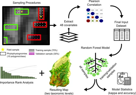
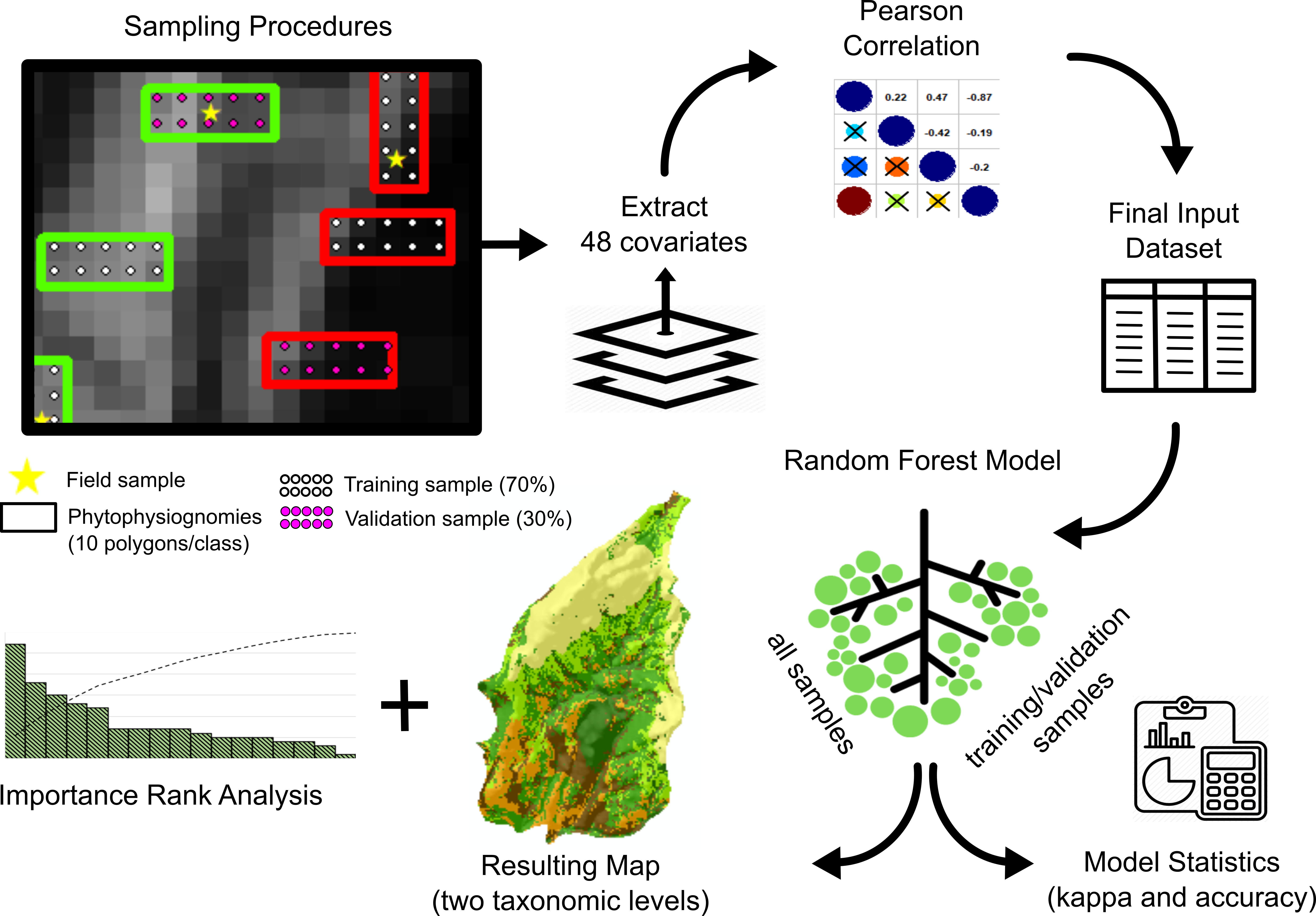
2.4. Supervised Phytophysiognomies Classification

Supervised classification [1] through the data mining algorithm and by adopting two taxonomic levels was used, to support the spatial analysis of vegetation distribution corresponding to Physiognomies (First Taxonomic Level) and Substrate Attributes (Fifth Taxonomic Level) and as presented in Table 1.

The collection of pixel samples to apply the supervised classification procedure was focused on capturing the different vegetation types (at two taxonomic levels) by using environmental variables as auxiliary information. Based on the field sampled points, polygons were created around the sample points to increase the number of samples used in the data mining steps, carefully respecting the main trend on the covariate’s values aiming to grasp the occurrence patterns of the different physiognomy types regarding spectral response and landscape conditions.

The stratification of phytophysiognomies types was performed based on field data and photointerpretation to delineate areas of homogeneous pixel tonality around the field data, that were separated first at the general taxonomic level, then at the detailed level. The sampling was done by visual inspection of the pixels around the sample sites, and by alternating the layers of the Sentinel bands and indices. At the end of this procedure 10 polygons, of approximately 1000 m² each, around field truth sample sites were created to represent the physiognomy types for each taxonomic level. As the physiognomy types occur disproportionately, some types were not adequately represented and were therefore selected manually. From those polygons, a portion were randomly selected and used to train (seven polygons) and validate (three polygons) the final model.

Pixel sampling was performed based on vectorized polygons, that were converted to point samples respecting the spatial resolution adopted for all layers used (10 m). The values of remote sensing indices and bands, and terrain covariates (DEM, Slope, Landforms, Geomorphons) were associated with each point data through Extract Values to Point toolbox in ArcGIS. Thematic maps on the coarse scale were not used as covariates in the predictive model, but the geomorphology represented by Geomorphons and Landforms categorical maps comprise geology and soil aspects due to the influence of relief resulting forms.

At the end of the sampling step from the total samples collected, 420 points and 560 points for the training dataset (for first and fifth taxonomic level, respectively), while 180 and 240 points for the validation dataset (for first and fifth taxonomic level, respectively) were selected, comprising a ratio of 70% and 30% respectively. The difference among the input samples for the different taxonomic levels was due to efforts to achieve sample balancing for each considered class, since for the detailed taxonomic level a largest number of classes has been designated.

After this procedure, Pearson’s correlation at 95% significance level was executed through “corrplot” package in the R environment [48] to aid the selection of potential covariates to use in data mining procedures through the Random Forest algorithm. The selection of covariates was performed in two steps: (i) remove from the input dataset the covariates highly correlated among each other, to avoid redundant predictors; (ii) assessment of the covariates’ importance aiming to reduce from the dataset the covariates with low importance to distinguish phytophysiognomies types by analyzing the contribution of each covariate to improve the classification accuracy. The final covariates dataset was obtained from these procedures and used in data mining steps, which comprises the statistical modelling of phytophysiognomies occurrence at the ISP area.

The data mining algorithm used to classify the vegetation types at the two detail levels was Random Forest model (RF), executed in R environment [48] through the “randomForest” package [49]. RF is a non-parametric technique developed as an extension of CART (Classification and Regression Trees) systems [50], to improve the performance of the predictors. To implement the RF model, three parameters are necessary: the number of trees in the forest (ntree); the minimum amount of data in each terminal node (nodesize); and the number of covariates used in each tree (mtry) [49]. The ntree value was set to the system default (500) [51]. The nodesize value was set to five for each terminal node, and the mtry value chosen in this study was according to Liaw and Wiener (2002) [49], which propose an amount corresponding to the root square of the total number of predictor variables.

The approach to mapping the vegetation have two instances. One is related to the covariate’s redundancy, aiming to simplify the model by removing the redundant covariates whenever possible according to the Occam’s razor statement, which preconizes that the simplest model should be chosen among others [52]. The covariates selection is performed by contrasting the correlation of each high related covariate, and all other covariates from the dataset, the variable with the highest significance is kept in the dataset [53]. For this reason the redundant covariates were firstly removed by correlation analysis and then the covariates with low importance were removed based on the rank provided by the Random Forest model that presents the contribution of each covariate on the model’s accuracy and Gini coefficient, which considers the node purity, i.e., the homogeneity from the covariates to each tree node. Those covariates that result in nodes with higher purity have a higher decrease in the Gini coefficient. The covariates used in the final model were selected from the correlation, and their importance to the classification procedure analyzed based on the rank provided by the RF model.

The assessment of the model’s performance was to evaluate the statistical indices and the coherence of the cartographical product to represent the vegetation types at the two distinct taxonomic levels. The statistical indices used were overall and kappa indices obtained from a confusion matrix, according to Monserud and Leemans (1992) [54]. All these procedures were performed firstly to the phytophysiognomies general level, then to the more detailed level according to Oliveira Filho (2009) [1], first and fifth taxonomic level, respectively. The flowchart below (Figure 3) summarizes the methodological procedures applied to classify the physiognomies at both taxonomic levels.

3. Results and Discussion

3.1. Phytophysiognomies and Landscape Relationships

From the input dataset with 48 covariates (four representing geomorphological aspects of landscape and 44 represented by the Sentinel-2 MSI bands, dry and wet seasons, and red-edge derived indices) a correlation analysis was performed with all the numerical models (continuum data), based on all samples collected to represent the physiognomy patterns. Pearson’s correlation allows a better understanding regarding the covariates which are highly correlated among each other and should be eliminated to produce a simpler explanatory model [52]. To perform this analysis, the categorical data, as Landforms and Geomorphons maps, were excluded once this analysis was correctly applied considering only the numerical models remaining at the correlation analysis (46 covariates).

Initially, 26 covariates were removed due to the redundancies with other potential predictors for the first taxonomic level and 25 were removed at the fifth taxonomic level, which is represented in Figure 4. When the correlation analysis was performed with the samples for the first taxonomic level, the same covariates were dropped due to the redundancy, except for the NDVIre1 from the dry season (September) that was kept at the fifth taxonomic level.

Among the covariates that were kept in the analysis, the bands 3 and 5 (for both seasons), and indices obtained from bands 6, 7, 8, and 8A calculated as [26] (Table 2), also for both seasons (NDVIre3, NDVIre4, NDVIre5, and NDVIre6).

The NDVI index calculated with band 5 (NDVIre2), IRECI, CLre, and NDRE according to Frampton et al. (2013) [27] (Table 2), for both seasons, were dropped due to the redundancy with other indices that present greater potential as a predictor, for example CLg and SAVI (Figure 4). At the end of the correlation analysis to the first taxonomic level 22 covariates remained, while to the fifth taxonomic level 23 were kept for classification procedures.

Posteriorly to the Pearson correlation analysis performed to avoid redundancy among covariates, the input dataset with the select samples and covariates was defined for each taxonomic level (Table 1), and the descriptive statistics to the samples from the fifth taxonomic level are presented in

Table 3. Descriptive statistics of the training and validation datasets from the pixels sampled at the fifth taxonomic level.

	Training Dataset (n = 560)					Validation Dataset (n = 240)
	Max.	Min.	Median	Avg.	SD	Max.	Min.	Median	Avg.	SD
DEM	1761	1300	1440	1468	38.31	1696	1352	1455	1471	38.35
Slope	70.559	2.418	18.737	22.37	4.73	50.928	1.953	27.971	27.25	5.22
B2_Dec	0.0759	0.0091	0.0284	0.0291	0.1706	0.0849	0.0086	0.0269	0.0844	0.2905
B3_Sep	0.1072	0.0083	0.0339	0.0357	0.1889	0.0915	0.0090	0.0295	0.0332	0.1823
B3_Dec	0.1093	0.0147	0.0493	0.0500	0.2237	0.1188	0.0301	0.0470	0.0494	0.2222
B5_Sep	0.1612	0.0404	0.0788	0.0787	0.2805	0.1302	0.0414	0.0720	0.0751	0.2740
B5_Dec	0.1457	0.0403	0.0894	0.0898	0.2997	0.1409	0.0648	0.0856	0.0880	0.2967
B6_Sep	0.2823	0.1093	0.1629	0.1693	0.4115	0.2621	0.1030	0.1617	0.1647	0.4058
B6_Dec	0.3762	0.0714	0.1925	0.2007	0.4480	0.3160	0.1325	0.1976	0.2049	0.4527
B8_Sep	0.4298	0.1102	0.2022	0.2135	0.4621	0.3426	0.1093	0.2032	0.2096	0.4578
CLg_Sep	29.1347	0.4948	4.2525	5.7762	2.4034	24.3490	1.2140	4.9070	6.3850	2.5269
NDVIre1_Sep	0.7524	0.0914	0.4253	0.4487	0.6698	0.7395	0.2192	0.4441	0.4653	0.6821
NDVIre3_Sep	0.2597	–0.0476	0.1119	0.1119	0.3345	0.2352	0.0158	0.1115	0.1169	0.3419
NDVIre4_Sep	0.1918	0.0768	0.1242	0.1263	0.3553	0.2033	0.0196	0.1279	0.1285	0.3585
NDVIre5_Sep	0.2243	–0.1227	0.0467	0.0450	0.2120	0.1532	–0.1136	0.4996	0.0474	0.2177
NDVIre6_Sep	0.1102	0.0134	0.0581	0.0594	0.2438	0.1029	0.0127	0.0587	0.0591	0.2431
NDVIre3_Dec	0.2405	–0.1681	0.1051	0.1065	0.3264	0.2111	–0.0092	0.1043	0.1098	0.3314
NDVIre4_Dec	0.1878	0.0891	0.1377	0.1398	0.3739	0.1872	0.0946	0.1372	0.1393	0.3732
NDVIre5_Dec	0.1299	–0.2267	0.0299	0.0247	0.1570	0.1214	–0.0943	0.0269	0.0256	0.1599
NDVIre6_Dec	0.1069	0.0235	0.0574	0.0583	0.2414	0.0331	0.0331	0.0540	0.0554	0.2354
SAVI_Dec	2.4500	1.7890	2.1450	2.1710	1.4734	2.4580	1.8650	2.1960	2.1950	1.4816

Max. = Maximum; Avg. = Average Min. = Minimum; SD = Mean Standard Deviation; Sep = September (dry season); Dec = December (wet season); DEM = Elevation; B03, B05, B06, and B08 = Selected Sentinel-2 MSI bands; CLg = Green chlorophyll index; CLre = Chlorophyll index; IRECI = Inverted Red-Edge Chlorophyll Index; NDRE 1 to 2 = Normalized Difference Red-edge; NDVI 1 to 2: Normalized difference vegetation index; NDVIre 1 to 6 = Normalized difference vegetation index red-edge; SAVI = Soil-adjusted vegetation index.

, for the training and validation samples, and its respective patterns regarding covariates variability.

The descriptive statistics show that both (training and validation) datasets are consistent regarding the patterns of covariate variability presenting similar median values (Table 3). This behavior among the training and validation dataset was expected and allowed to proceed with the analysis assuming that were no noticeable differences among datasets. In this sense, all samples can be used to calibrate the final model, and the partitioned training and validation dataset can be used to obtain the statistical indices from the confusion matrix.

Another approach used to reduce the covariates dataset is presented by Liaw and Wiener (2002) [49] and Breiman (2001) [50], which is based on the assessment of the covariate’s importance regarding the contribution in model’s accuracy (Figure 5a,c) and regarding node purity by decreasing in Gini coefficient (Figure 5b,d). The graphics show the behavior of accuracy and Gini coefficient (node purity) when each covariate is removed from the model.

Once all the covariates that were kept after redundancy analysis presented positive influence on the decrease in accuracy and node purity (Figure 5) the rank analyses were performed to better understand the influence of RE indices, Sentinel-2 MSI bands, and morphometric characteristics at the physiognomies and for each class. Figure 5a,b presents the covariate importance for the first taxonomic level, and Figure 5c,d correspond to the fifth taxonomic level. To perform the calibration of the RF model and related analysis, as the importance rank, all samples were used, assuming that there are no substantial differences among training and validation datasets, as described in Table 3.

Directly or indirectly, soil properties and spectral responses of vegetation detected by remote sensors have been related in several studies [25,55,56]. The correlation can be explained by high clay content in subsurface horizons, natural fertility presented by some soil types, or even due to the organic matter levels in the topsoil [57]. Despite the coarse-scale of thematic maps (Figure 2) the strong relation among lithotypes, soil types, and consequently, the phytophysiognomies, are well recognized in field scale and represented in the models by Landform and Geomorphons maps, which were categorical covariates derived from the DEM (Figure 4). The comparison among both categorical maps reveal a greater potential of Geomorphons map as a predictor on data mining procedures, probably due to the best adjustment of the detail level (scale) of the current analysis [58].

Morphometric aspects present great importance to classify vegetation, as can be observed by the constancy of Elevation, Slope, and Geomorphons as the top 10 covariates that explain the different vegetation forms at the study area (Figure 5).

According to Webster (1995) [10] the increasing altitude and topographic irregularity in mountainous environments can influence the heterogeneity of landscapes, interfering in the circulation of air masses and exposure to the sun’s rays, and consequently influence the pattern of vegetation forms and occurrence. Streher and Silva (2015) [12] studied phenological differences among phytophysiognomies in a similar region in Southeastern Brazil (Meridional Espinhaço ridge) by using indices with red and near infra-red bands and highlighted the changes on spectral response due to the topographic and climate conditions.

Based on the previous correlation analyses and the rank of covariates importance provided by the model using all samples (training and validation), the potential of bands 5 and 6 to distinguish vegetation types are remarkable (Figure 5) since both bands ranked in the top five for general importance at the two taxonomic levels. However, red-edge indices as SAVI, CLg, NDVIre6, and NDVIre1 were also well placed, contributing mostly with node purity. These indices were also calculated using bands 3, 7, 8, and 8A, showing the potential of all bands at the red-edge position to distinguish differences among vegetation types, corroborating the research of Clevers and Gitelson (2012) [28] and Fernández-Manso et al. (2016) [26].

Once all covariates showed decreasing of accuracy and node purity, which means that no one has a negative contribution (lower than zero) to those statistical indices, all covariates were used at the model calibration process. The bands of December (wet season) showed in general higher importance to distinguish vegetation physiognomies, when compared to the September images. The phenological variability of Savannas and Broadleaved scrub formations are noticeable, while the Broadleaved forest and dwarf-forest changes are subtle, as noted along with field campaigns. In this sense, covariates that distinguish the contrast between the phytophysiognomies showed better potential as a predictor to be used at data mining procedures, as for example the SAVI and CLg indices. As observed by contrasting indices and bands by visual analyses, the SAVI index from the wet season could indicate the fragment of Broadleaved forest over deep soils from gneiss rocks, which could provide better edaphological conditions regarding soil moisture and nutrients.

The CLg index from the dry season showed relative importance for all ranks (Figure 5), corroborating the visual analysis, where the transition and shape of distinct formations are well marked. Clevers and Gitelson (2012) [28], have successfully used CLg and CLre indexes to predict canopy chlorophyll content, which partially agrees with the present study, once the CLg index presented importance according RF rank and CLre was dropped after redundancy analysis. Fernández-Manso et al. (2016) [26] used red-edge spectral indices to discriminate burn severity at the burned regions in the Mediterranean using both Chlorophyll Indexes and NDVI.

Frampton et al. (2013) [27] evaluated the potential of IRECI, and NDVI2 derived from Sentinel 2-MSI to estimate canopy chlorophyll content and leaf area index finding high correlations among these indexes and biophysical aspects of vegetation forms. The covariate importance rank provided by the RF model shows a general evaluation of importance; however, in order to better understand the relationship among covariates and each phytophysiognomies, further analyses were necessary. Addressing this issue, a detailed analysis of the covariate’s importance for each phytophysiognomies in the two instances of classification reveals similar importance to the first and fifth taxonomic levels.

In this sense, Figure 6a presents the relative importance of the remaining covariates to each phytophysiognomies at the detailed level, that considers soil depth (fifth taxonomic level). Figure 6b presents the cumulative relative importance considering the average of covariate’s contribution to predict all physiognomies at the fifth taxonomic level, also providing a ranking of importance.

Figure 6 shows higher relative importance to the DEM, Slope, and Geomorphons representing geomorphological aspects; and remarkable importance from Sentinel-2 MSI bands and indices, respectfully in the following order: B05, B06, B03, NDVIre1, SAVI, CLg, and NDVIre6. The analysis corroborates the importance presented by these indices in model accuracy and node purity (Figure 5). Corroborating previous visual analysis of the images, bands 5 and 6 at the wet season showed effectiveness to distinguish Bushy grassland and Broadleaved scrub, both over shallow soils.

The detailed analysis considering the importance for each phytophysiognomies presents a gain when compared with the RF importance rank once a particular behavior of some covariates can be highlighted, as can be observed for Broadleaved forest over deep soils (FLd), showing the importance of the SAVI index to identify forests with higher canopy and density. On the other hand, the same type of forest, but with shallow soils (FLs) is well-marked by B06 and relief conditions (Geomorphons). The Broadleaved scrub (Als) presented a direct correlation with bands 03 and 05 and can also be observed in Figure 6. One of most expressive physiognomies at the area, as observed during field campaigns, was Bushy grassland (CLs), where the elevation conditions together with band 6 could explain the occurrence pattern of this physiognomy, which were directly related with sandy soils at the uplands.

Regarding the usage of the RF algorithm, the main justification is due the robustness of process modeling regarding the data noises and parameter adjustment. Additionally, many works of literature adopted this model with success to classify vegetation types, as Reece et al. (2019) [59] and Ayala-Izurieta et al. (2017) [60], for example. Additionally, as we tested many covariates and model parameters to predict the physiognomies, the importance rank provided by the Random Forest algorithm consistently supports the analysis of relations among the predicted classes and the input covariates, as well corroborating the field observation regarding landscape conditions and class distribution at the ISP area. The covariate importance analysis allowed to better understand the importance of each covariate to the predictive the models pointing out that the bands 3, 5, 6, and 8 and the index NDVIre1, SAVI, CLg, and NDVIre6 have a consistent contribution corroborating the accuracy and node purity ranks, being relevant to recognize physiognomies occurrence patterns at the ISP area.

3.2. Mapping Phytophysiognomies

The procedures to create the vegetation maps comprises firstly, the algorithm training by using the training dataset and the selected covariates; secondly, the algorithm validation by using a different sample dataset not used in training procedures; at least the modelling was calibrated with all samples and applied to predict the classes for the entire area. For both taxonomic levels predicted in this study, the RF models presented excellent values for kappa indices in the training procedure (0.97 for both taxonomic levels) showing that the training dataset could well capture the patterns of occurrence for each vegetation type.

As expected, when the model was contrasted with a different sample set, the accuracy level decreased, although the values were still reasonable for supervised classification of heterogenous vegetation forms with different distribution at the area (kappa = 0.56 to 0.72 and overall accuracy = 61.7% to 76.7%). The results are similar to those found by Immitzer et al. (2016) [61] mapping crops and tree species through Sentinel 2-A MSI data, which ranged between 65% (tree species) and 76% (crop types). The poorer performance for the validation procedure is probably due to the difficulty to capture variations among general physiognomies regarding with soil depth.

Table 4. Confusion matrix (validation dataset) of Random Forest models for both taxonomic levels.

First Categorical Level—Phytophysiognomies (OA: 76.7%; Kappa: 0.72)
			AL	CL	FL	NL	SA	SL	UA (%)
Broadleaved scrub (AL)			26	0	3	2	7	0	68.4
Bushy grassland (CL)			0	26	0	9	0	0	74.3
Broadleaved forest (FL)			0		26	1	0	4	83.9
Broadleaved dwarf-forest (NL)			0	4	1	15	0	1	71.4
Shrubland savanna (SA)			3	0	0	0	23	3	79.3
Parkland savanna (SL)			1	0	0	3	0	22	84.6
Producer’s accuracy—PA (%)			86.7	86.7	86.7	50.0	76.7	73.3
Fifth Categorical Level—Phytophysiognomies + Soil Depth (OA: 61.7%; Kappa: 0.56)
	ALs	CLs	FLd	FLs	NLd	SAr	SAs	SLs	UA (%)
Broadleaved scrub shallow (ALs)	24	0	0	4	3	0	1	0	75.0
Bushy grassland shallow (CLs)	0	17	0	0	10	0	0	0	63.0
Broadleaved forest deep FLd)	0	0	30	0	0	0	0	0	100.0
Broadleaved forest shallow (FLs)	1	0	0	10	0	0	4	6	47.6
Broadleaved dwarf-forest deep (NLd)	0	10	0	0	4	9	1	0	16.7
Shrubland savanna rocky (SAr)	3	0	0	0	0	21	0	2	80.8
Shrubland savanna shallow (SAs)	0	3	0	0	10	0	20	0	60.6
Parkland savanna (SLs)	2	0	0	16	3	0	4	22	46.8
PA (%)	80.0	56.7	100.0	33.3	13.3	70.0	66.7	73.3

UA (%) = User’s accuracy; s = Shallow soils (< 0.5 m) over rocks or rocky fragments. d = Deep soils (> 0.5 m) over rocks or rocky fragments. r = Rocky (rock outcrops).

presents the confusion matrix from the validation dataset, not used in model training, for both taxonomic levels by using the Random Forest algorithm to classify phytophysiognomies.

By analyzing the confusion matrix (Table 4), it is possible to understand the classification errors for each predicted vegetation class, particularly for the Broadleaved dwarf-forest (NLd), that presented lower values to producer accuracy (range 13.3%–50%). It is mainly due to the confusion with other classes as Bushy grassland (CLs) and Shrubland savanna (SA) at the fifth level, which also presents a sparse canopy. The user’s accuracy (UA) represents the purity of the predicted class, which means how many validation samples were correctly classified (commission error); while the producer’s accuracy represents the estimative in class distribution, showing how many samples were correctly assigned to their classes by the RF classifier (omission error). Among the vegetation forms, the Bushy grassland (CL) presents the lower canopy and dense soil covering with gramineous when compared with the other classes, being restricted to the higher areas of the park, with shallow and sometimes organic soils, over rock outcrops. The algorithm showed a confusion to distinguish the occurrence patterns of both of this formation with Broadleaved dwarf-forest (NL).

Savannas, in general, presented few confusions among each other, being more noticeable the confusion from the Parkland Savanna (SLs) and Broadleaved forest over shallow soils (FLs) being more noticeable, although their landscape conditions were different. In this sense, to separate these classes, more field samples should be collected, or better predictors should be selected. Savanna phytophysiognomies present more variability regarding landscape and climate conditions, including differences regarding substrate (soil depth), which justify the usage of more detailed taxonomic level to classify these physiognomies at the ISP area. Further studies should approach a better scale of thematic maps, as soil and geology maps or even mapping attributes as soil depth which can be useful for distinguish phytophysiognomies according land support and soil capability.

On the other hand, the formations with high canopy and over deep soils, as the Broadleaved forest (FLd), were better recognized by the algorithm at both taxonomic levels presenting to Producers and Users accuracy values ranging between 83.9% and 100% (Table 4), probably due to the consistent spectral reflectance of the species along the seasons, as observed by visually analyzing the images for the different seasons. Despite the differences regarding soil conditions, the FL presented confusion with Broadleaved dwarf-forest (NL) and Broadleaved scrub (AL) at the first level.

The differences regarding both taxonomic levels could be explained due difficulties to capture the patterns to detailed level, since the taxonomic criteria depend on detailed soil information. Figure 7 presents the maps created through machine learning (Random Forest model) to the phytophysiognomies at the two taxonomic levels.

Despite the poor performance of Users and Producers accuracy for Broadleaved forests over shallow soils, the models’ generalization could well represent the occurrence of these physiognomies at the area (Figure 7c). Regarding the Broadleaved forests over deep soils, the extension is more restricted (less than 0.5%), since it occurs only in the hollows over sandy soils and colluvium deposits, and for this reason the Geomorphons map shows great importance to map this physiognomy (Figure 6a). In addition, for this physiognomy bands 5 and 6 presented remarkable importance since they capture differences regarding canopy height and tree density. As observed during the field campaign the excellent performance to classify Broadleaved forests over deep soils, at the fifth taxonomic level, was justified due to the landscape occurrence conditions, restricted to a large fragment in undulated slopes, altitudes higher than 1500 m, mainly over Cambisols developed from gneiss rocks (Figure 2c, e). For this particular formation the SAVI index and NDVIre1 (September) were important (Figure 6a) and may be retreating soil conditions. The results justify the usage of the more detailed taxonomic level to distinguish the variability of Broadleaved physiognomies, being more reliable with field observations.

A brief analysis of the map at the detailed level (Figure 7b) allows to observe that most of the Broadleaved forests are developed under deep soils, and that Broadleaved scrub and Shrubland savanna over shallow soils and with rock outcrops are spread interspersing among each other (Figure 7d), and sometimes with local presence of forests with higher canopy, as observed in the field campaigns related with Broadleaved forests and Parkland Savannas (Figure 7c). Broadleaved scrub occupies an area ranging between 13% and 14%. The RF model for both taxonomic levels predicted around 15%–17 % for all Savanna formations (Parkland savanna, Shrubland savanna). Figure 7c highlights the subdivision of Savannas’ formation according to presence or absence of rock outcrops at the most detailed classification level (SAs, SAr, respectively) representing approximately 9% of the total ISP area, while at the first level this vegetation class represents 10% of the area, being more generalist regarding soil differences. Regarding the Parkland Savanna distribution this formation ranges between 5% and 7% of total ISP area, for the fifth and first level respectively.

Figure 7a,b highlights the vast extension of Broadleaved dwarf-forests (ranging between 61.2% and 54.81% (first and fifth taxonomic levels, respectively), mainly related to the quartzites escarpments that predominate in the ISP area. The Broadleaved forests, with higher canopy, are less common, as highlighted by Figure 7c, representing around 1.38% of the area.

As was expected by the observations during field campaigns, that the complex structural relief controls water dynamics and consequently soil formation. Costa et al. (2018) [25] studying the variability of soil properties in Itatiaia National Park, also in the Southeastern region of Brazil, highlighted that variability of landscape position and lithology types in complex geomorphological areas make it more challenging to find a clear pattern in which to base analyses of soil property variations, organic matter in their study case. Dias et al. (2002) [40] highlight the strong dependence of vegetation variability with water content, which, in turn, varies according to the geo-environment characteristics (soil, relief, and geology), corroborating the restricted occurrence conditions of some physiognomies, as the Broadleaved forest over deep soils (Figure 7c). The authors classified the park area in eight geo-environments, relating vegetation types and landscape variability, justifying the usage of more detailed classification levels that better capture the soil-landscape relationship, as presented in this research.

The Bushy grasslands were well recognized by the RF models and the relation with topographic and edaphic conditions are remarkable once this phytophysiognomies occurs at the higher altitude over organic soils (Histosols), corroborating the study of Streher and Silva (2015) [12] at the Espinhaço ridge, in southeast Brazil. Sentinel-2 MSI bands 5 and 6 were important predictors to achieve the success to map this class at the ISP area (Figure 6a), regarding elevation. In this sense, Sentinel-2 MSI data could improve vegetation assessment at a local scale in the present study case, corroborating Ramoelo et al. (2015) [62]. Although for the detailed level the Bushy grasslands presented considerable confusion with Broadleaved dwarf-forest that can lead an over estimation of the CLs occurrence, which are twice the area predicted at the first taxonomic level.

In general, the distribution of phytophysiognomies patterns corroborates the mapping carried out in the ISP by Oliveira-Filho et al. (2013) [2]. These authors report that the predominant landscape conditions of Savanna and Grassland physiognomies comprise the highest elevation levels, shallow soils, and steep slopes; as well, the most representative vegetation cover of the ISP area corresponded to the dwarf forests, as the results presented in this current research (Figure 7). The authors also highlight that Broadleaved forests over shallow soils are strongly related to the local drainage network, hosted at the relief depressions in the valley floor, where there is high removal of sediments. The few differences in distribution and representativeness of phytophysiognomies in the ISP should be interpreted with caution due to the methodological difference employed in mapping from Oliveira-Filho et al. (2013) [2], which was based on visual interpretation, unlike the present study that is machine learning-based.

Attending the objectives, the data mining technique was capable of predicting distinct phytophysiognomies representing classes with large occurrence at the area, as Broadleaved dwarf-forests for example, but also classes with restrict occurrence such as the Broadleaved forests and its variations regarding subtracting aspects (geology and soil depth) in a quantitative way. Physiognomies of the Broadleaved forest were also identified based on the strict spectrum of leaf area and reflectance, by using red-edge indices and bands. Even the formation with particular occurrence conditions, such as Bushy grassland and Broadleaved scrub, have the occurrence pattern recognized and extrapolated consistently for the area, being intrinsically related with the elevation and climate conditions since the first one occurs mainly on the north portion of the area, which is higher and colder than south portion where Broadleaved scrubs are dominant.

In synthesis, the approach based on remote sensing data and data mining techniques proves to be useful to map distinct phytophysiognomies in the ISP area, capturing differences regarding leaf area, vegetal morphology, density, and microclimate variability. Red edge bands showed to be useful to distinguish vegetation types, corroborating the study performed by Adam et al. (2014) [63], with RapidEye images. In addition, the field sampling method used was successful to select distinct vegetation patterns in the accessible area considering the access difficulties presented in studies on environmental conservation unities.

Despite the errors presented at the confusion matrix for some classes, the model’s generalization overmatched the expectation of being reliable according to field observations. Trisasongko et al. (2017) [64] compared different algorithms to classify vegetation at tropical landscapes and pointed out that among the tested classifiers the tree-based models presented a higher accuracy using all possible data configurations. The current research also corroborates De Luca et al. (2019) [65] research, which compared RF and Support Vector Machine algorithm to classify structurally complex Mediterranean forest (cork oak woodlands), having found better performance to RF models; although, for their research the kappa values were superior (0.928 to 0.973), probably due the quality of input data (images from unmanned aerial vehicles—UAVs). One of the advantages in the use of remote sensing data and data mining techniques to map vegetation types is the possibility of improvements on vegetation maps, through better-fitted models, more field data, or the availability of sensors with better spectral and spatial resolution, as exemplified by the approach presented in this study.

4. Conclusions

The bands and indices placed at the red-edge positions showed to be a useful tool to distinguish different phytophysiognomies at both taxonomic classification levels adopted. The red-edge indices as Chlorophyll index (CL), and Soil-adjusted vegetation index (SAVI), and bands 3, 5, and 6 from Sentinel-2 MSI satellite presented a noticeable importance, particularly for the Broadleaved scrub (AL), Bushy grassland (CL), and Broadleaved forest (FL) classes.

The intrinsic relationship between phytophysiognomies, geology, and soil was pointed out by the quantitative approach where Elevation, Geomorphons, Landforms, and Slope maps (in order of importance) could aid the generalization of a predictive model once it is defined, in a consistent way, for both taxonomic levels the physiognomies with restricted occurrence at the area, such as AL, CL and FL.

The detailed level of taxonomic classification could represent the vegetation patterns regarding the Savannas variability and the spatial distribution of Broadleaved forests well, justifying the use of the taxonomic system proposed by Oliveira-Filho (2009) that allows inserting components related with abiotic aspects, such as soil depth and presence of rock outcrops at the most detailed level. Although there is a wide statistical difference among both vegetation maps at the fifth level, they present values of kappa index equal to 0.56; whereas for the first level the value corresponds to 0.72. One of limitations to distinguish formations at the area is probably due the absence of soil information at a detailed level.

This research addressed an important issue, which is the use of remote sensing data to map phytophysiognomies in a heterogeneous landscape in a poorly accessible area, by optimizing procedures such as field sampling and to map limits between different phytophysiognomies in a complex relief. In this sense, the usage of the Conditioned Latin Hypercube Sampling method aided to select accessible and representative sample sites.

References

1. Oliveira-Filho, A.T. Classificação das fitofisionomias da América do Sul Cisandina Tropical e Subtropical: Proposta de um novo sistema-prático e flexível-ou uma injeção a mais de caos? Rodriguésia 2009, 60, 237–258. [Google Scholar] [CrossRef]
2. Oliveira-Filho, A.T.; Fontes, M.A.L.; Viana, P.L.; Valente, A.S.M.; Salimena, F.R.G.; Ferreira, F.M. O mosaico de fitofisionomias do Parque Estadual do Ibitipoca. In Flora do Parque Estadual do Ibitipoca e seu Entorno, 1st ed.; Forzza, R.C., Menini Neto, L., Salimena, F.R.G., Zappi, D., Eds.; Editora UFJF: Juiz de Fora, Brazil, 2013; pp. 53–93. ISBN 978857672187-2. [Google Scholar]
3. Moreira, B.; Carvalho, F.A.; Neto, L.M.; Salimena, F.R.G. Phanerogamic flora and phytogeography of the Cloud Dwarf Forests of Ibitipoca State Park, Minas Gerais, Brazil. Biota Neotrop. 2018, 18, 1–20. [Google Scholar] [CrossRef]
4. Bruijnzeel, L.A.; Scatena, F.N.; Hamilton, L.S. Tropical Montane Cloud Forests: Science for Conservation and Management; Cambridge University Press: London, UK, 2010; p. 740. ISBN 9780521760355. [Google Scholar]
5. Bubb, P.; May, I.; Miles, L.; Sayer, J. Cloud Forest Agenda; PNUMA-CMVC: Cambridge, UK, 2014; p. 32. [Google Scholar]
6. Bertoncello, R.; Yamamoto, K.; Meireles, L.D.; Shepherd, G.J. A phytogeographic analysis of cloud forests and other forest subtypes amidst the Atlantic forests in south and southeast Brazil. Biodivers. Conserv. 2011, 20, 3413–3433. [Google Scholar] [CrossRef]
7. Rahbek, C. The role of spatial scale and the perception of large-scale species—Richness patterns. Ecol. Lett. 2005, 8, 224–239. [Google Scholar] [CrossRef]
8. Grytnes, J.A.; McCain, C.M. Elevational trends in biodiversity. Encycl. Biodivers. 2007, 2, 1–8. [Google Scholar]
9. Slik, J.W.; Shin-Ichiro, A.S.I.; Brearley, F.Q.; Cannon, C.H.; Forshed, O.; Kitayama, K. Environmental correlates of tree biomass, basal area, wood specific gravity and stem density gradients in Borneo’s tropical forests. Glob. Ecol. Biogeogr. 2010, 19, 50–60. [Google Scholar] [CrossRef]
10. Webster, G.L. The panorama of Neotropical Cloud Forests. In Biodiversity and Conservation of Neotropical Montane Forests. In Proceedings of the Neotropical Montane Forest Biodiversity and Conservation Symposium, New York, NY, USA, 21–26 June 1993; Churchill, S.P., Balslev, H., Forero, E., Luteyn, J.L., Eds.; The New York Botanical Garden: New York, NY, USA, 1995; pp. 53–77. [Google Scholar]
11. Santos, M.F.; Serafim, H.; Sano, P.T. Fisionomia e composição da vegetação florestal na Serra do Cipó, MG, Brasil. Acta Bot. Bras. 2011, 25, 793–814. [Google Scholar] [CrossRef]
12. Streher, A.S.; Silva, T.S.F. Geração de imagens sintéticas Landsat TM para a avaliação da fenologia de diferentes fitofisonomias na região do Espinhaço Meridional, MG. In Anais XVII Simpósio Brasileiro de Sensoriamento Remoto—SBSR. In Proceedings of the XVII Simpósio Brasileiro de Sensoriamento Remoto—SBSR, João Pessoa-PB, Brazil, 25–29 April 2015; INPE: São Paulo, Brazil, 2015; pp. 6343–6350. [Google Scholar]
13. Morellato, L.P.C.; Talora, D.C.; Takahashi, A.; Bencke, C.S.C.; Romera, E.C.; Ziparro, V. Phenology of atlantic rain forest trees: A comparative study. Biotropica 2000, 32, 811–823. [Google Scholar] [CrossRef]
14. Staggemeier, V.G.; Morellato, L.P.C. Reproductive phenology of coastal plain Atlantic forest vegetation: Comparisons from seashore to foothills. Int. J. Biometeorol. 2011, 55, 843–854. [Google Scholar] [CrossRef]
15. Pereira, C.R.; Barbosa, R.S. Quantificação da chuva oculta na Serra do Mar, Estado do Rio de Janeiro. Cienc. Florest. 2016, 26, 1061–1073. [Google Scholar] [CrossRef]
16. BRASIL. Portaria Instituto Estadual de Florestas (IEF), nº 22 de 17 de Maio de 2018; Diário do Executivo; Diário do Executivo: Minas Gerais, Brazil, 2018; p. 29. Available online: http://www.siam.mg.gov.br/sla/download.pdf?idNorma=46324 (accessed on 19 October 2019).
17. Nummer, A.R. Mapeamento Geológico e Tectônico Experimental do Grupo Andrelândia na Região de Santa Rita do Ibitipoca—Lima Duarte, Sul de Minas Gerais. Master’s Thesis, Geology Universidade Federal do Rio de Janeiro, Rio de Janeiro, Brazil, 1991. [Google Scholar]
18. Sousa, A.M.O.; Mesquita, P.; Gonçalves, A.C.; Silva, J.R.M. Segmentação e classificação de tipologias florestais a partir de imagens QUICKBIRD. Ambiência 2010, 6, 57–66. [Google Scholar]
19. Disperati, A.A.; Santos, J.R.; Oliveira Filho, P.C.; Neeff, T. Aplicação da técnica “filtragem de locais máximas” em fotografia aérea digital para a contagem de copas em reflorestamento de Pinus elliottii. Sci. For. 2007, 76, 45–55. [Google Scholar]
20. Silva, S.T.; Mello, J.M.; Acerbi Junior, F.W.; Reis, A.A.; Raimundo, M.G.; Silva, I.L.G.; Scolforo, J.R.S. Using remote sensing images for stratification of the cerrado in forest inventories. Pesqui. Florest. Bras. 2014, 34, 337–343. [Google Scholar] [CrossRef]
21. Cambule, A.H.; Rossiter, D.G.; Stoorvogel, J.J. A methodology for digital soil mapping in poorly-accessible areas. Geoderma 2013, 192, 341–353. [Google Scholar] [CrossRef]
22. Minasny, B.; McBratney, A.B. A conditioned Latin hypercube method for sampling in the presence of ancillary information. Comput. Geosci. 2006, 32, 1378–1388. [Google Scholar] [CrossRef]
23. Roudier, P.; Hewitt, A.E.; Beaudette, D.E. A conditioned latin hypercube sampling algorithm incorporating operational constraints. In Digital Soil Assessments and Beyond; Minasny, B., Malone, B.P., McBratney, A.B., Eds.; CRC Press/Balkema: London, UK, 2012; pp. 227–232. [Google Scholar]
24. Carvalho Júnior, W.; Chagas, C.S.; Muselli, A.; Pinheiro, H.S.K.; Pereira, N.R.; Bhering, S.B. Método do hipercubo latino condicionado para a amostragem de solos na presença de covariáveis ambientais visando o mapeamento digital de solos. Rev. Bras. Cienc. Solo 2014, 38, 386–396. [Google Scholar] [CrossRef]
25. Costa, E.M.; Tassinari, W.S.; Pinheiro, H.S.K.; Beutler, S.J.; Anjos, L.H.C. Mapping Soil Organic Carbon and Organic Matter Fractions by Geographically Weighted Regression. J. Environ. Qual. 2018, 47, 718–725. [Google Scholar] [CrossRef]
26. Fernández-Manso, A.; Fernández-Manso, O.; Quitano, C. SENTINEL-2A red-edge spectral indices suitability for discriminating burn severity. Int. J. Appl. Earth Obs. Geoinf. 2016, 50, 170–175. [Google Scholar] [CrossRef]
27. Frampton, W.J.; Dash, J.; Watmough, G.; Milton, E.J. Evaluating the capabilities of Sentinel-2 for quantitative estimation of biophysical variables in vegetation. ISPRS J. Photogramm. Remote Sens. 2013, 82, 83–92. [Google Scholar] [CrossRef] [Green Version]
28. Clevers, J.G.P.W.; Gitelson, A.A. Remote estimation of crop and grass chlorophyll and nitrogen content using red-edge bands on Sentinel-2 and 3. Int. J. Appl. Earth Obs. Geoinf. 2012, 23, 344–351. [Google Scholar] [CrossRef]
29. Holdridge, L.R. Life Zone Ecology; Tropical Science Center: San Jose, CA, USA, 1967; p. 206. [Google Scholar]
30. Arruda, D.M.; Fernandes-Filho, E.I.; Solar, R.R.C.; Schaefer, C.E.G.R. Combining climatic and soil properties better predicts covers of Brazilian biomes. Sci. Nat. 2017, 104, 1–10. [Google Scholar] [CrossRef] [PubMed]
31. Gao, F.; Wang, P.; Masek, J. Integrating remote sensing data from multiple optical sensors for ecological and crop condition monitoring. In Proceedings of the SPIE—The International Society for Optical Engineering, San Diego, CA, USA, 24 September 2013. [Google Scholar] [CrossRef]
32. Hilker, T.; Wulder, M.A.; Coops, N.C.; Seitz, N.; White, J.C.; Gao, F.; Masek, J.G.; Stenhouse, G. Generation of dense time series synthetic Landsat data through data blending with MODIS using a spatial and temporal adaptive reflectance fusion model. Remote Sens. Environ. 2009, 113, 1988–1999. [Google Scholar] [CrossRef]
33. Zhu, X.; Chen, J.; Gao, F.; Chen, X.; Masek, J.G. An enhanced spatial and temporal adaptive reflectance fusion model for complex heterogeneous regions. Remote Sens. Environ. 2010, 114, 2610–2623. [Google Scholar] [CrossRef]
34. Rocha, G.C. O meio físico da região de Ibitipoca: Características e Fragilidade. In Flora do Parque Estadual do Ibitipoca e seu Entorno, 1st ed.; Forzza, R.C., Menini Neto, L., Salimena, F.R.G., Zappi, D., Eds.; Editora UFJF: Juiz de Fora, Brazil, 2013; pp. 27–52. ISBN 978857672187-2. [Google Scholar]
35. Rodela, L.G.; Tarifa, J.R. O clima da serra do Ibitipoca, sudeste de Minas Gerais. GEOUSP Espaço Tempo 2002, 101–113. [Google Scholar] [CrossRef]
36. System for Automated Geoscientific Analyses. SAGA. Version: 2.1.4. Copyrights (c) 2002–2014 by Olaf Conrad. GNU General Public License Version 2.0. 1999. Available online: http://www.saga-gis.org (accessed on 2 April 2013).
37. Grass Development Team. Geographic Resources Analysis Support System (GRASS). Copyright, 1999–2013. GRASS Development Team, and Licensed under Terms of the GNU General Public License—GPL. Available online: http://grass.osgeo.org/home/copyright (accessed on 28 April 2013).
38. Jasiewicz, J.; Stepinski, T.F. Geomorphons: A pattern recognition approach to classification and mapping of landforms. Geomorphology 2013, 182, 147–156. [Google Scholar] [CrossRef]
39. IUSS Working Group WRB. World Reference Base for Soil Resources; World Soil Resources Reports, No. 106; FAO: Rome, Italy, 2014; p. 191. ISBN 978-92-5-108369-7. [Google Scholar]
40. Dias, H.C.T.; Fernandes Filho, E.I.; Schaefer, C.E.G.R.; Fontes, L.E.F.; Ventorim, L.B. Geoambientes do parque estadual do ibitipoca, município de Lima Duarte-MG. Rev. Árvore 2002, 26, 777–786. [Google Scholar] [CrossRef]
41. Pinto, C.P. Lima Duarte: Folha SF.23-X-C-VI: Estado de Minas Gerais; Programa Levantamentos Geológicos Básicos do Brasil—PLGB; DNPM: Rio de Janeiro, Brizal, 1991; p. 201. [Google Scholar]
42. USGS. United States Geological Survey Website. Sentinel Data and Specifications. Available online: https://www.usgs.gov/centers/eros/science/usgs-eros-archive-sentinel-2?qt-science_center_objects=0#qt-science_center_objects (accessed on 25 June 2019).
43. European Space Agency—ESA. User Guides. Sentinel Online. Available online: https://sentinel.esa.int/web/sentinel/user-guides (accessed on 11 July 2019).
44. Antunes, M.A.H.; Bolpato, I.F. Atmospheric Correction and Cirrus Clouds Removal from MSI Sentinel 2A Images. In Proceedings of the IGARSS IEEE International Geoscience and Remote Sensing Symposium, Valencia, Spain, 22–27 July 2018; pp. 9145–9148. [Google Scholar] [CrossRef]
45. Vermonte, E.F.; Tanre, D.; Deuze, J.L.; Herman, M.; Mocrette, J.J. Second simulation of the satellite signal in the solar spectrum, 6S: An overview. IEEE Trans. Geosci. Remote Sens. 1997, 35, 675–686. [Google Scholar] [CrossRef]
46. Huete, A.R. A soil-adjusted vegetation index (SAVI). Remote Sens. Environ. 1988, 25, 295–309. [Google Scholar] [CrossRef]
47. Rouse, J.W.; Haas, R.H.; Shell, J.A.; Deering, D.W.; Harlan, J.C. Monitoring the Vernal Advancement of Retrogradation of Natural Vegetation; NASA/GSFC: Greenbelt, MD, USA, 1973; p. 37. [Google Scholar]
48. R Development Core Team. R: A Language and Environment for Statistical Computing; R Foundation for Statistical Computing: Vienna, Austria, 2013; Available online: http://www.R-project.org/isbn 3-900051-07-0 (accessed on 5 August 2015).
49. Liaw, A.; Wiener, M. Classification and regression by randomForest. R News 2002, 2, 18–22. [Google Scholar]
50. Breiman, L. Random Forests. Technical Report for Version 3. 2001. Available online: http://oz.berkeley.edu/users/breiman/randomforest2001.pdf (accessed on 28 December 2014).
51. Grimm, R.; Behrens, T.; Märker, M.; Elsenbeer, H. Soil organic carbon concentrations and stocks on Barro Colorado Island—Digital soil mapping using Random Forests analysis. Geoderma 2008, 146, 102–113. [Google Scholar] [CrossRef]
52. Young, P.; Parkinson, S.; Lees, M. Simplicity out of complexity in environmental modelling: Occam’s razor revisited. J. Appl. Stat. 1996, 23, 165–210. [Google Scholar] [CrossRef]
53. Bonate, P.L. Effect of correlation on covariate selection in linear and nonlinear mixed effect models. Pharm. Stat. 2017, 16, 45–54. [Google Scholar] [CrossRef] [PubMed]
54. Monserud, R.A.; Leemans, R. Comparing global vegetation maps with the Kappa statistic. Ecol. Model. 1992, 62, 275–293. [Google Scholar] [CrossRef]
55. Chagas, C.S.; Carvalho Júnior, W.; Bhering, S.B. Integration of quickbird data and terrain attributes for digital soil mapping by artificial neural networks. Rev. Bras. Cienc. Solo 2011, 35, 693–704. [Google Scholar] [CrossRef]
56. Chagas, C.S.; Vieira, C.A.O.; Fernandes Filho, E.I. Comparison between artificial neural networks and maximum likelihood classification in digital soil mapping. Rev. Bras. Cienc. Solo 2013, 37, 339–351. [Google Scholar] [CrossRef]
57. Pinheiro, H.S.K.; Owens, P.R.; Anjos, L.H.C.; Carvalho Júnior, W.; Chagas, C.S. Tree-based techniques to predict soil units. Soil Res. 2017, 55, 788–798. [Google Scholar] [CrossRef]
58. Pinheiro, H.S.K.; Owens, P.R.; Chagas, C.S.; Carvalho Júnior, W.; Anjos, L.H.C. Applying Artificial Neural Networks Utilizing Geomorphons to Predict Soil Classes in a Brazilian Watershed. In Digital Soil Mapping across Paradigms, Scales and Boundaries; Zhang, G.L., Brus, D., Liu, F., Song, X.D., Lagacherie, P., Eds.; Springer Environmental Science and Engineering: Singapore, 2016; pp. 89–102. ISBN 978-981-10-0415-5. [Google Scholar]
59. Reece, N.; Wingard, G.; Mandakh, B.; Reading, R.P. Using random forest to classify vegetation communities in the southern area of Ikh Nart Nature Reserve in Mongolia. Mong. J. Biol. Sci. 2019, 17, 31–39. [Google Scholar] [CrossRef]
60. Ayala-Izurieta, J.E.; Márquez, C.O.; García, V.J.; Recalde-Moreno, C.G.; Rodríguez-Llerena, M.V.; Damián-Carrión, D.A. Land Cover Classification in an Ecuadorian Mountain Geosystem Using a Random Forest Classifier, Spectral Vegetation Indices, and Ancillary Geographic Data. Geosciences 2017, 7, 34. [Google Scholar] [CrossRef]
61. Immitzer, M.; Vuolo, F.; Atzberger, C. First experience with Sentinel-2 data for crop and tree species classifications in central Europe. Remote Sens. 2016, 8, 166. [Google Scholar] [CrossRef]
62. Ramoelo, A.; Cho, M.; Mathieu, R.; Skidmore, A.K. Potential of Sentinel-2 spectral configuration to assess rangeland quality. J. Appl. Remote Sens. 2015, 9, 094096. [Google Scholar] [CrossRef]
63. Adam, E.; Mutanga, O.; Odindi, J.; Abdel-Rahman, E.M. Land-use/cover classification in a heterogeneous coastal landscape using Rapid Eye imagery: Evaluating the performance of random forest and support vector machines classifiers. Int. J. Remote Sens. 2014, 35, 3440–3458. [Google Scholar] [CrossRef]
64. Trisasongko, B.H.; Panuju, D.R.; Paull, D.J.; Jia, X.; Griffin, A.L. Comparing six pixel-wise classifiers for tropical rural land cover mapping using four forms of fully polarimetric SAR data. Int. J. Remote Sens. 2017, 38, 3274–3293. [Google Scholar] [CrossRef]
65. De Luca, G.; Silva, J.M.N.; Cerasoli, S.; Araújo, J.; Campos, J.; Di Fazio, S.; Modica, G. Object-Based Land Cover Classification of Cork Oak Woodlands using UAV Imagery and Orfeo ToolBox. Remote Sens. 2019, 11, 1238. [Google Scholar] [CrossRef]
Figure 1. The study area (Ibitipoca State Park—ISP) and location in Brazil, Minas Gerais State (MG).
Remotesensing 11 02448 g001
Figure 2. Thematic maps: (a) climate domains, adapted from [35]; (b) elevation (m); (c) slope (%); (d) soil map, adapted from [40]; (e) geological map, adapted from [17,41]; (f) field sampling points.
Remotesensing 11 02448 g002
Figure 3. Flowchart of classification steps and procedures.
Remotesensing 11 02448 g003
Figure 4. Pearson’s correlation among numerical covariates dataset, based on all samples (800) for the fifth taxonomic level. DEM = Elevation. Bands and indices assigned with a ‘Sep’ correspond to September images (dry season), while those assigned with a ‘Dec’ correspond to December images (wet season). B02 to B08A = Sentinel-2 MSI bands; CLg = Green chlorophyll index; CLre = Chlorophyll index; IRECI = Inverted Red-Edge Chlorophyll Index; NDRE 1 to 2 = Normalized Difference Red-edge; NDVI 1 to 2: Normalized difference vegetation index; NDVIre 1 to 6 = Normalized difference vegetation index red-edge; SAVI = Soil-adjusted vegetation index.
Remotesensing 11 02448 g004
Figure 5. (a) Rank of covariates importance regarding accuracy decreasing (%); (b) rank of covariates importance regarding decreasing in Gini coefficient (first taxonomic level); (c) rank of covariates importance regarding accuracy decreasing (%); (d) rank of covariates importance regarding decreasing in Gini coefficient (fifth taxonomic level). Mde = Elevation, gph30 = Geomorphons. Bands and indices assigned with a ‘S’ correspond to September images (dry season), while those assigned with a ‘D’ correspond to December images (wet season) B02, B03, B05, B06, and B08 = Selected Sentinel-2 MSI bands; NDVIre = Normalized difference vegetation index red-edge; CLg = Green chlorophyll index; SAVI = Soil-adjusted vegetation index.
Remotesensing 11 02448 g005
Figure 6. Graphical of relative covariates importance for modeling phytophysiognomies. (a) The relative importance of each physiognomy; (b) average cumulative relative importance. DEM = Elevation. Bands and indices assigned as ‘Sep’ correspond to September images (dry season), while those assigned as ‘Dec’ correspond to December images (wet season). B02, B03, B05, B06, and B08 = Selected Sentinel-2 MSI bands; NDVIre = Normalized difference vegetation index red-edge; CLg = Green chlorophyll index; SAVI = Soil-adjusted vegetation index.
Remotesensing 11 02448 g006
Figure 7. Maps of phytophysiognomies at the Ibitipoca State Park, Brazil. (a) First Taxonomic Level (phytophysiognomies); (b) Fifth Taxonomic Level (phytophysiognomies + soil depth); (c) central portion of the area highlighting differences among formations for both taxonomic levels; (d) photo highlighting north sight: Bushy grassland (CL), Parkland savanna (SL), Broad-leaved dwarf-forest (NL) and Shrubland savanna (SA); (e) photo highlighting southeast sight: Bushy grassland (CL), Broadleaved dwarf-forest (NL), Broadleaved forest (FL), and Broadleaved scrub (AL).
Remotesensing 11 02448 g007aRemotesensing 11 02448 g007b