Disentangling Information in Artificial Images of Plant Seedlings Using Semi-Supervised GAN

Abstract

Lack of annotated data for training of deep learning systems is a challenge for many visual recognition tasks. This is especially true for domain-specific applications, such as plant detection and recognition, where the annotation process can be both time-consuming and error-prone. Generative models can be used to alleviate this issue by producing artificial data that mimic properties of real data. This work presents a semi-supervised generative adversarial network (GAN) model to produce artificial samples of plant seedlings. By applying the semi-supervised approach, we are able to produce visually distinct samples for nine unique plant species using a single GAN model, while still maintaining a relatively high visual variance in the produced samples for each species. Additionally, we are able to control the appearance of the generated samples with respect to rotation and size through a set of latent variables, despite these not being annotated features in the training data. The generated samples resemble the intended species with an average recognition accuracy of ∼64.3%, evaluated using an external state-of-the-art plant seedling classification model. Additionally, we explore the potential of using the GAN model’s discriminator as a quality assessment tool to remove poor representations of plant seedlings from the artificial samples.

1. Introduction

Machine learning, and in particular deep learning, have become increasingly popular in recent years. However, deep learning algorithms are still primarily trained using supervised learning, which requires a substantial amount of annotated training data. There exist many publicly available datasets for training deep learning systems [1]; however, when it comes to domain-specific applications such as plant detection and recognition, the availability of data is significantly reduced [2].

Alternatively, generative models can be used to extend the amount of available data by producing artificial data samples that mimic properties of real data. Recently, a new type of generative models called generative adversarial networks (GANs) were introduced by Goodfellow et al. [3]. While GAN models can be used in many different generative applications, they are most often used for generating artificial images. A strength of the GAN models is that they can be trained using an unsupervised and/or supervised end-to-end learning approach [4,5,6]. Previous research has shown that artificial GAN samples can be used as data augmentation to increase the performance of several visual recognition tasks [7,8,9,10].

GAN models have also been applied to the modeling of plants or plant seedlings. The primary focus has been on increasing the amount of available training data for applications, such as leaf counting [11,12] or species classification [13]. The aforementioned models all use a supervised learning approach, conditioning the models based on leaf count, plant species, or full segmentation masks. Besides this conditioning, the models provide little control over the appearance of the generated samples. In other domains, unsupervised learning schemes have been used to adopt greater control of over the appearance of the generated samples. For example, the infoGAN model by Chen et al. [4] has shown that it is possible to adapt dominating modalities in the data by adding additional unsupervised conditioning on the model.

In this work, we present an extension of the WacGAN model by [13], which is used to produce artificial images of plant seedlings. We designate this extended model WacGAN-info. The extension consists of adding an unsupervised learning branch to the GAN configuration, similar to infoGAN [4], which enables control over the artificial samples’ visual appearance through an additional set of latent input variables. The unsupervised learning branch also enables the WacGAN-info model to produce samples that visually and quantitatively have a greater resemblance to real plant seedlings, compared with those produced by the WacGAN model. Additionally, we show that the GAN disciminator network can be used as a tool to prevalidate the quality of the artificial WacGAN-info samples. This prevalidation enables us to remove samples with poor class representation from the artificial data distribution, which leads to a further increase in resemblance to real samples.

Related Work

GANs have been widely studied in recent years, and several improvements have been proposed to accommodate issues such as poor convergence properties and mode collapse [5,14].

The WGAN model by Arjovsky et al. [15] proposed an alternative objective formulation based on the Wasserstein distance to improve the convergence properties and sample quality of the GAN model. The WGAN-GP model by Gulrajani et al. [16] further improved this objective formulation of the Wasserstein objective by introducing a regularization term to avoid weight clipping of the model’s network weights.

Conditioning on the GAN model can be used to enable better control of the visual content in the generated samples. Conditions can be applied supervised, unsupervised, or in a mixture of the two. Additionally, conditioning also ensures better convergence of the GAN [5]; e.g., the infoGAN model by Chen et al. [4] applies an unsupervised conditioning approach to adapt dominating modalities in the training data. To achieve this, the infoGAN model is trained with an additional classification objective that ensures information preservation throughout the model. This allows Chen et al. [4] to control the content of the generated samples through a set of latent info variables. The ACGAN model by Gulrajani et al. [16] applies a supervised conditioning approach to produces distinguishable samples of all 1000 ImageNet classes [17]. The approach is similar to that of infoGAN [4]; however, in the ACGAN model, the latent variables are directly linked to the class labels of the training data. There exist more advanced conditioning schemes, e.g., conditioning on full images [18,19,20] or text encodings [21,22]; however, these conditioning schemes require a high level of detail in the annotations.

Valerio Giuffrida et al. [12] and Zhu et al. [11] both use supervised conditioning to train a GAN model to produce artificial samples of arabidopsis plants. The artificial GAN samples were in both cases used for data augmentation and thus increased the performance on leaf counting. Valerio Giuffrida et al. [12] use conditioning based directly on the leaf count, whereas Zhu et al. [11] use full segmentation masks for conditioning. However, both these models are limited to producing samples from a single species. Madsen et al. [13] applied a single GAN model to generate artificial image samples of multiple plant seedling species. This model combined results from WGAN-GP [16] and ACGAN [6] to produce distinguishable samples for each species while maintaining relatively high visual variance within each of these. Additionally, Madsen et al. [13] applied the artificial samples in a transfer-learning setup for plant seedling classification, where they provided a strong basis for further fine-tuning.

2. Methods

GANs are a configuration of two neural network architectures: a generator network, G, and a discriminator network, D. Both networks are trained using an adversarial learning scheme, where the two networks are competing against each other. D is responsible for distinguishing between the samples from the real and artificial data distributions, whereas G produces artificial samples that mimic real samples in order to cheat D into making mistakes.

The GAN model presented in this work is an extension of the WacGAN model by Madsen et al. [13]. The extension incorporates an additional unsupervised learning branch, as inspired by the infoGAN model by Chen et al. [4]. We designate this configuration WacGAN-info. WacGAN-info is a semi-supervised generative model that is capable of producing visually distinct samples for each class while still maintaining a relatively high amount of variance within each of these. The model also provides control of the visual content through a set of latent variables. This is achieved by adding a noise variable to the generator input, which the discriminator output is forced to recreate from the generated sample.

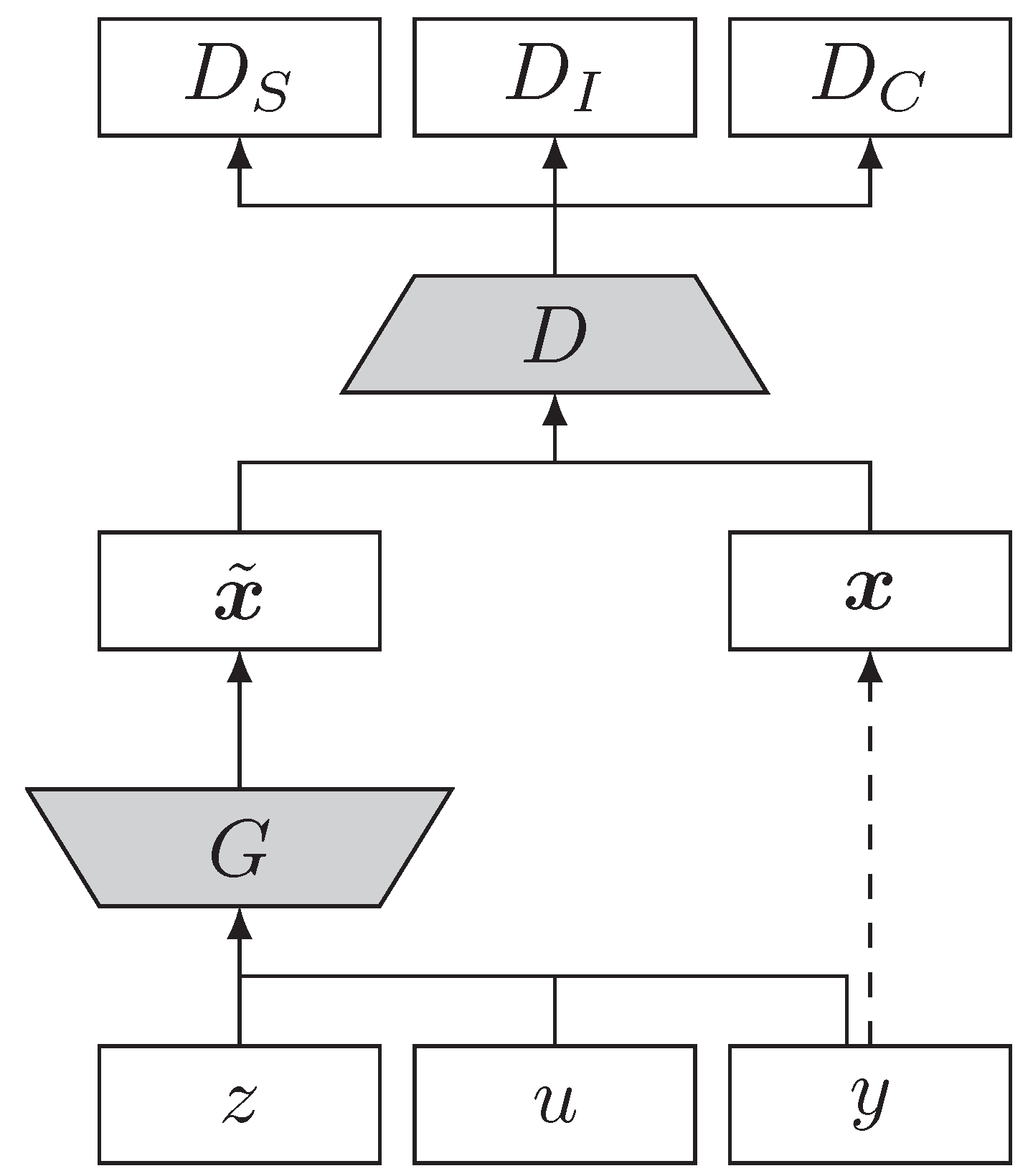
The configuration of WacGAN-info is visualized in Figure 1. The figure shows how G inputs three vectors: z, y, and u, representing random noise, class encoding, and latent info encoding, respectively. The output from G is an artificial data sample, $\tilde{\mathit{x}}$. Additionally, D inputs either real data samples, $\mathit{x}$, or artificial data samples, $\tilde{\mathit{x}}$. The output of D are three parallel signals: $D_S$, $D_C$, and $D_I$, which correspond to the estimation of the data source distribution (real or artificial samples), the class, and the latent info variable, respectively.

2.1. Objective Function

The objective function is divided into three parts: a source loss, $L_S$, a class loss, $L_C$, and an info loss, $L_I$.

The source loss, $L_S$, is responsible for distinguishing between the real and artificial data distributions given the discriminator output, $D_S$. $L_S$ is implemented as a Wasserstein loss with gradient penalty, which provides a high degree of diversity in the generated samples [16]. $L_S$ is given by

$$L_S=\underset{\mathit{x}\sim p_r}{\mathbb{E}}\left[D_S\left(\mathit{x}\right)\right]-\underset{\tilde{\mathit{x}}\sim p_g}{\mathbb{E}}\left[D_S\left(\tilde{\mathit{x}}\right)\right]+\lambda \underset{\widehat{\mathit{x}}\sim p_{\widehat{\mathit{x}}}}{\mathbb{E}}\left[{\left({\parallel {\nabla }_{\widehat{\mathit{x}}}{D}_S\left(\widehat{\mathit{x}}\right)\parallel }_{{}_2}-1\right)}^2\right],$$

(1)

where $p_r$ is the real data distribution and $p_g$ is the artificial data distribution implicitly defined by $\tilde{\mathit{x}}=G(z,\tilde{y},u),$ $z\sim p\left(z\right)$, [16]. $p_{\widehat{\mathit{x}}}$ is a random sample distribution generated from random interpolation between the real and artificial samples [16].

The class loss, $L_C$, is responsible for guiding the generator to produce samples, which are visually distinguishable for each separate class. $L_C$ is implemented as the cross-entropy loss between the one-hot encoded class label, y, and the output of the discriminator’s classification branch, $D_C\left(\mathit{x}\right)$ [4,23]. $L_C$ is given by:

$$L_C=\underset{\mathit{x}\sim p_r}{\mathbb{E}}\left[-\sum _{k\in N_C}{y}_{k}log{D}_{C_k}\left(\mathit{x}\right)\right]+\underset{\tilde{\mathit{x}}\sim p_g}{\mathbb{E}}\left[-\sum _{k\in N_C}{\tilde{y}}_{k}log{D}_{C_k}\left(\tilde{\mathit{x}}\right)\right],$$

(2)

where $N_C$ is the number of classes.

Finally, the info loss, $L_I$, ensures information preservation throughout the network, thus allowing the content of the generated samples to be controlled through a set of latent variables, u, as inspired by Chen et al. [4]. $L_I$ is implemented as the mean square loss between the intended info variables u and the predicted info variables of the discriminator $D_I\left(\mathit{x}\right)$ and is given by

$$L_I=\underset{\tilde{\mathit{x}}\sim p_g}{\mathbb{E}}\left[\sum _{i\in N_I}{(u_i-D_{I_i}\left(\tilde{\mathit{x}}\right))}^2\right],$$

(3)

where $N_I$ is the number of latent variables.

The discriminator is trained to minimize $-L_S+w_C{L}_C+w_I{L}_I$, whereas the generator is trained to minimize $L_S+w_C{L}_C+w_I{L}_I$. $w_C$ and $w_I$ are weight terms used to regulate the relative importance between the source loss, the class loss, and the info loss. The values of the $w_C$ and $w_I$ are determined empirically through experiments.

2.2. Network Design

The network architectures of the WacGAN-info model are inspired by the ACGAN model by [6]. As WacGAN-info is an extension of previous work [13], we apply the same modifications of the original ACGAN architecture. Additionally, the networks have been modified to accommodate for the additional information branch by adding a set of latent variables, u, as input to the generator and an additional output, $D_I$, to the discriminator to reproduce u. u are drawn from a random uniform distribution $p\left(u\right)\sim U(-1,1)$. u are concatenated with the categorical class encoding y and the noise vector z. The $D_I$ is implemented as a fully connected layer in parallel with the source discriminator, $D_S$, and the class discriminator, $D_C$, (Figure 1). The full implementation is summarized in Appendix A.1.

2.3. Evaluation

The artificial samples were evaluated qualitatively and quantitatively to assess their quality. In the qualitative evaluation, we performed a visual inspection of the artificial samples to provide a subjective assessment of the sample’s quality. The visual inspection was primarily used to assess the realism of the artificial samples (Does the sample look as a realistic plant?), as to our knowledge, there does not exist a quantitative metric to measure the realism of images.

In the quantitative evaluation, the class discriminability (How well does the artificial sample represent the intended species?) was evaluated by processing each sample using an external state-of-the-art classifier trained for plant species classification. Previously, the inception score [24] has been widely adopted as a metric for measuring the class discriminability in GAN research [5,6,16,21]. Madsen et al. [13] apply a similar approach where the external classifier is instead based on the ResNet-101 architecture [25], which is fine-tuned for plant seedling classification. To be able to directly compare the results, we applied the same external classifier as in [13]. The configuration of the external ResNet-101 classifier is summarized in Appendix A.2. The class discriminability is reported as the recognition accuracy, which indicates how often the artificial samples are correctly classified as the intended species by the external classifier [13]. Perfectly generated artificial samples will be indistinguishable from the real samples in terms of classification accuracy by the ResNet-101 classifier.

We applied the same leave-p-out cross validation scheme as Madsen et al. [13] to avoid data leakage in the quantitative results [26] and to be able to directly compare our results to Madsen et al. [13]. By splitting the real data into four parts and using a p of $50\%$, we get six combinations of training and test sets. For each combination, the external ResNet-101 classifier was trained on the associated training set and the WacGAN-info model was trained on the corresponding test set. Thus, the WacGAN-info model could be used to generate an additional test-set of artificial samples for the class discriminability test on the ResNet-101 classifier.

3. Results

Both the WacGAN-info model and the external ResNet-101 classifier were trained on the segmented plant seedling dataset (sPSD) by Giselsson et al. [27]. This dataset consists of segmented RBG images of plant seedlings from twelve different species. However, in this work, we have ignored all grass species as these are not properly instance segmented. This left nine species ($N_C=9$) remaining in the dataset. The plant species are identified by their European and Mediterranean Plant Protection Organization (EPPO) codes [28] throughput the paper. Due to the network’s architecture, the WacGAN-info model only supports input images with a resolution of $128\times 128$ pixels. To maintain a relatively low resizing factor, all images with a resolution of >400 pixels in either dimension are excluded from the dataset. This results in a resizing factor of $400/128=3.125$. The remaining species and number of samples for each of these are summarized in

Table 1. Overview of data in sPSD after removing grass species and images with a resolution larger than 400 pixels in either dimension.

Common Name	Latin Name	EPPO Code	N Samples
Charlock	Sinapis arvensis	SINAR	297
Cleavers	Galium aparine	GALAP	270
Common chickweed	Stellaria media	STEME	591
Fat hen	Chenopodium album	CHEAL	447
Maize	Zea mays	ZEAMX	149
Scentless mayweed	Matricaria perforata	MATIN	498
Shepherd’s purse	Capsella bursa-pastoris	CAPBP	225
Small-flowered cranesbill	Geranium pusillum	GERPU	429
Sugar beets	Beta vulgaris var. altissima	BEAVA	191

.

To train the WacGAN-info model, all of the images were preprocessed by: zero-padding to achieve a resolution of $470\times 470$ pixels, random rotation of the image, central crop of $400\times 400$ pixels, and finally, resizing to $128\times 128$ pixels using bilinear interpolation. This data augmentation approach is also used for training of the external ResNet-101 classifiers.

The regularization weights, $w_C$ and $w_I$, are set to $7.5$ and 15, respectively. As mentioned, these values are determined empirically and provide a good trade-off between intra- and inter-class diversity in the artificial samples, while allowing the latent variables to adapt dominating modalities in the data. The length of the noise vector, z, is set to 128, as inspired by previous work [13]. The following results are produced using two latent variables ($N_I=2$). A full summary of the hyperparameters can be found in Appendix A.1.

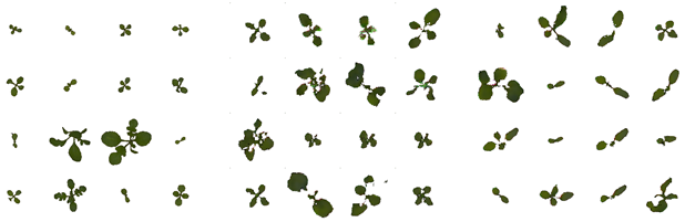
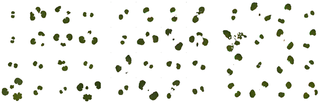
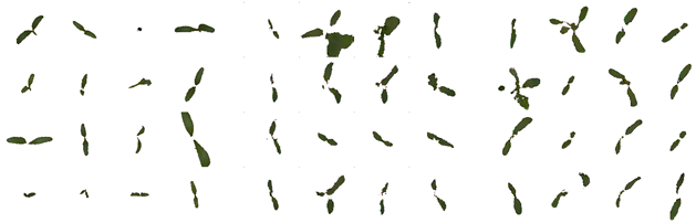
3.1. Visual Image Quality Assessment

Table 2. Examples of plant seedlings from sPSD [27], WacGAN [13], and WacGAN-info. The 16 samples for each species were generated using the same fixed random noise vectors, with only the class encoding changing. The background for all samples has been changed from black to white to increase the contrast.

	sPSD [27]	WacGAN [13]	WacGAN-Info (Ours)
SINAR
GALAP
STEME
CHEAL
ZEAMX
MATIN
CAPBP
GERPU
BEAVA

show examples of artificial plant seedlings generated using the WacGAN-info model. The table also includes examples of real plant seedlings and artificial samples from the WacGAN model to provide references for the visual evaluation. The 16 WacGAN-info samples for each species were generated using the same fixed random noise vectors—only the class encoding changes. This shows that the WacGAN-info model is capable of producing visually distinct samples for each of the different species present in the sPSD, as the appearance of the samples changes for each column.

The artificial samples themselves are composed of a number of leaves that are distributed around the image/plant center. Compared to the samples produced in Madsen et al. [13], the WacGAN-info model is capable of generating more detailed shape and textural features; e.g., the WacGAN-info model has become better at generating thin features such as stems or small leaves. The texture across a single leaf can also assume different gradients of green, whereas previously, the texture mainly consisted of a single green color. Additionally, the borders between the plant and background are more smooth for the WacGAN-info sample, whereas the WacGAN samples [13] are more rough around the edges.

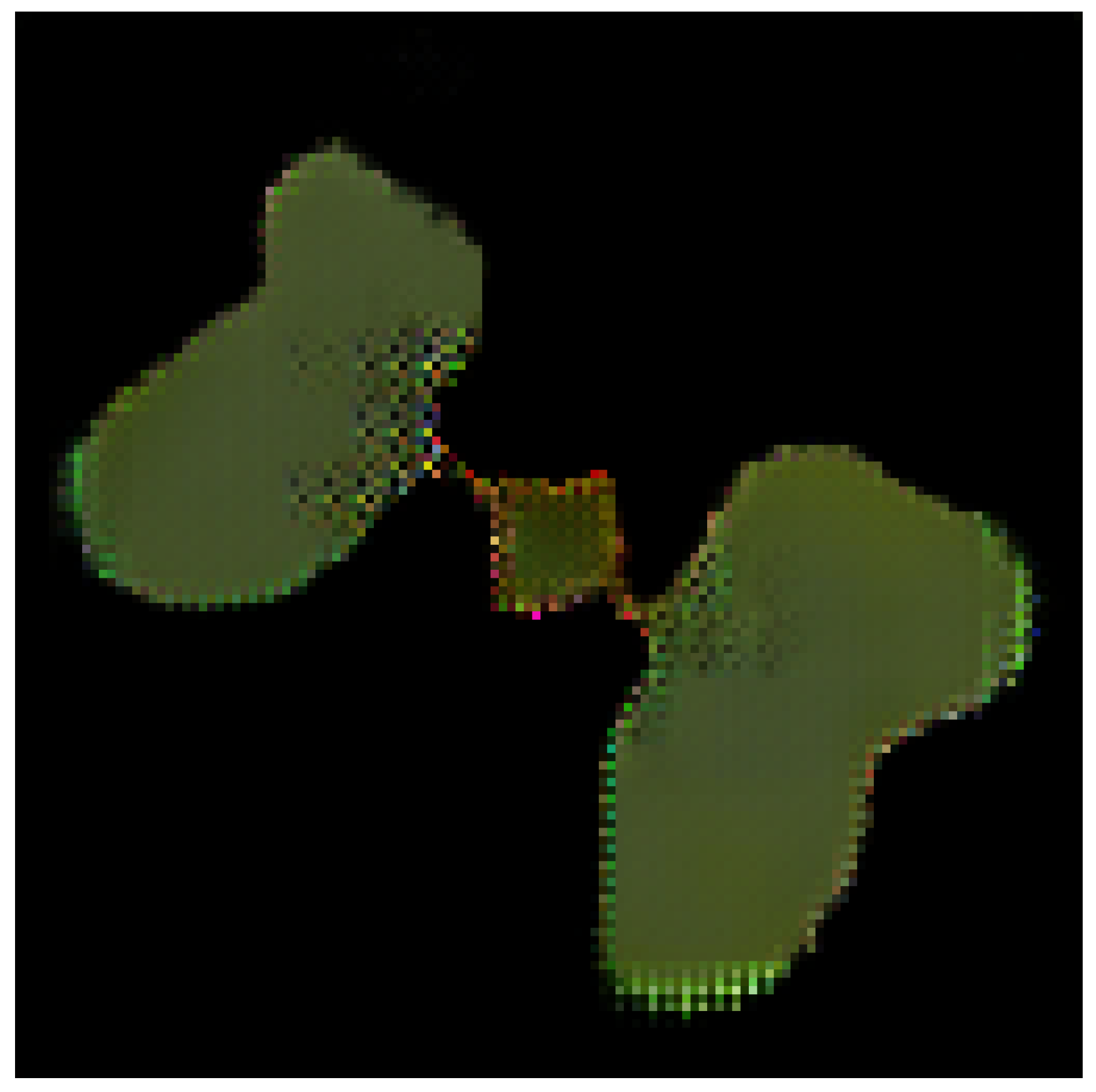
At closer inspection of the generated samples, some image artefacts can be observed. The artefacts can be described as pixel errors, which mainly occur along the border of the artificial samples or in a systematic grid in the texture. Figure 2 shows a severe example of these errors.

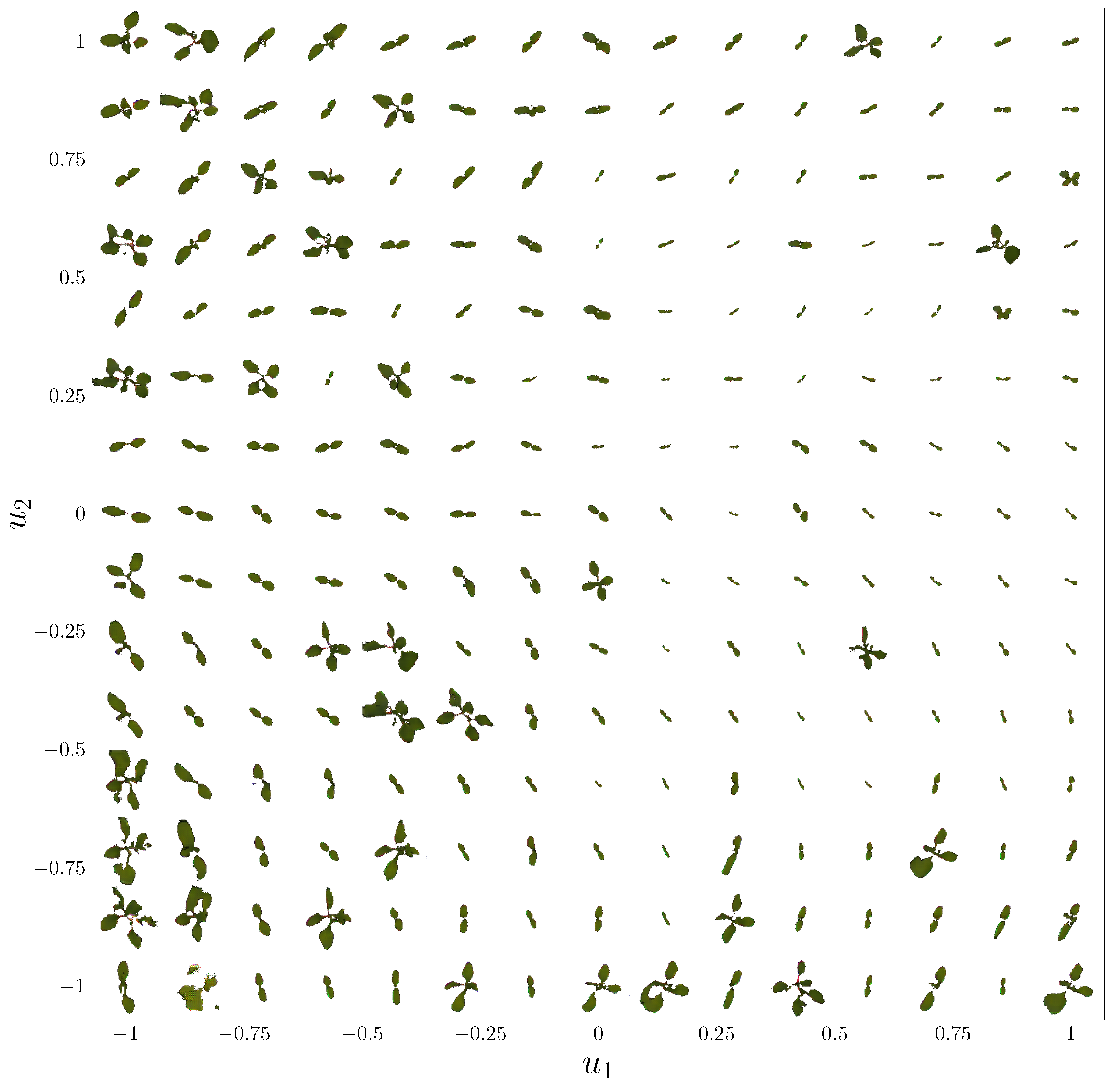
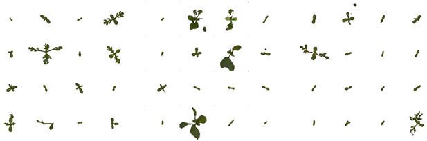
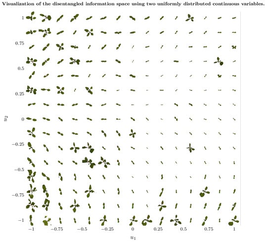
3.1.1. Disentangled Information Space

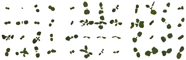
Figure 3 shows how the appearance of the artificial samples depends on the values of the two latent variables, $u_1$ and $u_2$. Although a few outliers are observed, the latent variables can, in this example, be used to control the rotation and the size of the artificial plant samples; e.g., the samples in the left-hand side of the plot are larger compared to those in the right-hand side, indicating that the size of the artificial samples is inversely related to the value of $u_1$. Additionally, the samples in the bottom of the plot are primarily oriented vertically with respect to the primary axis of the plant, whereas samples in the top are oriented horizontally, indicating that $u_2$ models the rotation of the samples.

Figure 3 only show the results from a single species, but a similar trend is observed across the other species as well. It should be noted that this specific trend is not unanimous across the six different models as they are trained on different parts of sPSD.

3.2. Class Discriminability

To assess the class discriminability of the artificial samples, 10,000 samples from each class ere generated from each of the six WacGAN-info generators and subsequently evaluated on the corresponding external ResNet101 classifiers along with the corresponding real data test sets (

Table 3. The accuracy of recognizing the intended species of the artificial samples from WacGAN-info, when analyzed using an external ResNet101 classifier trained solely on real data samples from sPSD. The recognition accuracies are reported as the mean and standard deviation over the six combinations in the cross-validation scheme.

Species	Test Set
	Real Data		Artificial Data
	N Samples	Accuracy	N Samples	Accuracy
SINAR	149	$94.3\pm 1.1\%$	10,000	$61.7\pm 21.8\%$
GALAP	135	$93.5\pm 2.3\%$	10,000	$63.6\pm 10.4\%$
STEME	296	$96.3\pm 0.7\%$	10,000	$89.0\pm 5.4\%$
CHEAL	224	$95.3\pm 1.7\%$	10,000	$63.4\pm 14.2\%$
ZEAMX	75	$90.5\pm 3.1\%$	10,000	$47.2\pm 16.6\%$
MATIN	249	$94.3\pm 1.6\%$	10,000	$67.0\pm 17.3\%$
CAPBP	113	$84.0\pm 3.1\%$	10,000	$47.4\pm 8.4\%$
GERPU	215	$95.8\pm 1.5\%$	10,000	$80.7\pm 6.5\%$
BEAVA	96	$90.6\pm 4.8\%$	10,000	$59.0\pm 12.0\%$
Total	1549	$92.7\pm 1.0\%$	90,000	$64.3\pm 4.4\%$

). The artificial data achieves $64.63\%$ average recognition accuracy when analyzed on the external classifiers. The average accuracy for recognizing real data samples is of course better compared to the artificial. However, the best-performing class on the artificial data (STEME) performs better than the worst-performing class on the real data (CAPBP). The average recognition accuracy for each class shows a strong positive linear correlation to the number of real samples for each class in both the real data ($\rho =0.70$) and the artificial data ($\rho =0.85$).

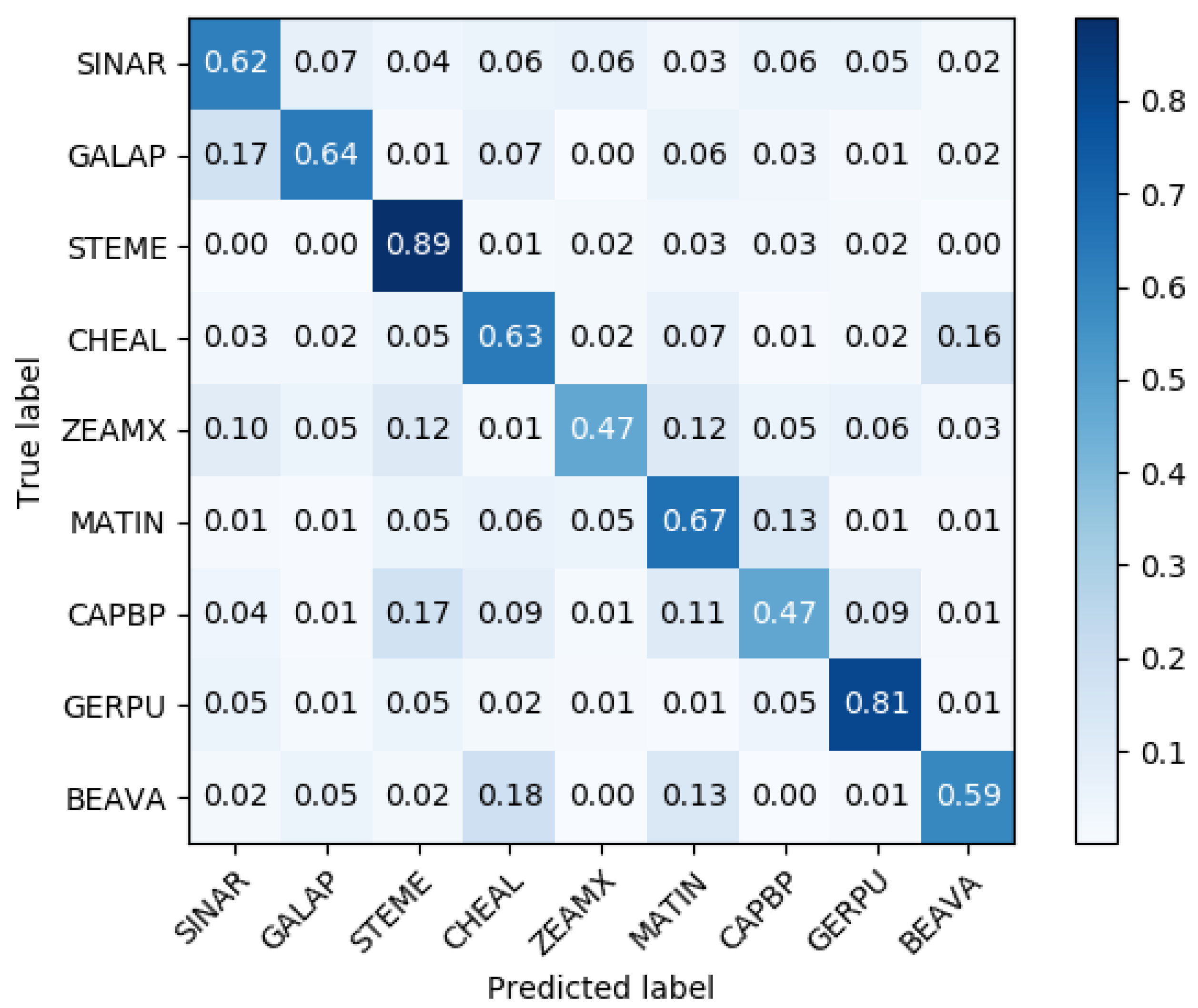
From the confusion matrix (Figure 4), it is clear that there is a good correspondence between the true labels and the predicted labels on the artificially generated data. The misclassifications (the off-diagonal entries in the confusion matrix) are generally fairly uniformly distributed among the other species; however, a few notable misclassifications do appear, which are significantly larger than the other misclassifications. These can be grouped into two groups: (1) one-way misclassifications and (2) two-way misclassifications. The two-way misclassifications are misclassifications between two species, which are both significantly larger than the other misclassifications (CHEAL ⇄ BEAVA, and MATIN ⇄ CAPBP). The misclassifications between CHEAL and BEAVA occur in samples mimicking the early growth stages, where both species are highly similar with respect to visual appearance. A large portion of the mislcassifications from BEAVA to CHEAL also includes examples of large broad leafs mixed with more elongated leafs, traits that occur in the real examples of CHEAL but not BEAVA. In the one-way misclassifications, there is only a significant misclassification from one species to the other, but not the other way around (CAPBP → {STEME, GERPU, CHEAL}, ZEAMX → {STEME, MATIN, SINAR}, GALAP → SINAR, and BEAVA → MATIN). These misclassifications generally happen from species with relatively few samples to species with relatively many classes in the real dataset. A notable exception to this is the misclassification of GALAP as SINAR, which contain approximately the same number of samples in the real dataset. These misclassifications consists of two medium-sized round leafs connected by a small stem. Although the GALAP real data does contain samples with these leafs, the trait occurs much more frequently in the SINAR real data.

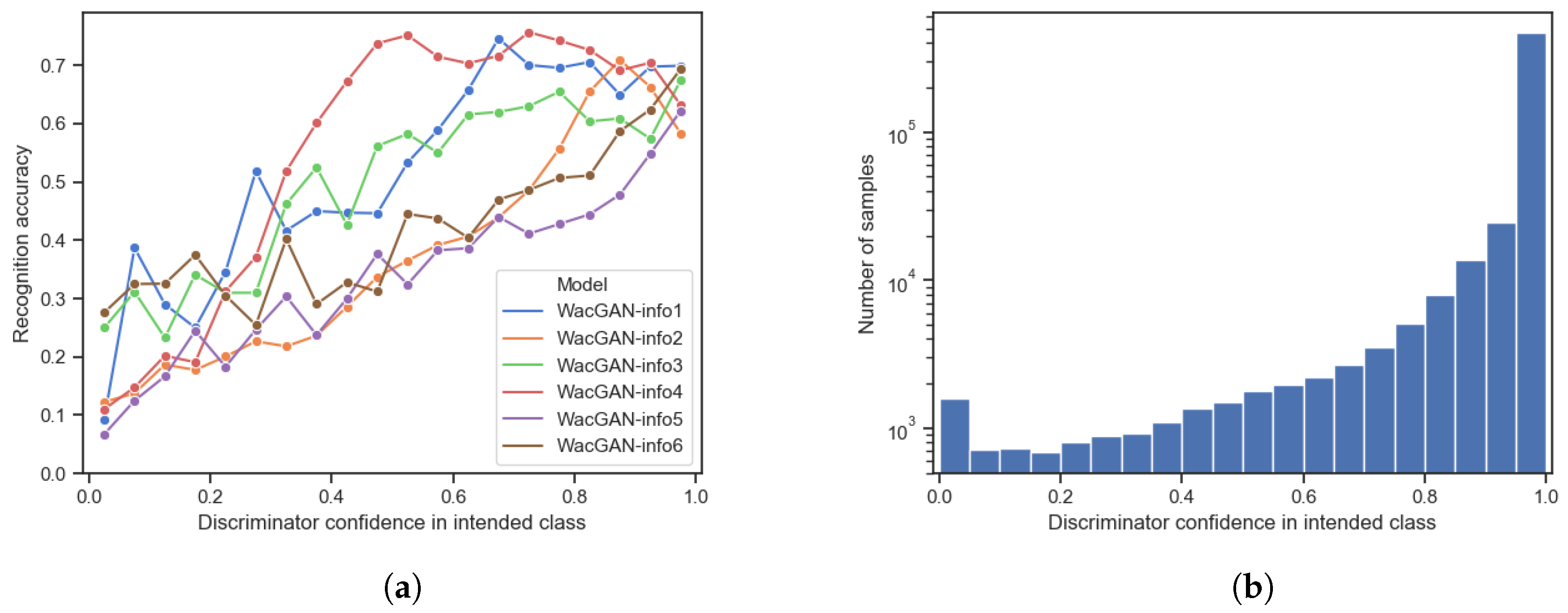
Using the GAN Descriminator to Prevalidate Sample Quality

The recognition accuracies reported in Table 3 are based on all samples generated by the WacGAN-info model. However, the classification branch of the discriminator, $D_C\left(x\right)$, can be used to perform a prevalidation of the artificial samples. Due to the softmax activation, $D_C\left(x\right)$ outputs a confidence of how well a sample represents each class. Thus, by examining the discriminator’s confidence in the intended class for each artificial sample, we can assure better class representations. Figure 5 shows the average recognition accuracy (Figure 5a) and the sample distribution (Figure 5b) as a function of the discriminator’s confidence in the samples representing the intended class. The figure shows that the artificial samples generally get recognized as the intended class more often by the external classifier, if the discriminator also has high confidence in the samples belonging to the intended class. Thus, it is possible to remove samples with poor class representations by applying a threshold on the discriminator’s confidence in each sample. Additionally, Figure 5b shows that the WacGAN-info discriminator has high confidence in the majority of the artificial samples, so if we threshold on the discriminator confidence, we only remove a small part of the data; e.g., by including only samples with a discriminator confidence greater than $0.95$, the average recognition accuracy across the six models increases from $64.3\%$ to $65.3\%$, while still including the $86\%$ of the artificial samples.

4. Discussion

The results show that the WacGAN-info model is capable of producing artificial samples that resemble real plant seedlings. Furthermore, it seems that the model is capable of reproducing samples that are relatively distinguishable across the nine different plant species while simultaneously ensuring a relatively high degree of variability in the samples for each class.

Although the WacGAN-info samples visually resemble real plant seedlings, there are still some obvious errors in the artificial samples. The errors are mainly related to unrealistic or inaccurate reproductions of the plant leaves, where multiple leaves have merged into one or one has been split into two or more; e.g., inspecting the samples of ZEAMX, some of these resemble dicots although ZEAMX is a monocot species (see the first and last samples in Table 2). These visual errors may be reduced by increasing the class loss weight, $w_C$, which seems to provide better inter-class diversity but comes at the cost of reducing the intra-class diversity.

The observed pixel errors in the samples are probably related to the applied generator architecture as the border errors could be related to the relatively large output kernel ($[8\times 8]$) and the grid pattern matches with strides of 2 used for the up-sampling. Similar errors were observed in the original ACGAN [6] paper and in the previous work by Madsen et al. [13]; however, based on visual inspection, the issue seems to have been reduced for the WacGAN-info model.

Section 3.1.1 shows that it is possible to control the appearance of the generated samples through the latent information variables. As expected, the information variables capture dominating modalities in the data, such as the size and rotation of the samples. Although the two latent variables control similar properties in all six WacGAN-info models, it should be noted that the specific trend observed in Figure 3 is not representative of all models. This is an effect of the models being trained on different dataset splits and due to the unsupervised learning scheme applied in the information learning branch, which causes the models to adopt slightly different trends. In this work, we only present results using two uniformly distributed information variables ($N_I=2$); the setup can easily be extended to facilitate more, but adding more latent variables quickly increases the complexity of interpreting their underlying representation.

The class discriminability test (Section 3.2) also shows that the artificial samples resemble the intended species to a relatively high degree. The reported average recognition accuracy is $64.3\%$ (see Table 3), which is well above uniformly distributed random guessing, which would yield $11.1\%$. Compared to Madsen et al. [13], this result shows a 5.4% point increase in the overall recognition accuracy and a 4.4% point decrease in the standard deviation thereof. As this work is an extension of Madsen et al. [13], the GAN setup is relatively similar. tThe main difference is that the WacGAN-info model includes the additional latent information variables u and information discriminator $D_I\left(\mathit{x}\right)$. This shows that the addition of the latent information variables not only helps control the appearance of the generated samples but also helps to increase the discriminability of the species.

The observed errors in the class discriminability test appear to mainly stem from class imbalance in the real training data, as artificial samples from species with more training samples generally achieve higher recognition accuracies. This issue might be reduced by balancing the distribution between the classes in the training. Additionally, the observed errors are also related to species, which are visually similar at the early growth stages. This is probably a result of the models incapability of reproducing small textural and shape details. Through visual inspection of the errors, it is also observed that some samples include attributes that are not present in the “true” species, but only in the “misclassified” samples. This shows attribute leakage between the species examples produced by the generator and that the generator has not fully learned what constitutes each species and what separates them. This leakage mainly occurs in the generated samples of larger plants. Many plant species develop their visual characteristics as they grow larger. However, in this work, we have removed many of the larger samples (>400 pixels in either dimension) to maintain a relatively small resizing factor in the preprocessing of the images. By including these larger images in the training, it might be possible to learn more about the individual species characteristics and avoid some of the above-mentioned errors. However, to include these larger images, we would need larger network architectures for the generator and the discriminator, which would make the training more unstable [6]. A potential solution could be to apply a more advanced conditioning scheme [21,22] or a progressive growing GAN training approach [29].

Section 3.2 showed that it is possible to remove samples with poor class representation from the artificial data distribution by evaluating the discriminator’s confidence in each artificial sample. This enables us to only select samples that have a relatively higher resemblance to real plant seedlings, which is relevant if the samples are used for data augmentation purposes or in transfer learning, as previously shown in [13]. However, the selection process may remove some variability from the artificial samples, but probably not anything too severe since $86\%$ of the samples remain even with a $D_C$ confidence threshold of >0.95.

5. Conclusions

In this paper, we have shown that the WacGAN-info model is capable of producing artificial samples from nine different species. The artificial samples resemble the intended species with an average recognition accuracy of $64.3\%$ evaluated using an external state-of-the-art classification model, which is an improvement of $5.4\%$ points compared to previous work. The observed errors are mostly related to class imbalances in the training data or to the applied network models, which are incapable pf reproducing small textural and shape details in the samples. We have also shown that it is possible to apply an unsupervised conditioning scheme in the training of WacGAN-info, which enables control over the visual appearance of the samples through a set of latent variables. Specifically, we show that it is possible to control the orientation and size of the samples through two latent variables. Finally, we have shown that it is possible to apply the discriminator as a quality assessment tool, which can be used to remove samples with poor class representation from the artificial data distribution, further increasing the recognition accuracy to $65.3\%$.