Comparing DInSAR and PSI Techniques Employed to Sentinel-1 Data to Monitor Highway Stability: A Case Study of a Massive Dobkovičky Landslide, Czech Republic


Abstract

1. Introduction
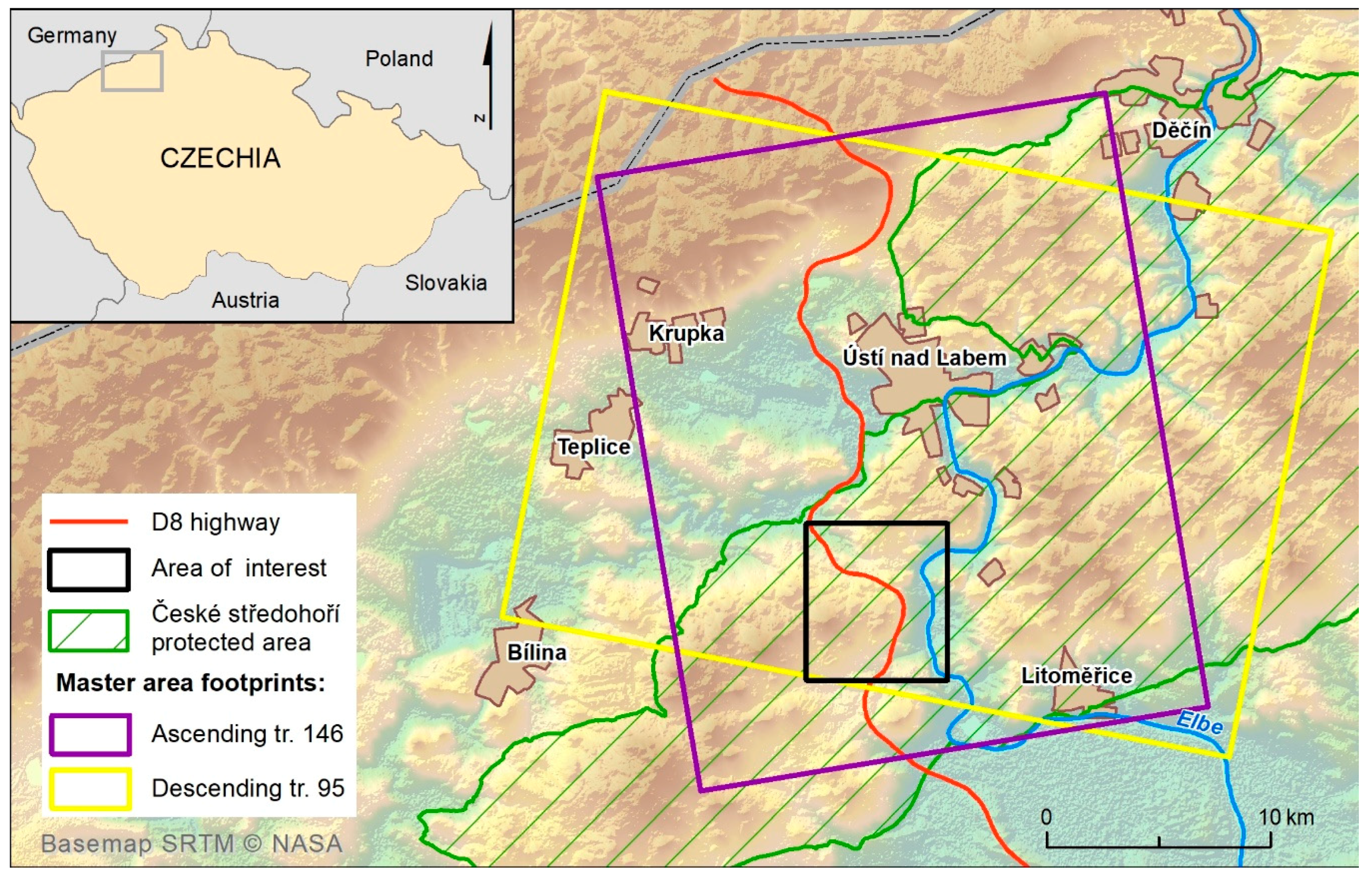
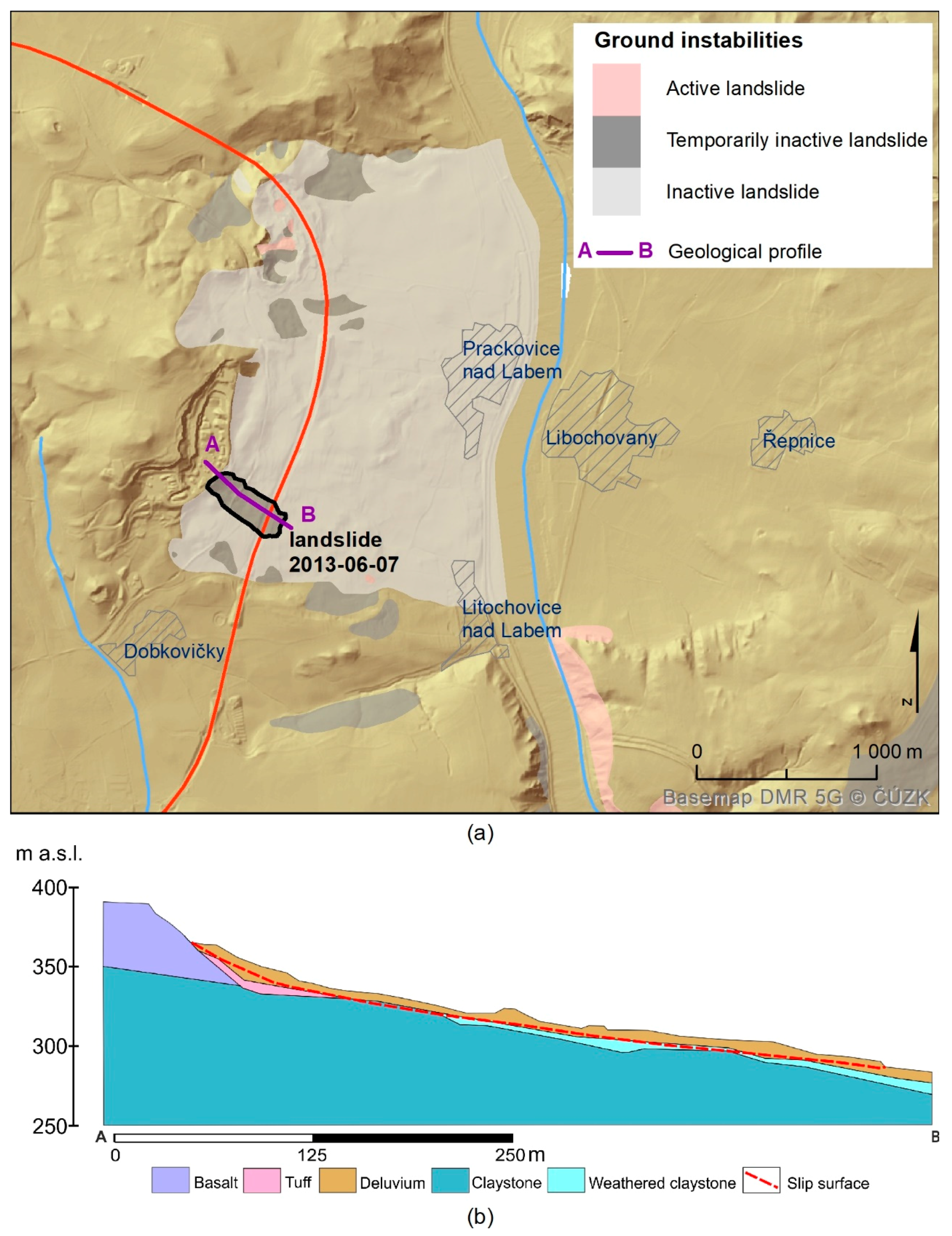
2. Study Area
3. Dataset Description
4. Methodology
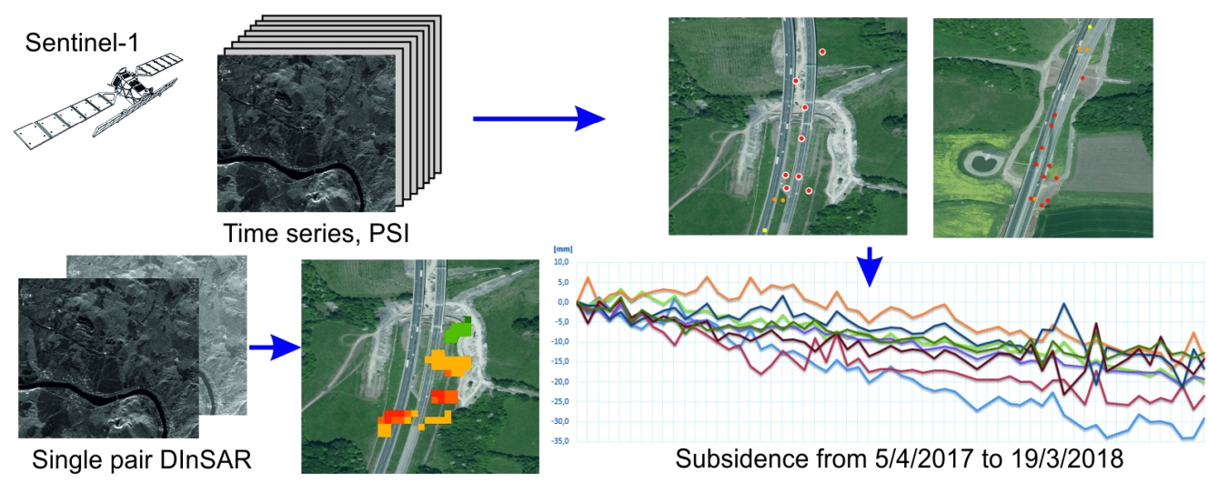
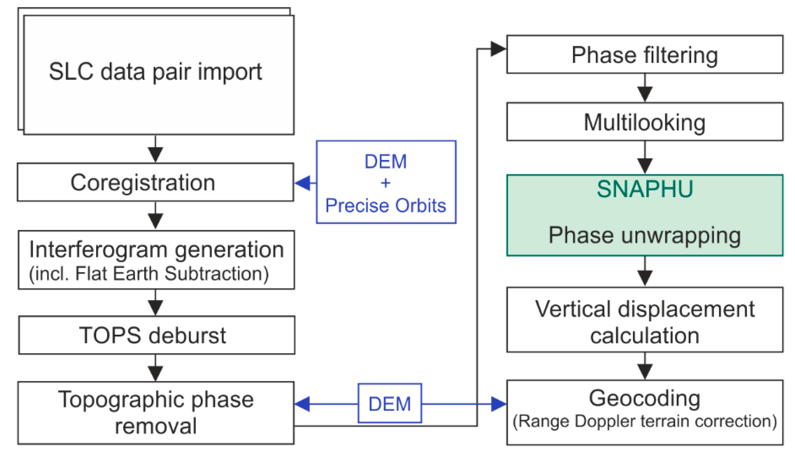
4.1. Scenario 1: The Single Pair DInSAR
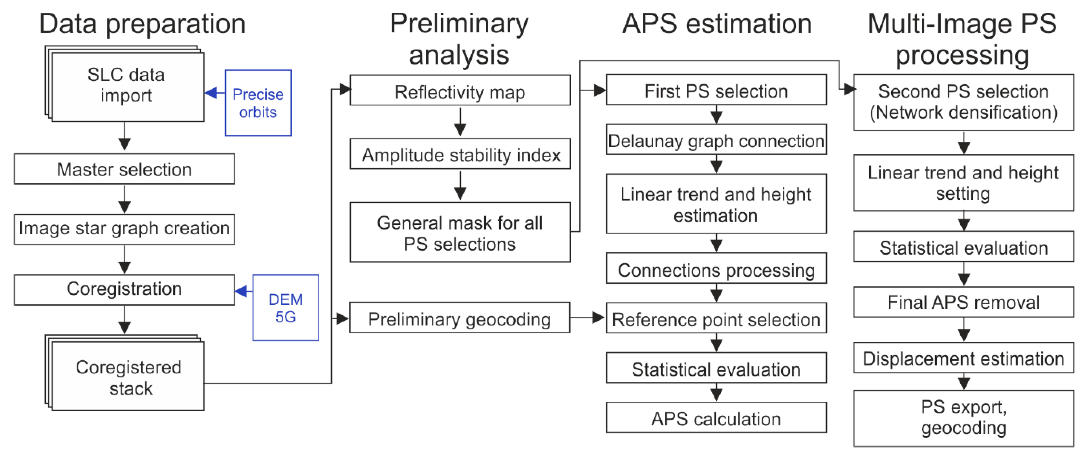
4.2. Scenario 2: The PSI
- It must be acquired under good weather conditions (no rain); and
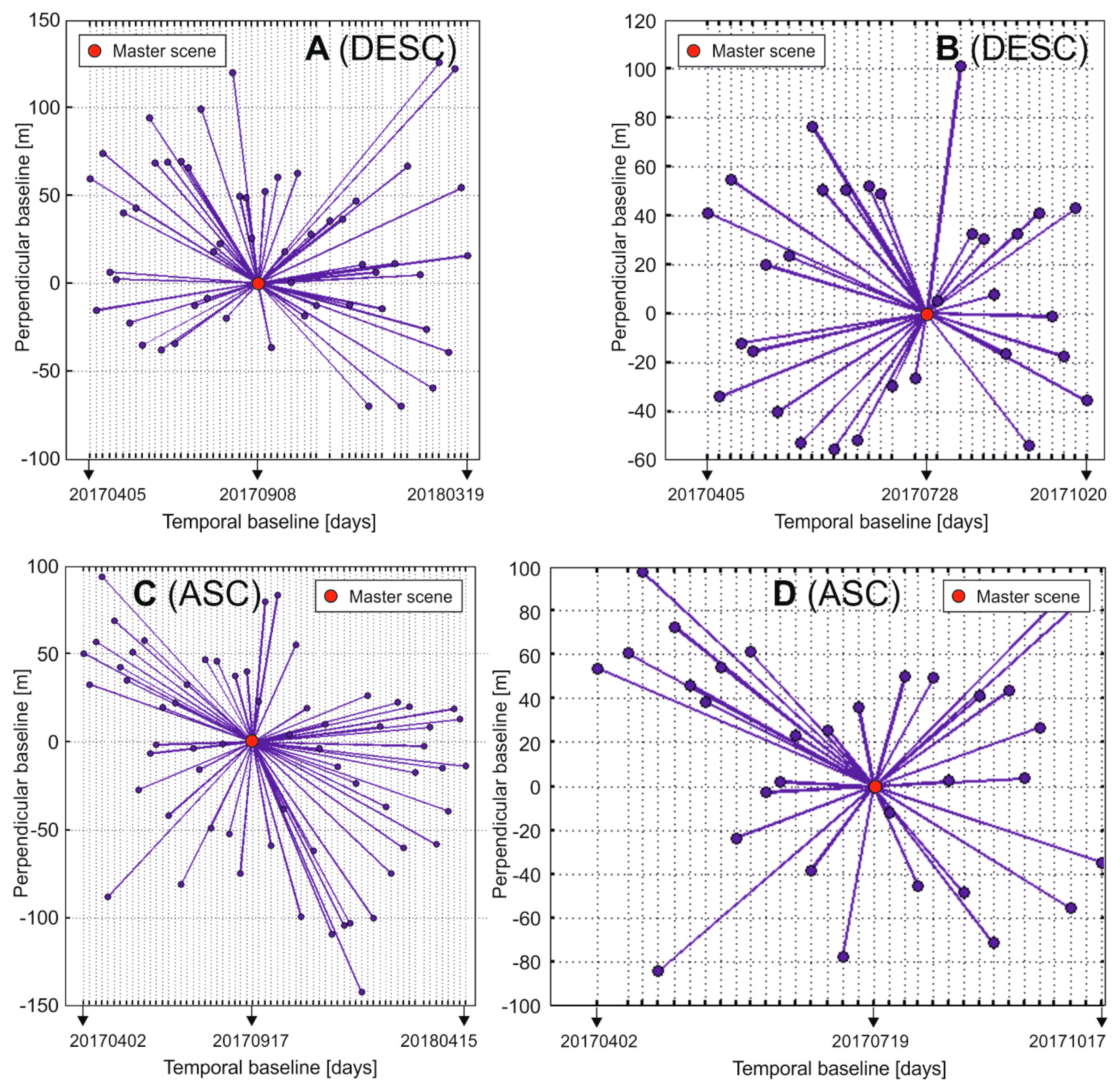
- It has a suitable position (approximately in the middle) in the image star graph considering the perpendicular and temporal baseline [54].
5. Results
5.1. Scenario 1: Single Pair DInSAR Results
5.2. Scenario 2: The PSI Results
6. Validation
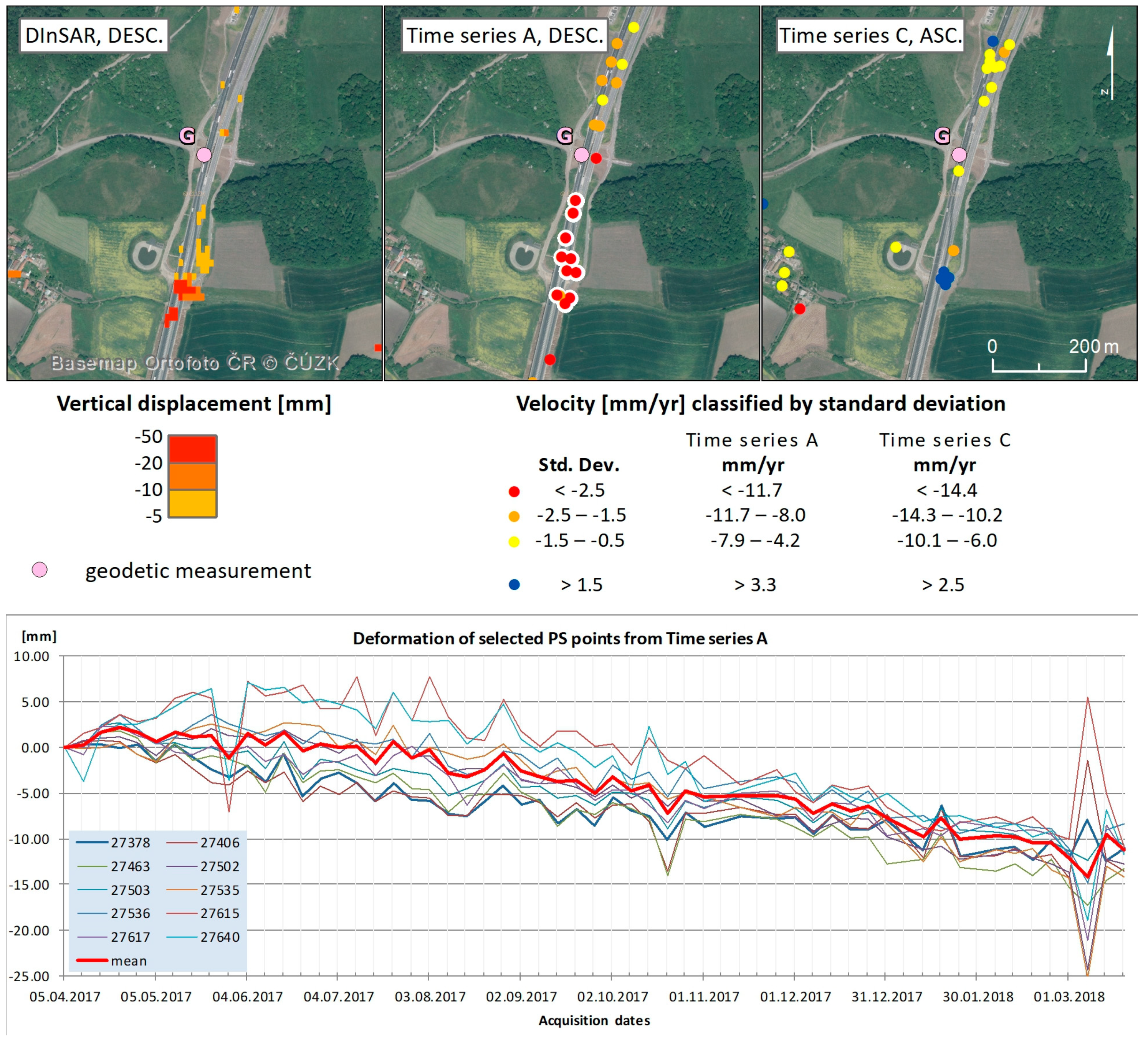
6.1. Area 1: Highway Embankment Between Ječky Bridge and Dobkovičky Bridge at km 55.700–56.000
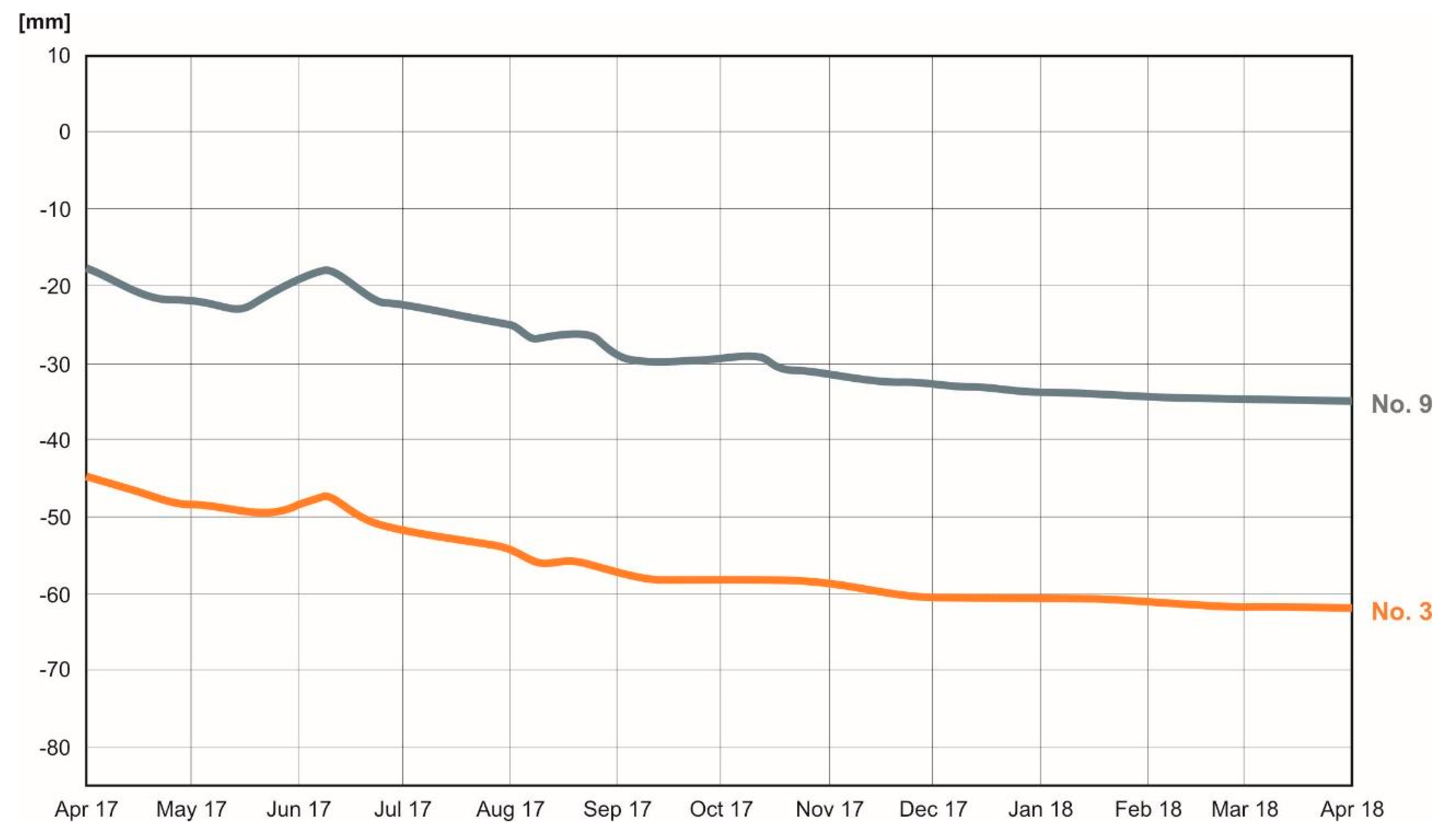
6.2. Area 2: Prackovice Bridge, 57,300–57,500 km
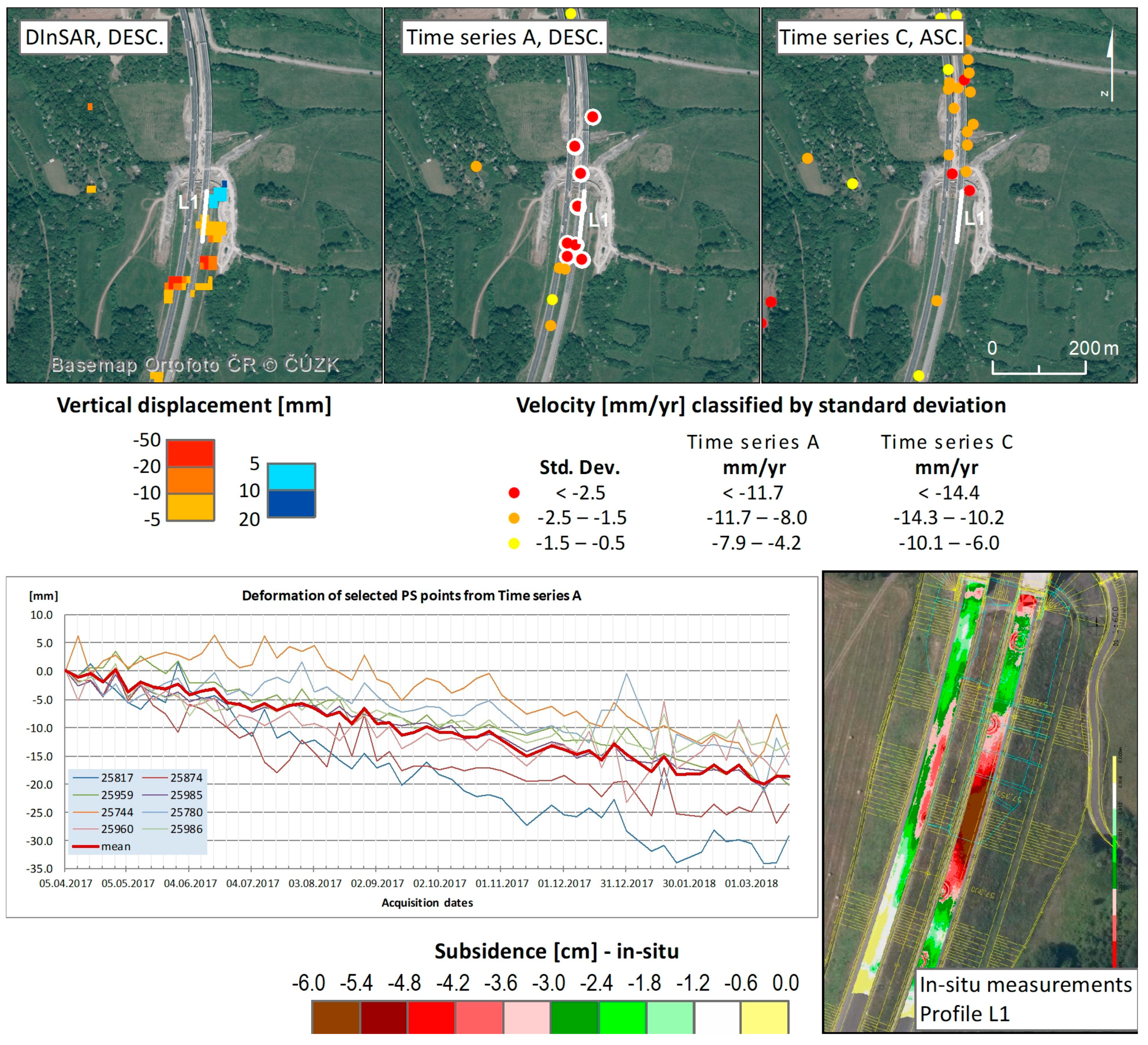
6.3. Area 3: Part between Two Highway Tunnels (“Prackovice” and “Radejčín”) at km 58,400
6.4. Area 4: Vertical Changes in the Dobkovičky Quarry
7. Discussion
8. Conclusions
Author Contributions
Funding
Acknowledgments
Conflicts of Interest
References
- Chae, B.G.; Park, H.J.; Catani, F.; Simoni, A.; Berti, M. Landslide prediction, monitoring and early warning: A concise review of state-of-the-art. Geosci. J. 2017, 21, 1033–1070. [Google Scholar] [CrossRef]
- Béjar-Pizarro, M.; Notti, D.; Mateos, R.M.; Ezquerro, P.; Centolanza, G.; Herrera, G.; Bru, G.; Sanabria, M.; Solari, L.; Duro, J.; et al. Mapping Vulnerable Urban Areas Affected by Slow-Moving Landslides Using Sentinel-1 InSAR Data. Remote Sens. 2017, 9, 876. [Google Scholar] [CrossRef]
- Stumpf, A.; Malet, J.P.; Delacourt, C. Correlation of satellite image time-series for the detection and monitoring of slow-moving landslides. Remote Sens. Environ. 2017, 189, 40–55. [Google Scholar] [CrossRef]
- Raspini, F.; Ciampalini, A.; Del Conte, S.; Lombardi, L.; Nocentini, M.; Gigli, G.; Ferretti, A.; Casagli, N. Exploitation of Amplitude and Phase of Satellite SAR Images for Landslide Mapping: The Case of Montescaglioso (South Italy). Remote Sens. 2015, 7, 14576–14596. [Google Scholar] [CrossRef]
- Singleton, A.; Li, Z.; Hoey, T.; Muller, J.-P. Evaluating sub-pixel offset techniques as an alternative to D-InSAR for monitoring episodic landslide movements in vegetated terrain. Remote Sens. Environ. 2014, 147, 133–144. [Google Scholar] [CrossRef]
- Scaioni, M.; Longoni, L.; Melillo, V.; Papini, M. Remote Sensing for Landslide Investigations: An Overview of Recent Achievements and Perspectives. Remote Sens. 2014, 6, 9600–9652. [Google Scholar] [CrossRef]
- Casagli, N.; Cigna, F.; Bianchini, S.; Hölbling, D.; Füreder, P.; Righini, G.; Del Conte, S.; Friedl, B.; Schneiderbauer, S.; Iasio, C.; et al. Landslide mapping and monitoring by using radar and optical remote sensing: Examples from the EC-FP7 project SAFER. Remote Sens. Appl. Soc. Environ. 2016, 4, 92–108. [Google Scholar] [CrossRef]
- Gabriel, A.K.; Goldstein, R.M.; Zebker, H.A. Mapping small elevation changes over large areas: Differential radar interferometry. J. Geophys. Res. 1989, 94, 9183–9191. [Google Scholar] [CrossRef]
- Raspini, F.; Bardi, F.; Bianchini, S.; Ciampalini, A.; Del Ventisette, C.; Farina, P.; Ferrigno, F.; Solari, L.; Casagli, N. The contribution of satellite SAR-derived displacement measurements in landslide risk management practices. Nat. Hazards 2017, 86, 327–351. [Google Scholar] [CrossRef]
- Przyłucka, M.; Herrera, G.; Graniczny, M.; Colombo, D.; Béjar-Pizarro, M. Combination of Conventional and Advanced DInSAR to Monitor Very Fast Mining Subsidence with TerraSAR-X Data: Bytom City (Poland). Remote Sens. 2015, 7, 5300–5328. [Google Scholar] [CrossRef]
- Zhao, C.; Lu, Z.; Zhang, Q.; De, J. Large-area landslide detection and monitoring with ALOS / PALSAR imagery data over Northern California and Southern Oregon, USA. Remote Sens. Environ. 2012, 124, 348–359. [Google Scholar] [CrossRef]
- Costantini, M.; Iodice, A.; Magnapane, L.; Pietranera, L. Monitoring terrain movements by means of sparse SAR differential interferometric measurements. In Proceedings of the 20th IEEE International Geoscience and Remote Sensing Symposium (IGARSS), Honolulu, HI, USA, 24–28 July 2000; pp. 3225–3227. [Google Scholar]
- Strozzi, T.; Farina, P.; Corsini, A.; Ambrosi, C.; Thüring, M.; Zilger, J.; Wiesmann, A.; Wegmüller, U.; Werner, C. Survey and monitoring of landslide displacements by means of L-band satellite SAR interferometry. Landslides 2005, 2, 193–201. [Google Scholar] [CrossRef]
- Catani, F.; Farina, P.; Moretti, S.; Nico, G.; Strozzi, T. On the application of SAR interferometry to geomorphological studies: Estimation of landform attributes and mass movements. Geomorphology 2005, 66, 119–131. [Google Scholar] [CrossRef]
- Calabro, M.D.; Schmidt, D.A.; Roering, J.J. An examination of seasonal deformation at the Portuguese Bend landslide, southern California, using radar interferometry. J. Geophys. Res. 2010, 115, F02020. [Google Scholar] [CrossRef]
- Barra, A.; Monserrat, O.; Mazzanti, P.; Esposito, C.; Crosetto, M.; Mugnozza, G.S. First insights on the potential of Sentinel-1 for landslides detection. Geomat. Nat. Hazards Risk 2016, 7, 1874–1883. [Google Scholar] [CrossRef]
- Wasowski, J.; Bovenga, F. Investigating landslides and unstable slopes with satellite multitemporal interferometry: Current issues and future perspectives. Eng. Geol. 2014, 174, 103–138. [Google Scholar] [CrossRef]
- Schlögel, R.; Thiebes, B.; Mulas, M.; Cuozzo, G.; Notarnicola, C.; Schneiderbauer, S.; Crespi, M.; Mazzoni, A.; Mair, V.; Corsini, A. Multi-Temporal X-Band Radar Interferometry Using Corner Reflectors: Application and Validation at the Corvara Landslide (Dolomites, Italy). Remote Sens. 2017, 9, 739. [Google Scholar] [CrossRef]
- Ferretti, A.; Prati, C.; Rocca, F. Permanent scatterers in SAR interferometry. IEEE Trans. Geosci. Remote Sens. 2001, 39, 8–20. [Google Scholar] [CrossRef]
- Berardino, P.; Fornaro, G.; Lanari, R.; Sansosti, E. A new algorithm for surface deformation monitoring based on small baseline differential SAR interferograms. IEEE Trans. Geosci. Remote Sens. 2002, 40, 2375–2383. [Google Scholar] [CrossRef]
- Mora, O.; Mallorqui, J.J.; Broquetas, A. Linear and Nonlinear Terrain Deformation Maps from a Reduced Set of Interferometric SAR Images. IEEE Trans. Geosci. Remote Sens. 2003, 41, 2243–2253. [Google Scholar] [CrossRef]
- Hooper, A.; Zebker, H.; Segall, P.; Kampes, B. A New Method for Measuring Deformation on Volcanoes and Other Natural Terrains Using Insar Persistent Scatterers. Geophys. Res. Lett. 2004, 31, 1–5. [Google Scholar] [CrossRef]
- Hooper, A.; Segall, P.; Zebker, H. Persistent Scatterer InSAR for Crustal Deformation Analysis, with Application to Volcán Alcedo, Galapagos. J. Geophys. Res. Solid Earth 2007, 112, 1–19. [Google Scholar] [CrossRef]
- Crosetto, M.; Biescas, E.; Duro, J.; Closa, J.; Arnaud, A. Generation of Advanced ERS and Envisat Interferometric SAR Products Using the Stable Point Network Technique. Photogramm. Eng. Remote Sens. 2008, 74, 443–451. [Google Scholar] [CrossRef]
- Perissin, D.; Wang, T. Repeat-pass SAR Interferometry with Partially Coherent Targets. IEEE Trans. Geosci. Remote Sens. 2012, 50, 271–280. [Google Scholar] [CrossRef]
- Lanari, R.; Lundgren, P.; Manzo, M.; Casu, F. Satellite radar interferometry time series analysis of surface deformation for Los Angeles, California. Geophys. Res. Lett. 2004, 31, L23–L613. [Google Scholar] [CrossRef]
- Guzzetti, F.; Manunta, M.; Ardizzone, F.; Pepe, A.; Cardinali, M.; Zeni, G.; Reichenbach, P.; Lanari, R. Analysis of Ground Deformation Detected Using the SBAS-DInSAR Technique in Umbria, Central Italy. Pure Appl. Geophys. 2009, 166, 1425–1459. [Google Scholar] [CrossRef]
- Herrera, G.; Gutiérrez, F.; García-Davalillo, J.C.; Guerrero, J.; Notti, D.; Galve, J.P.; Fernández-Merodo, J.A.; Cooksley, G. Multi-sensor advanced DInSAR monitoring of very slow landslides: the Tena Valley case study (Central Spanish Pyrenees). Remote Sens. Environ. 2013, 128, 31–43. [Google Scholar] [CrossRef]
- Calò, F.; Ardizzone, F.; Castaldo, R.; Lollino, P.; Tizzani, P.; Guzzetti, F.; Lanari, R.; Angeli, M.-C.; Pontoni, F.; Manunta, M. Enhanced landslide investigations through advanced DInSAR techniques: The Ivancich case study, Assisi, Italy. Remote Sens. Environ. 2014, 142, 69–82. [Google Scholar] [CrossRef]
- Dai, K.; Li, Z.; Tomás, R.; Liu, G.; Yu, B.; Wang, X.; Cheng, H.; Chen, J.; Stockamp, J. Monitoring activity at the Daguangbao mega-landslide (China) using Sentinel-1 TOPS time series interferometry. Remote Sens. Environ. 2016, 186, 501–513. [Google Scholar] [CrossRef]
- Crosetto, M.; Monserrat, O.; Devanthery, N.; Cuevas-Gonzalez, M.; Barra, A.; Crippa, B. Persistent Scatterer Interferometry Using Sentinel-1 Data. In Proceedings of the XXIII ISPRS Congress International Archives of the Photogrammetry, Remote Sensing and Spatial Information Sciences, Prague, Czech Republic, 12–19 July 2016; Volume XLI-B7. [Google Scholar] [CrossRef]
- Canuti, P.; Casagli, N.; Ermini, L.; Fanti, R.; Farina, P. Landslide activity as a geoindicator in Italy: Significance and new perspectives from remote sensing. Environ Geol. 2004, 45, 907–919. [Google Scholar] [CrossRef]
- Colesanti, C.; Wasowski, J. Investigating landslides with space-borne Synthetic Aperture Radar (SAR) interferometry. Eng. Geol. 2006, 88, 173–199. [Google Scholar] [CrossRef]
- Bovenga, F.; Wasowski, J.; Nitti, D.O.; Nutricato, R.; Chiaradia, M.T. Using COSMO/SkyMed X-band and ENVISAT C-band SAR interferometry for landslides analysis. Remote Sens. Environ. 2012, 119, 272–285. [Google Scholar] [CrossRef]
- Tofani, V.; Raspini, F.; Catani, F.; Casagli, N. Persistent Scatterer Interferometry (PSI) Technique for Landslide Characterization and Monitoring. Remote Sens. 2013, 5, 1045–1065. [Google Scholar] [CrossRef]
- Del Ventisette, C.; Righini, G.; Moretti, S.; Casagli, N. Multitemporal landslides inventory map updating using spaceborne SAR analysis. Int. J. Appl. Earth Obs. Geoinf. 2014, 30, 238–246. [Google Scholar] [CrossRef]
- Crosetto, M.; Monserrat, O. Persistent scatterer interferometry: Potentials and limits. In Proceedings of the ISPRS Hannover Workshop: High-Resolution Earth Imaging for Geospatial Information, Hannover, Germany, 2–5 June 2009. [Google Scholar]
- Czikhardt, R.; Papco, J.; Bakon, M.; Liscak, P.; Ondrejka, P.; Zlocha, M. Ground Stability Monitoring of Undermined and Landslide Prone Areas by Means of Sentinel-1 Multi-Temporal InSAR, Case Study from Slovakia. Geosciences 2017, 7, 87. [Google Scholar] [CrossRef]
- Barra, A.; Solari, L.; Béjar-Pizarro, M.; Monserrat, O.; Bianchini, S.; Herrera, G.; Crosetto, M.; Sarro, R.; González-Alonso, E.; Mateos, R.M.; et al. A Methodology to Detect and Update Active Deformation Areas Based on Sentinel-1 SAR Images. Remote Sens. 2017, 9, 1002. [Google Scholar] [CrossRef]
- Del Soldato, M.; Farolfi, G.; Rosi, A.; Raspini, F.; Casagli, N. Subsidence Evolution of the Firenze–Prato–Pistoia Plain (Central Italy) Combining PSI and GNSS Data. Remote Sens. 2018, 10, 1146. [Google Scholar] [CrossRef]
- Strozzi, T.; Klimeš, J.; Frey, H.; Caduff, R.; Huggel, C.; Wegmüller, U.; Rapre, A.C. Satellite SAR interferometry for the improved assessment of the state of activity of landslides: A case study from the Cordilleras of Peru. Remote Sens. Environ. 2018, 217, 111–125. [Google Scholar] [CrossRef]
- Raspini, F.; Bianchini, S.; Ciampalini, A.; Del Soldato, M.; Solari, L.; Novali, F.; Del Conte, S.; Rucci, A.; Ferretti, A.; Casagli, N. Continuous, semi-automatic monitoring of ground deformation using Sentinel-1 satellites. Sci. Rep. 2018, 8, 7253. [Google Scholar] [CrossRef]
- Perissin, D.; Wang, Z.; Wang, T. SARPROZ InSAR Tool for Urban Subsidence/manmade Structure Stability Monitoring in China. Proc. of ISRSE 2011, Sydney (Australia). Available online: http://www.isprs:proceedings/2011/ISRSE-34/211104015Final00632.pdf (accessed on 9 January 2019).
- Roháč, J.; Scaringi, G.; Boháč, J.; Kycl, P.; Najser, J. Revisiting strength concepts and correlations with soil index properties: insights from the Dobkovičky landslide in Czech Republic. Landslides 2019, 1–18. [Google Scholar] [CrossRef]
- Pasek, J.; Janek, J. Engineering Geological Survey of D8 Motorway in part Chotiměř –Radejčín, km 62.2–67.8., I. stage. In Final Report of Geological Institute of Czechoslovak Academy of Sciences; Geological Institude: Prague, Czech Republic, 1972. (In Czech) [Google Scholar]
- Ground Instabilities Map. Praha, Czech Geological Survey. Available online: https://mapy.geology.cz/svahove_nestability/ (accessed on 10 September 2018).
- Lisec, M.; Kycl, P.; Rapprich, V. Landslide on D8 highway at Dobkovičky–the animation. Czech Geological Survey, 2018 (in Czech). Available online: https://youtu.be/S9hyHsatu18?list=PLaDi6UUdmA3TlddYfbmochSYerTUxa_Py (accessed on 20 January 2019).
- ESA Sentinel Online. Available online: https://sentinel.esa.int/ (accessed on 11 November 2018).
- Hanssen, R.F. Radar Interferometry: Data Interpretation and Error Analysis. Kluwer Academic; Springer: Dordrecht, The Netherlands, 2001. [Google Scholar] [CrossRef]
- Walter, D. Surface subsidence monitoring with NEST. SAR-EDU Tutorial ID 3102. Available online: https://eo-college:resources/insar_deformation/ (accessed on 5 December 2018).
- Crosetto, M.; Devanthery, N.; Cuevas-Gonzalez, M.; Monserrat, O.; Crippa, B. Exploitation of the full potential of PSI data for subsidence monitoring. Proc. IAHS 2015, 372, 311–314. [Google Scholar] [CrossRef]
- Qin, Y.; Perissin, D. Monitoring Ground Subsidence in Hong Kong via Spaceborne Radar: Experiments and Validation. Remote Sens. 2015, 7, 10715–10736. [Google Scholar] [CrossRef]
- Ferretti, A.; Prati, C.; Rocca, F. Nonlinear subsidence rate estimation using permanent scatterers in differential SAR interferometry. IEEE Trans. Geosci. Remote Sens. 2000, 38, 2202–2212. [Google Scholar] [CrossRef]
- Zebker, H.A.; Villasenor, J. Decorrelation in Interferometric Radar Echoes. IEEE Trans. Geosci. Remote Sens. 1992, 30, 950–959. [Google Scholar] [CrossRef]
- Perissin, D.; Rocca, F. High Accuracy Urban DEM Using Permanent Scatterers. IEEE Trans. Geosci. Remote Sens. 2006, 44, 3338–3347. [Google Scholar] [CrossRef]
- Colesanti, C.; Ferretti, A.; Novali, F.; Prati, C.; Rocca, F. SAR monitoring of progressive and seasonal ground deformation using the permanent scatterers technique. IEEE Trans. Geosci. Remote Sens. 2003, 41, 1685–1701. [Google Scholar] [CrossRef]
- Hu, J.; Li, Z.W.; Ding, X.L.; Zhu, J.J.; Zhang, L.; Sun, Q. Resolving three-dimensional surface displacements from InSAR measurements: A review. Earth Sci. Rev. 2014, 133, 1–17. [Google Scholar] [CrossRef]
- Fuchs, J. Geodetic protocol No. 2.Trimble DiNi, D0805 km 57.250–57.450. RIDGES s. r. o. 2017. [Google Scholar]
- SG Geotechnika. Available online: https://www.barab.eu (accessed on 10 January 2019).
- Automatic Sensing. Available online: https://app.automaticsensing.com (accessed on 28 October 2018).
- Kyriou, A.; Nikolakopoulos, K. Assessing the suitability of Sentinel-1 data for landslide mapping. Eur. J. Remote Sens. 2018, 51, 402–411. [Google Scholar] [CrossRef]
- Massonnet, D.; Feigl, K.L. Radar interferometry and its application to changes in the Earth’s surface. Rev. Geophys. 1998, 36, 441–500. [Google Scholar] [CrossRef]
- Goldstein, R. Atmospheric limitations to repeat-track interferometry. Geophys. Res. Lett. 1995, 22, 2517–2520. [Google Scholar] [CrossRef]
- Stevens, N.F.; Wadge, G. Towards Operational Repeat-Pass SAR Interferometry at Active Volcanoes. Nat. Hazards 2004, 33, 47–76. [Google Scholar] [CrossRef]
- Cascini, L.; Fornaro, G.; Peduto, D. Analysis at medium scale of low-resolution DInSAR data in slow-moving landslide-affected areas. ISPRS J. Photogramm. Remote Sens. 2009, 64, 598–611. [Google Scholar] [CrossRef]
- Delgado Blasco, J.M.; Foumelis, M.; Stewart, C.; Hooper, A. Measuring Urban Subsidence in the Rome Metropolitan Area (Italy) with Sentinel-1 SNAP-StaMPS Persistent Scatterer Interferometry. Remote Sens. 2019, 11, 129. [Google Scholar] [CrossRef]


| Time Series | Period (yyyy-mm-dd) | Days | Master Scene Acquisition Date (yyyy-mm-dd) | Track | Pass | Images Nr. S-1 (S1A + S1B) |
|---|---|---|---|---|---|---|
| A | 2017-04-05 to 2018-03-13 | 348 | 2017-09-08 | 95 | descending | 55 (29 + 26) |
| B | 2017-04-05 to 2017-10-20 | 198 | 2017-07-28 | 95 | descending | 32 (15 + 17) |
| C | 2017-04-02 to 2018-04-15 | 378 | 2017-09-17 | 146 | descending | 64 (32 + 32) |
| D | 2017-04-02 to 2017-10-17 | 198 | 2017-07-19 | 146 | descending | 33 (17 + 16) |
| Classification | PSI Values (mm/Year) | PSI Values (mm/Year) |
|---|---|---|
| <−2.5 Std. Dev. | <−11.7 | Subsidence |
| −2.5 to −1.5 Std. Dev. | −11.7 to −8.0 | Subsidence |
| −1.5 to 0.5 Std. Dev. | −7.9 to −4.2 | Subsidence |
| −0.5 to 0.5 Std. Dev. | −4.1 to −0.4 | No movement |
| 0.5 to 1.5 Std. Dev. | −0.3 to 3.4 | No movement |
| 1.5 to 2.5 Std. Dev. | 3.3 to 7.2 | Uplift |
| >2.5 Std. Dev. | >7.2 | Uplift |
| Classification | PSI Values (mm/Year) | PSI Values (mm/Year) |
|---|---|---|
| <−2.5 Std. Dev. | <−14.4 | Subsidence |
| −2.5 to −1.5 Std. Dev. | −14.3 to −10.2 | Subsidence |
| −1.5 to 0.5 Std. Dev. | −10.1 to −6.0 | Subsidence |
| −0.5 to 0.5 Std. Dev. | −5.9 to −1.8 | No movement |
| 0.5 to 1.5 Std. Dev. | −1.7 to 2.4 | No movement |
| >1.5 Std. Dev. | >2.5 | Uplift |
© 2019 by the authors. Licensee MDPI, Basel, Switzerland. This article is an open access article distributed under the terms and conditions of the Creative Commons Attribution (CC BY) license (http://creativecommons.org/licenses/by/4.0/).
Share and Cite
Fárová, K.; Jelének, J.; Kopačková-Strnadová, V.; Kycl, P. Comparing DInSAR and PSI Techniques Employed to Sentinel-1 Data to Monitor Highway Stability: A Case Study of a Massive Dobkovičky Landslide, Czech Republic. Remote Sens. 2019, 11, 2670. https://doi.org/10.3390/rs11222670
Fárová K, Jelének J, Kopačková-Strnadová V, Kycl P. Comparing DInSAR and PSI Techniques Employed to Sentinel-1 Data to Monitor Highway Stability: A Case Study of a Massive Dobkovičky Landslide, Czech Republic. Remote Sensing. 2019; 11(22):2670. https://doi.org/10.3390/rs11222670
Chicago/Turabian StyleFárová, Kateřina, Jan Jelének, Veronika Kopačková-Strnadová, and Petr Kycl. 2019. "Comparing DInSAR and PSI Techniques Employed to Sentinel-1 Data to Monitor Highway Stability: A Case Study of a Massive Dobkovičky Landslide, Czech Republic" Remote Sensing 11, no. 22: 2670. https://doi.org/10.3390/rs11222670
APA StyleFárová, K., Jelének, J., Kopačková-Strnadová, V., & Kycl, P. (2019). Comparing DInSAR and PSI Techniques Employed to Sentinel-1 Data to Monitor Highway Stability: A Case Study of a Massive Dobkovičky Landslide, Czech Republic. Remote Sensing, 11(22), 2670. https://doi.org/10.3390/rs11222670