Automatic Extraction of High-Voltage Power Transmission Objects from UAV Lidar Point Clouds

Abstract

Electric power transmission and maintenance is essential for the power industry. This paper proposes a method for the efficient extraction and classification of three-dimensional (3D) targets of electric power transmission facilities based on regularized grid characteristics computed from point cloud data acquired by unmanned aerial vehicles (UAVs). First, a spatial hashing matrix was constructed to store the point cloud after noise removal by a statistical method, which calculated the local distribution characteristics of the points within each sparse grid. Secondly, power lines were extracted by neighboring grids’ height similarity estimation and linear feature clustering. Thirdly, by analyzing features of the grid in the horizontal and vertical directions, the transmission towers in candidate tower areas were identified. The pylon center was then determined by a vertical slicing analysis. Finally, optimization was carried out, considering the topological relationship between the line segments and pylons to refine the extraction. Experimental results showed that the proposed method was able to efficiently obtain accurate coordinates of pylon and attachments in the massive point data and to produce a reliable segmentation with an overall precision of 97%. The optimized algorithm was capable of eliminating interference from isolated tall trees and communication signal poles. The 3D geo-information of high-voltage (HV) power lines, pylons, conductors thus extracted, and of further reconstructed 3D models can provide valuable foundations for UAV remote-sensing inspection and corridor safety maintenance.

1. Introduction

Transmission line inspection and maintenance are crucial aspects of power resource management [1]. A power transmission corridor generally includes high-voltage (HV) towers, attachments (e.g., insulators), and transmission wire, as well as vegetation, buildings, and other environmental objects on the ground. As an important part of the transmission system, HV towers not only play a mechanical supporting role for the long-distance conductor, but also serve as the nodes of connections or turning points, realizing large-scale deployment of power resources over a long distance. Similarly, as the pipeline for electric power, transmission wires are important carriers of power resources. Key power transmission elements like HV power pylons and wires are joined together and connected with isolators. They are mostly located in remote environments with harsh terrains, e.g., deep forests, which require great effort to maintain. To guarantee the safety and reliability of power transmission systems, power companies have to ensure that these components maintain sufficient safety margins from the surroundings. One routine risk-management job is power corridor inspection. Traditionally, inspections of the HV transmission corridors have mainly relied on laborious and dangerous human work using aerial- and ground-based devices (e.g., telescopes and video/infrared cameras) [2]. Corridor inspections by these traditional techniques are neither efficient nor effective, as the subjective judgements rely heavily on experience.

As an important part of remote sensing, airborne remote sensing is an efficient and flexible technology to obtain large-coverage, high-precision measurements compared to ground-based techniques. The up-to-date airborne remote-sensing data mainly include synthetic aperture radar images, optical images, thermal images, and laser scanning point clouds [3]. Compared to aerial images, light detection and ranging (Lidar), or laser scanning data, in the form of point clouds, provide the spatial coordinates of objects in 3D with higher accuracy [4,5]. Information on intensity and multi-return echoes is often available. By using Lidar, the 3D surface information of observed objects, such as their geometric structure and semantic information, can be effectively derived [6,7]. Airborne Lidar inspection of the transmission corridor at close range enables the detection of detailed condition information of the power corridor in 3D, such as the accurate geometry of power lines and spatial distribution of pylons [8]. Their risk states can then be analyzed by a series of construction, modeling, and assessment, which contributes to the corridor’s safety maintenance [9].

The use of unmanned aerial vehicles (UAVs) carrying new sensors for electric power inspection has been developed largely since the end of the 20th century [10]. Given that the HV power line (PL) facilities in remote or harsh environments are generally difficult to reach, UAV mapping presents huge advantages by saving manpower and producing more reliable results. UAV systems have been increasingly used by communities due to their low cost, less strict requirements for take-off and landing, and their ability to load different types of sensors (e.g., camera and Lidar) [11]. As a light-weight and close-range airborne laser scanning (ALS) technology, UAV Lidar, usually equipped with middle-sized or small laser sensors, has been rapidly developed for transmission line inspection as a time-saving and cost-friendly solution. It can directly generate dense point clouds in 3D with a higher level of precision compared to aerial optical imagery and video [5,12,13], because image-based techniques can produce noisy results from the stereo-matching stage [14]. According to comparative studies of power line monitoring, the accuracy of height estimation for poles and trees is clearly better when using UAV Lidar data than aerial images [4,15]. Compared to robotic inspection [16], UAVs have higher flexibility and larger coverage. UAV Lidar is also used for monitoring the vegetation around PLs, which has generally not been paid as much attention as direct monitoring of the power line components [3]. Some other studies have concentrated on the integration of ALS data and aerial images [17,18].

Nevertheless, the irregular distribution and complexity of Lidar data make it challenging to detect anomalies in power transmission objects and their surroundings without knowing their spatial relationships [19,20]. Therefore, one must first extract transmission wires and HV pylons from the rest of the point cloud and distinguish them from the environmental elements. To provide comprehensive guidance for facility maintenance, a thorough UAV Lidar processing method of UAV Lidar inspction data was demonstrated in this paper, including the precise extraction of transmission lines, the 3D localization of pylons, the accurate detection of insulators, and the modeling of power transmission components.

2. Related Work

Research in transmission circumstance analysis involves both the classification of point clouds to extract transmission elements [16,21,22,23,24,25,26] and their reconstruction for safety analysis [27,28,29,30,31]. Methods and algorithms aiming at processing power transmission inspection data have bloomed in recent years, including both image and Lidar data acquired from various types of platforms, e.g., terrestrial laser scanning (TLS), ALS [32], and inspection robots [16].

The image-based methods mainly focus on the extraction of PLs. Song et al. [33] proposed a sequential local-to-global power line detection algorithm using morphological filtering and a graph-cut model to detect PLs. Zhu et al. [22] proposed a method based on statistical analysis and two-dimensional (2D) image processing to automatically extract PLs from ALS data. Fryskowska [34] presented a wavelet-based method to improve the extraction of PLs from low-cost imagery. However, image-based techniques can sometimes produce noisy results [35]. Instead of PL extraction using imagery data, methods of extracting 3D objects from point clouds have obtained more comprehensive spatial contents, e.g., coordinate, shape, and spatial distribution properties of power transmission elements [36,37].

Many researchers have studied the extraction of power transmission objects from point cloud data. Melzer and Briese [27] proposed a Hough transform (HT)-based automatic transmission conductor extraction method. Lidar points were separated by a rule-based classification considering HT. Nasseri et al. [38] combined HT with a particle filter to detect PLs. Liu and Liang [39] proposed an automatic PL extraction method based on space-domain segmentation. Jwa and Sohn [40] used a voxel-based piece-wise line detector method and detected the PL orientation to identify the PL points. The above-mentioned methods extract the candidate PL points in the beginning, so the final detection quality is greatly influenced by the candidate PL extraction. Kim and Sohn [41] developed a supervised classification using a random forest classifier. Guo et al. [42] designed a classification method using the joint boost classifier. Zhou et al. [43] combined the joint boost method with some multiscale features to classify HV-bundled conductors. These knowledge-based classifications were sensitive to the scene diversity and the success rate was affected by factors such as data gaps, despite the high classification rate. Cheng and Tong [25] extracted transmission lines through the connectivity analysis of 3D hierarchical voxels. Chen et al. [2] segmented the PL points based on dimensional features, utilizing a height histogram to obtain a relatively accurate separation interface. However, most of these methods require the filtering terrain points in the preprocessing stage, so they can be limited by terrain-filtering algorithms.

On the other hand, a range of results have been presented for the detection and modeling of pylons. Araar et al. [44] employed monocular depth estimation to recognize and reconstruct pylons. Tilawat et al. [45] utilized serialized images to detect the locations of pylons. In this method, non-electric-transmission objects were separated by a global threshold, which cannot be easily applied to data covering large scenes with topographic fluctuations or with a wide range of mountainous areas in complex natural environments. Sohn et al. [31] proposed a detection method that provided individual pylon locations by Markov random field. Awrangjeb et al. [46] and Ortega et al. [47] proposed unsupervised extraction methods based on 2D-mask and linear rectification of PLs and pylons. However, tall, highly dense trees in the environment affected the recognition of power towers. Li et al. [48] and Guo et al. [49] constructed pylons from a library of 3D parametric models using polyhedrons based on stochastic geometry. Zhou et al. [50] used a heuristic method to reconstruct pylons for power pylons widely used in high-voltage transmission systems from an airborne Lidar point cloud, which combined both data-driven and model-driven strategies. Lin and Zhang [51] identified the exact position of each pylon by providing accurate 2D information of all pylons as a priori knowledge. Basically, different types of a priori knowledge (e.g., horizontal coordinates, PL structure types with respect to power voltage, multiple echoes over the PLs) of the approximate positions were used to classify pylon points from ALS data. However, due to the irregular distribution of PL points, some proposed approaches have been limited in applicability to other cases [52,53].

Overall, the most widely used strategy in the classification and extraction of power elements is to first remove ground points by filtering, so the remained non-ground points are mainly from PLs, towers, poles, and other ground objects, such as vegetation, buildings, etc. To identify the target of power elements from the filtered data, it is necessary to identify each single target from the group of non-ground points, mainly using linear features or features like large local height difference and high point density. Graphical segmentation has also been used for improvement in some methods [25,54].

In consideration of the existing limitations, an automatic method is proposed herein to extract transmission corridor objects from UAV Lidar point clouds and reconstruct 3D models for corridor safety maintenance. First, after noise removal without ground-point filtering, a 5 × 5 m 2D gridding in the horizontal plane was processed to calculate grid-level features. The point cloud was then subdivided into numerous blocks of 3D grids (i.e., voxels) using an improved spatial hash structure to facilitate subsequent steps. Using features of grid points in 3D blocks, the preliminary extractions of HV PLs and pylons were carried out. The extraction results were then optimized and refined according to the connectivity between the transmission components. Next, vector curves were fitted with the extracted PL points, and towers and their insulators were reconstructed after calculating the precise center point of each HV pylon. The final reconstructions could be used to determine the areas of potential hazard points, and to provide data support for the subsequent safety analysis.

The advantages of the proposed method include the following: (1) a sparse grid method is used to store and manage accumulated points in the spatial hashing matrix, which subdivides space effectively, allowing quick access; (2) there is no need for precise and complex ground-point filtering in the preprocessing, as the data after removing noise points by a statistical method are directly fed into the following steps; (3) the extractions of pylons and lines do not need any priori information; (4) the extraction precision is high in both plain and mountainous areas; (5) each pylon is reconstructed as a whole model and detailed by the modeling of insulators.

3. Method

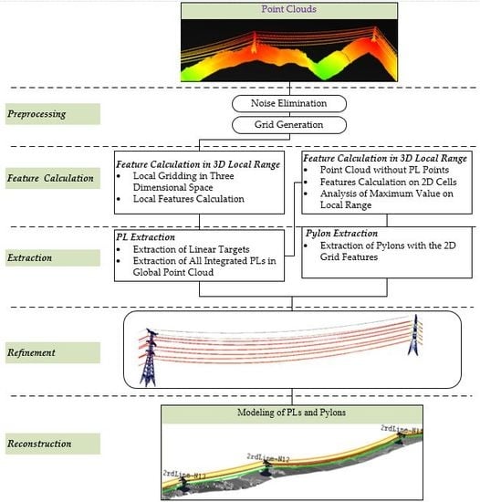
Figure 1 illustrates the whole workflow of the proposed method, which consists of five steps: data preprocessing, feature calculation, object extraction, optimization, and reconstruction.

• Preprocessing. The first step is to remove the sparse noisy points and divide the data into grids at different levels. First, 5 × 5 m² grids were constructed in the 2D horizontal plane considering the horizontal diameter of HV pylons, then were further divided into 0.5 m³ voxels for detailed analysis. The grid structure contains not only the point set within its range, but also grid features including the values of height difference, inclination, and point density within the grid.
• Dimensional feature generation. Based on the analysis of several geometrical distribution features of transmission lines locally (linear, parallel, consistent) and globally (elongate), PLs were extracted using 3D grid features; four further features were then extracted based on 2D grids, i.e., large height difference, continuous height distribution, local extremely high value, and limited range in planar projection map, were calculated to differentiate pylons and poles from the other objects.
• Extraction of individual lines and towers. First, PL segments were labeled based on the local linear geometric distribution in 3D. Consecutive PL segments were then merged as PL candidates. Next, the HV pylons were detected using the 2D grid features calculated above within the whole strip of the scanned transmission corridor.
• Optimization. The preliminary result was optimized by a feature of positional relationship between the HV towers and PLs in the 3D space, on the basis that they successively connect to each other around individual lines at the point of attachment (POA) [40].
• Reconstruction. The 3D PL was modeled using a 2D line in a projected ground plane and a catenary curve in the vertical plane that is perpendicular to the projection plane. The pylons were constructed by fitting with models from an existing library.

3.1. Preprocessing

Traditional point cloud data management and search methods are often computationally costly [55,56]. Therefore, in this paper, PLs were segmented by means of data partitioning based on a memory- and computing-efficient data structure.

Planar compression and hash storage scheme: The voxel grid was set as the unit to organize by the hashing storing scheme, which contains the index of all voxels. The spatial hash [57,58,59,60,61,62,63] data structure dealt with the voxels of observed space by marking them in the hash table with a pointer stored in it. Additionally, structured data can be read and written effectively, allowing for faster calculation of features [64]. The grid blocks were stored using this scheme, combined with the sparse matrix. Unlike conventional or hierarchical grid data structure, this 3D hashing matrix can substitute memory intensively and can compactly deal with sparse grids (grids that contain few points). In fact, many grids did not contain laser points; they conformed to sparse matrix logic [65], and thus were stored in the spatial hashing structure which sparsely and efficiently managed compressed point clouds in grid blocks. Consequently, a large number of data-free grids were eliminated to save memory. The processing with 3D grid as the unit improved the efficiency of the subsequent clustering for local PL segmentation.

2D grid generation: Due to the high volume, high density, and unordered distribution of the point cloud data, planar 2D gridding was exploited to manage the contextual features. Local grid features (the density and height at the level of individual grid) were calculated during the process of planar gridding, which facilitated the rapid identification of HV pylons candidate areas. First, the distribution range of the original points was computed to estimate the number of grids [66]. Each point was re-calculated with regard to the new planar coordinate system to allocate it to its grid. The process iterated until all points were allocated. The formula used is as follows:

$$\{\begin{array}{c}\mathrm{m}=\left(\mathrm{y}-{\mathrm{y}}_{\min }^{\mathrm{G}}\right)/\mathrm{d}2\\ \mathrm{n}=\left(\mathrm{x}-{\mathrm{x}}_{\min }^{\mathrm{G}}\right)/\mathrm{d}2\end{array},$$

(1)

where (x, y) refers to the candidate horizontal coordinates, ${\mathrm{x}}_{\min }^{\mathrm{G}}$ represents the minimum value of the x-coordinate in the overall point cloud data, ${\mathrm{y}}_{\mathrm{m}\mathrm{i}\mathrm{n}}^{\mathrm{G}}$ refers to the minimum y-coordinate, $\mathrm{d}2$ represents the size of the planar grid, and m and n are the row and column numbers corresponding to the grid where the point is located.

Voxel Hashing: The 3D hashing scheme stores 2D grids in the beginning. Subsequently, in each 2D grid, new coordinates of each point are calculated during the dynamic update of voxels with regard to hashing voxels, as follows:

$$\{\begin{array}{c}\mathrm{r}=\left(\mathrm{y}-{\mathrm{y}}_{\min }^{\mathrm{L}}\right)/\mathrm{d}3\\ \mathrm{c}=\left(\mathrm{x}-{\mathrm{x}}_{\min }^{\mathrm{L}}\right)/\mathrm{d}3\\ \mathrm{h}=\left(\mathrm{z}-{\mathrm{z}}_{\min }^{\mathrm{L}}\right)/\mathrm{d}3\end{array},$$

(2)

where $\left(\mathrm{x},\mathrm{y},\mathrm{z}\right)$ represents the 3D coordinate; ${\mathrm{x}}_{\min }^{\mathrm{L}}$ represents the minimum value of x-coordinate within the grid; ${\mathrm{y}}_{\min }^{\mathrm{L}}$ represents the minimum y-coordinate within the grid; ${\mathrm{z}}_{\min }^{\mathrm{L}}$ refers to the local minimum z-coordinate within the grid; d3 refers to the 3D voxel grid size; and $\mathrm{r},\mathrm{c},$ and $\mathrm{h}$ are the row, column, and height corresponding to the points in the 3D grid, respectively. The voxel was built based on the planar grid as a parent unit, and the size of the voxel grid was determined by the 3D spatial distribution and the voltage level of the HV wires (e.g., the offset of adjacent lines or voltage classes should be taken into account). To balance computation efficiency and feature accuracy, 0.5 m was set empirically as the size of voxel. 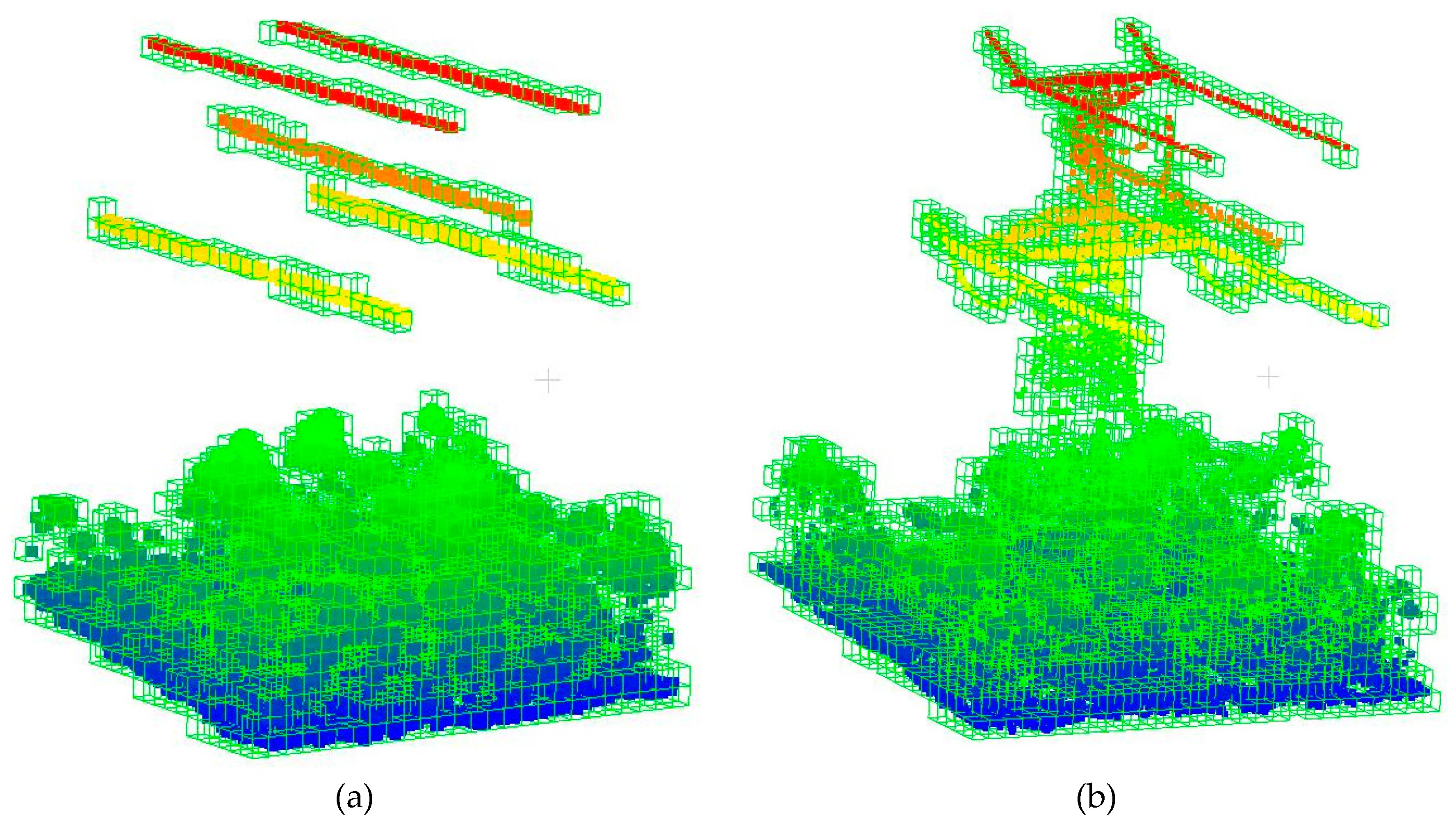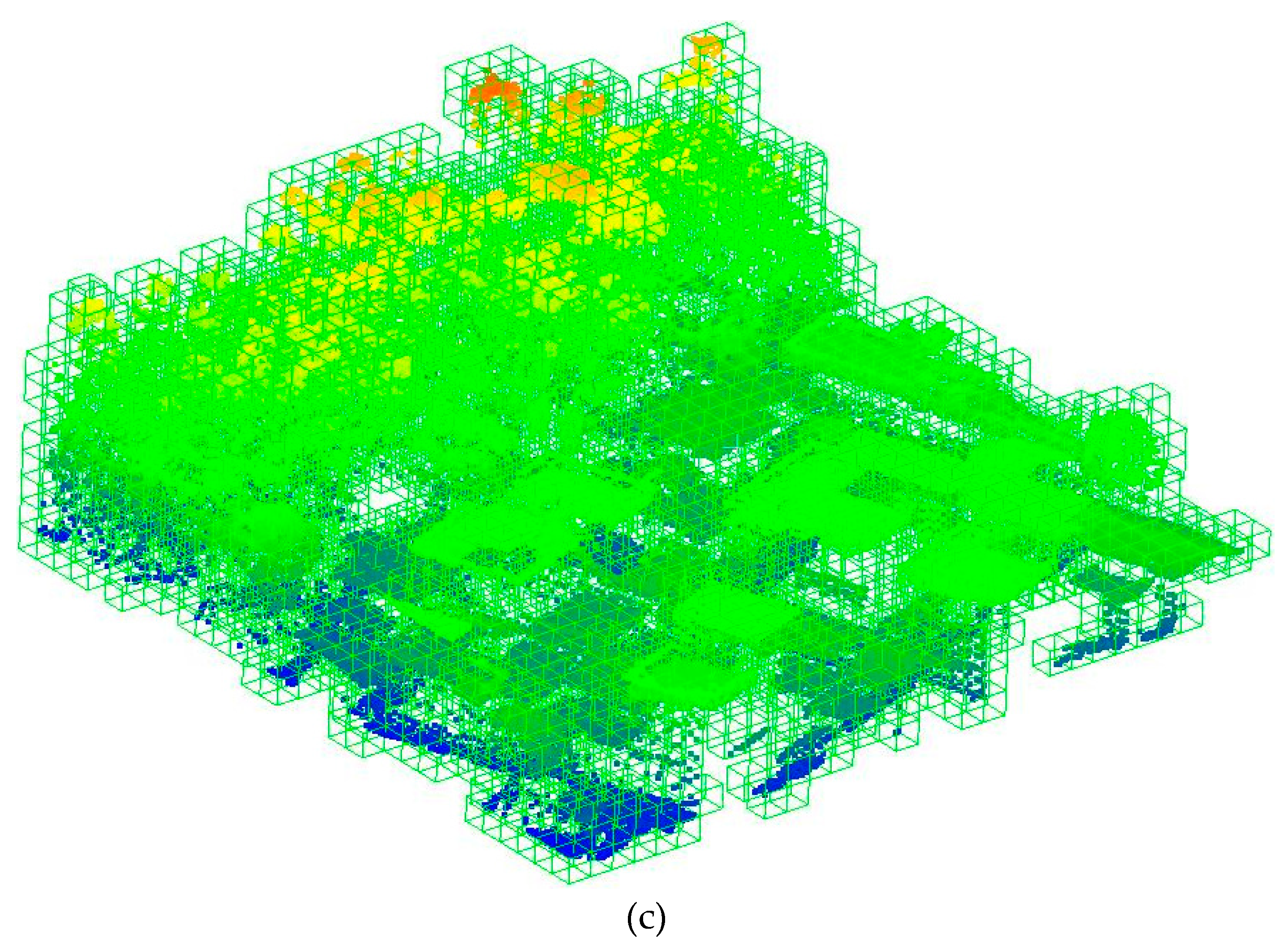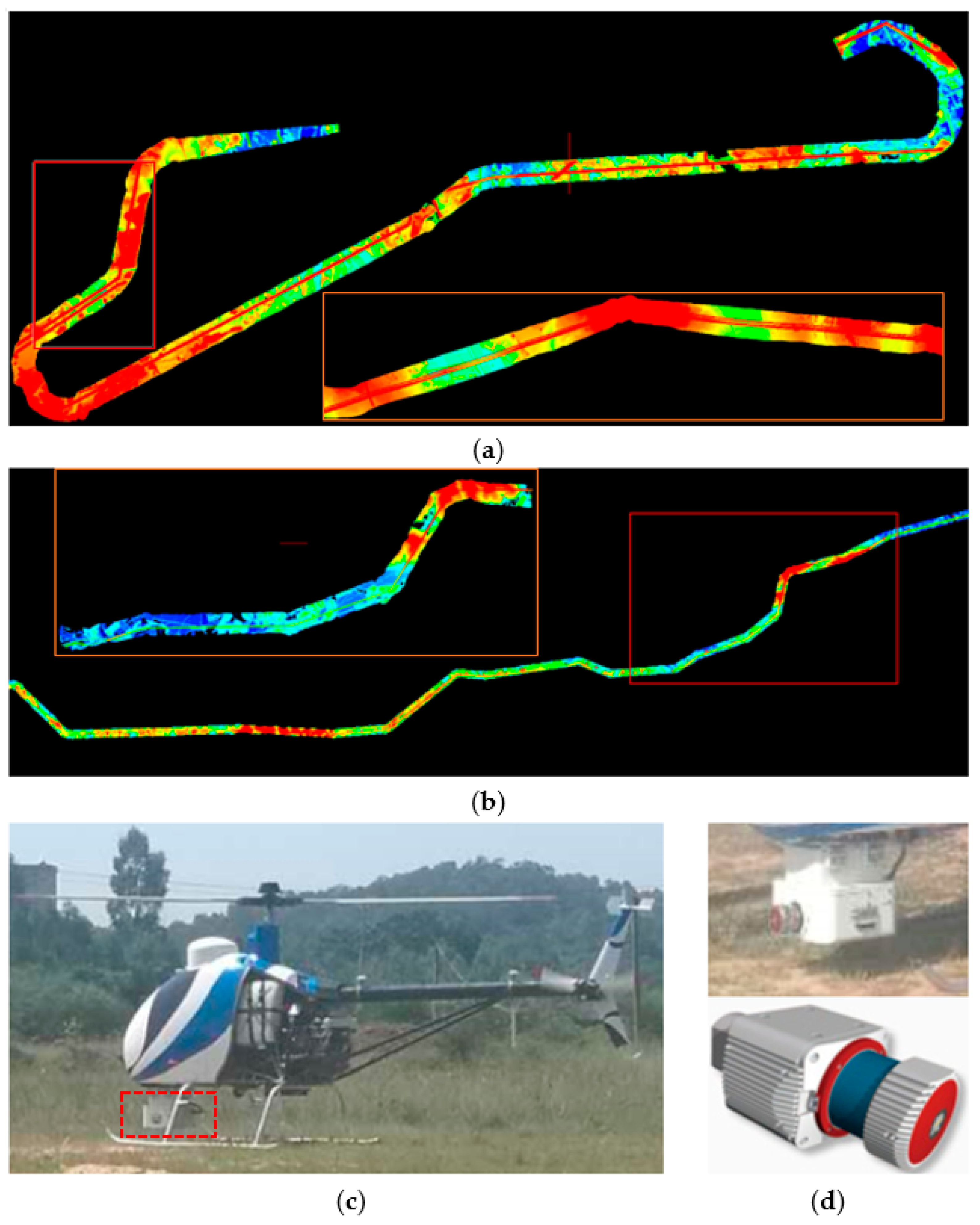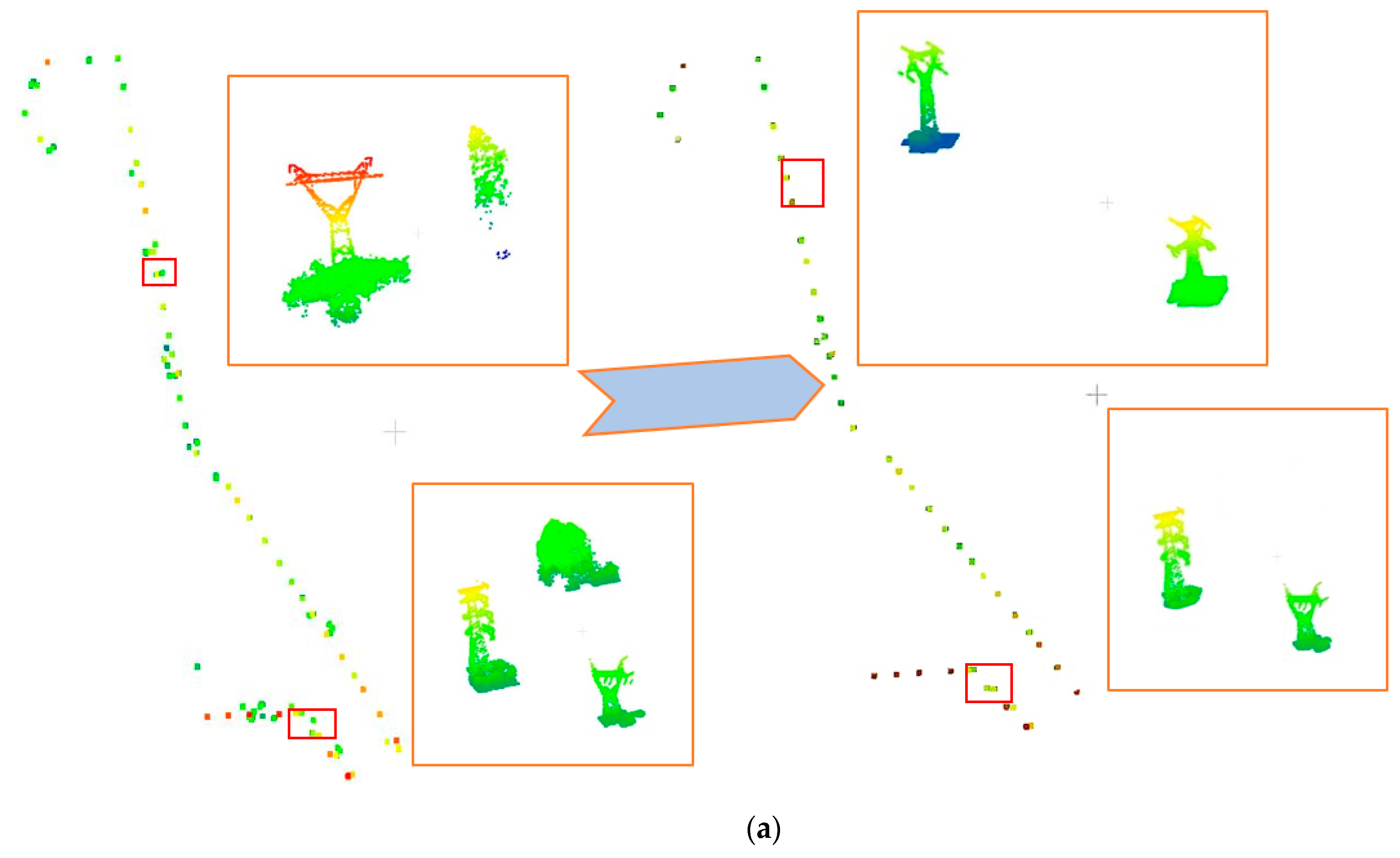Figure 2 shows the results of the PL and pylon voxel blocks and blocks without power transmission objects.

3.2. Feature Calculation

In order to extract the transmission objects, different features of PLs and pylons, i.e., dimensional features (eigenvalue-based) and distribution features (point-based) of the point clusters were utilized. The distribution features consisted of height features (e.g., local digital elevation model (DEM), digital surface model (DSM), and height difference) and density features.

Feature calculationin 2D grids: The terrain where power transmission lines are constructed is generally uneven. Nevertheless, power pylon points normally have large height differences and continuous vertical distributions, and their height values tend to be high [67]. These properties of distribution are not affected by the terrain and surrounding objects, providing a strong basis for pylon identification.

Considering a grid as a unit, features of point data in each grid were calculated, including DEM, DSM, and height-difference. Among them, DEM and DSM were obtained directly through statistical analysis of the point cloud. The height difference was calculated by subtracting DEM from DSM. Notice that the PL points extracted earlier from the corresponding point cloud data should be separated out when the grid-based DSM features are computed.

DEM reflects the distribution of topographic relief in the mapping area. The adverse impact of topography fluctuation on pylon extraction can be suppressed by normalizing the DSM using DEM. Normalized DSM (nDSM) reflects the local height differences within the point cloud data. Because of the large height difference of HV towers, the pylons are easily visible in nDSM.

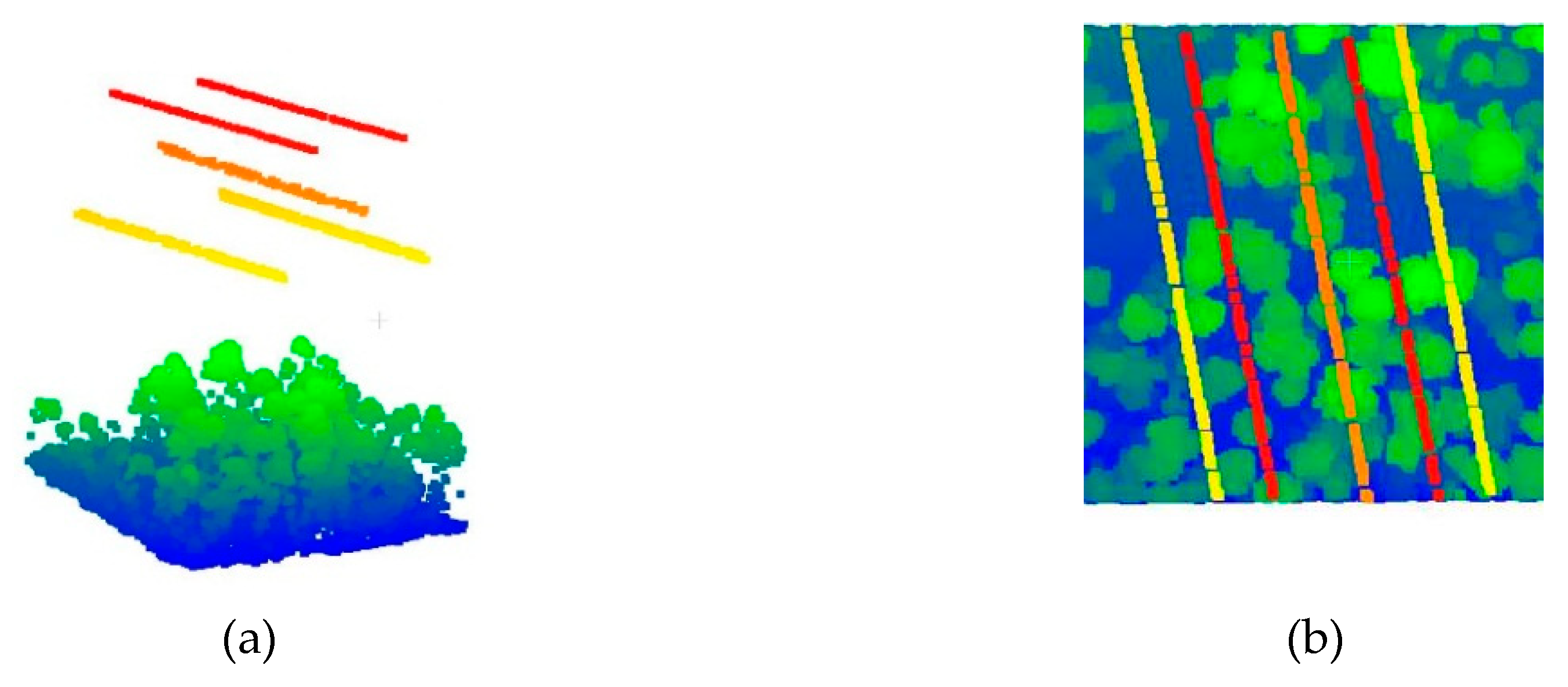
3D feature calculation: According to Kim et al. [41] and Melzer et al. [27], PL points have the properties of local linearity and consistency of local convergence, which can be used to distinguish PLs from other objects. In Figure 3, these dimensional features can be intuitively observed. Points in each 2D grid were first clustered based on Euclidean distance, then the voxels in each cluster were taken as a basic unit to calculate the dimensional features of points. By computing the covariance matrix [7] and the eigenvalues of all points in the clustered voxels, the linear, planar, and spherical features were derived. The linear structure of a point set was determined by comparing the three values ${\mathrm{a}}_{1\mathrm{D}}$, ${\mathrm{a}}_{2\mathrm{D}}$, and ${\mathrm{a}}_{3\mathrm{D}}$, calculated as:

$${\mathrm{a}}_{1\mathrm{D}}=\frac{\sqrt{{\mathsf{\lambda }}_1}-\sqrt{{\mathsf{\lambda }}_2}}{\sqrt{{\mathsf{\lambda }}_1}},{\mathrm{a}}_{2\mathrm{D}}=\frac{\sqrt{{\mathsf{\lambda }}_2}-\sqrt{{\mathsf{\lambda }}_3}}{\sqrt{{\mathsf{\lambda }}_1}},{\mathrm{a}}_{3\mathrm{D}}=\frac{\sqrt{{\mathsf{\lambda }}_3}}{\sqrt{{\mathsf{\lambda }}_1}},$$

(3)

where ${\mathsf{\lambda }}_1$, ${\mathsf{\lambda }}_2$, ${\mathsf{\lambda }}_3$(${\mathsf{\lambda }}_1$ > ${\mathsf{\lambda }}_2$ > ${\mathsf{\lambda }}_3$) [68] refer to the eigenvalues of the covariance matrix of each point set.

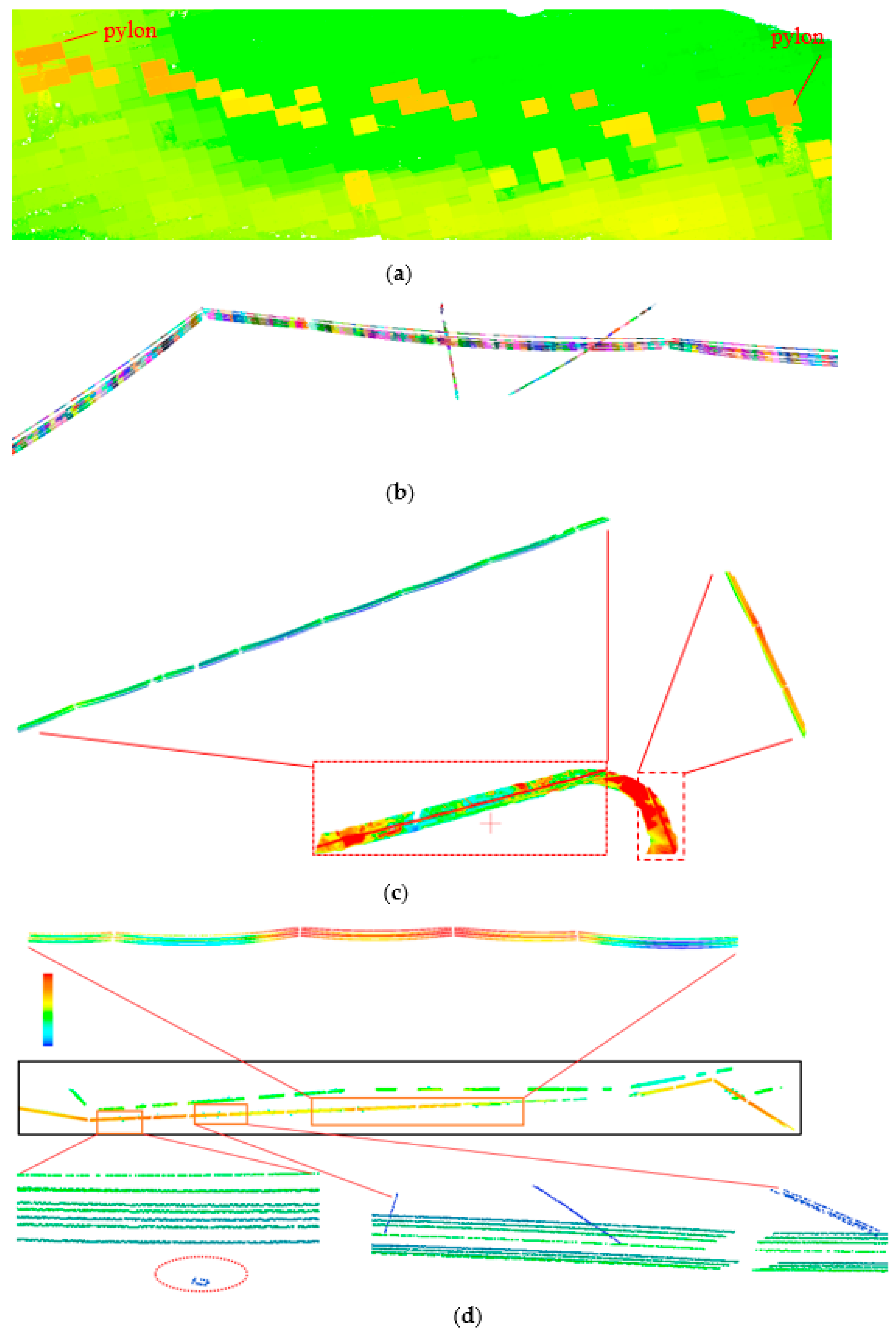
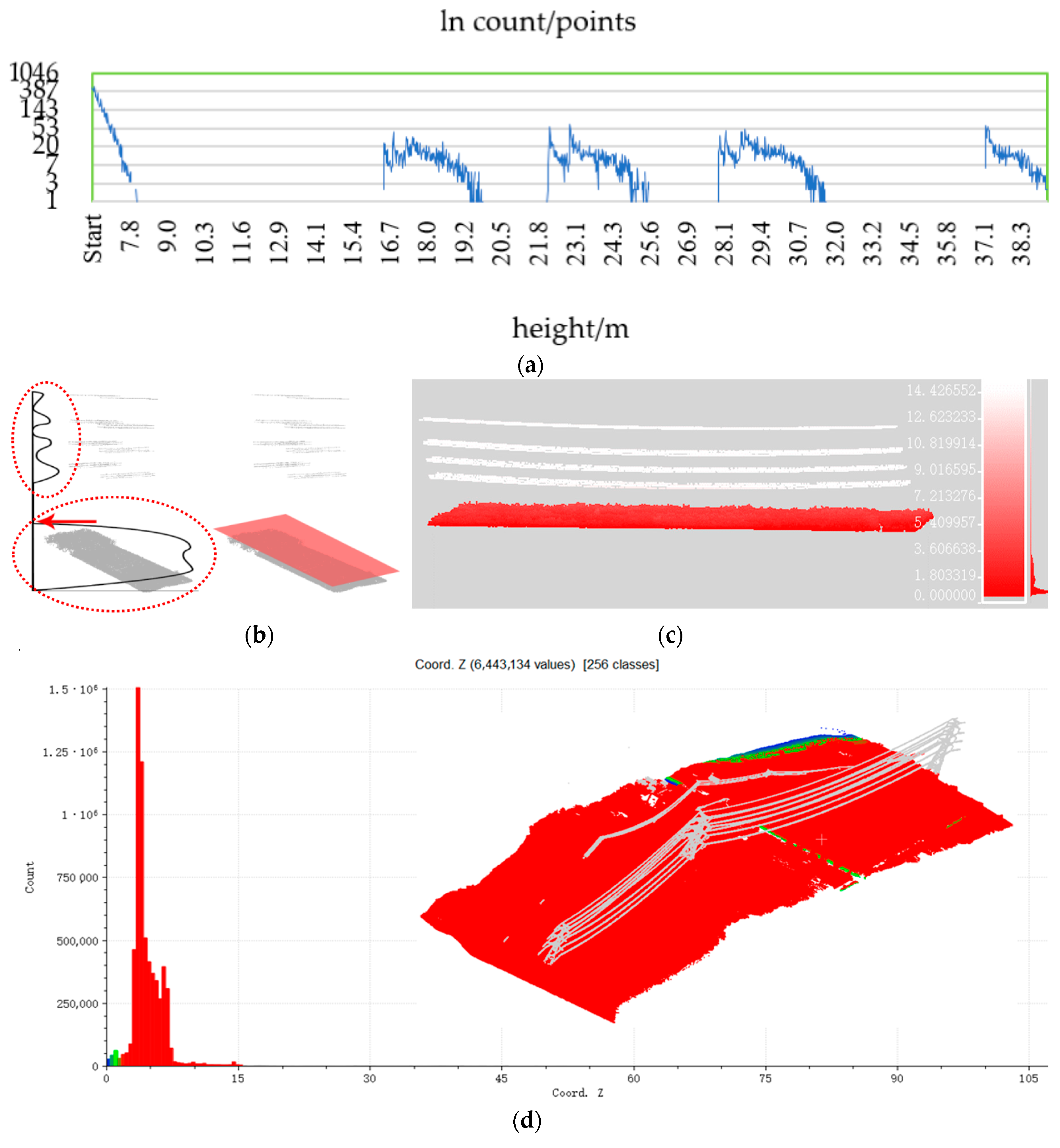
Height distribution: By analyzing the patterns shown in Figure 4, it can be obviously seen that the relative height and local linearity are features able to distinguish PLs from other objects. The clustering distance is indicated by the distance calculated by the height distribution feature. The value is the minimum height gap from an overhead PL to the ground objects in a span (the space between two adjacent pylons). Using the height distribution histogram (Figure 4b) of a test dataset in Figure 4a, where the points above 13 m are highlighted, the gap was fixed at the height of about 8 m. The gap between the first and the last peak was considered similar to the height of the top area of a tower, named as the head of the tower.

3.3. Segmentation of Power Lines and Pylons

The main components of HV power transmission corridors include PLs, pylon insulators, fixed accessories, etc., of which the key parts are the transmission lines and pylons (also called towers). Based on the spatial stratification of the corridor and the features of PLs discussed above, PLs were segmented first. HV pylons were then recognized by their properties in vertical and horizontal distributions without considering PL points.

3.3.1. Power Line Extraction

According to the abovementioned features of the geometric spatial distribution of overhead PLs, they were extracted in two steps: local line segment extraction based on dimensional features, and global PL merging based on local collinearity and height approximation. The key was to search for linear and parallel structures exceeding the minimum height interval in clustered point sets.

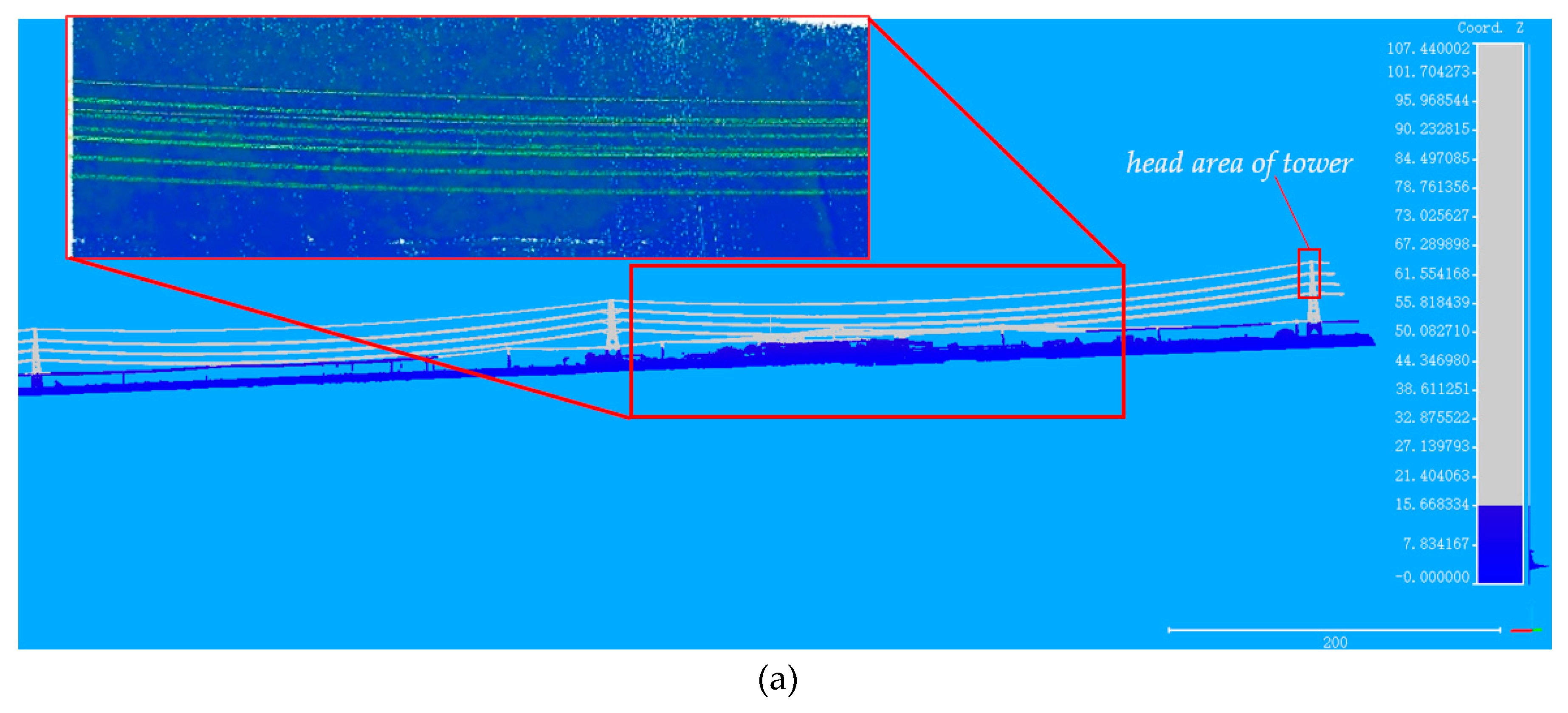
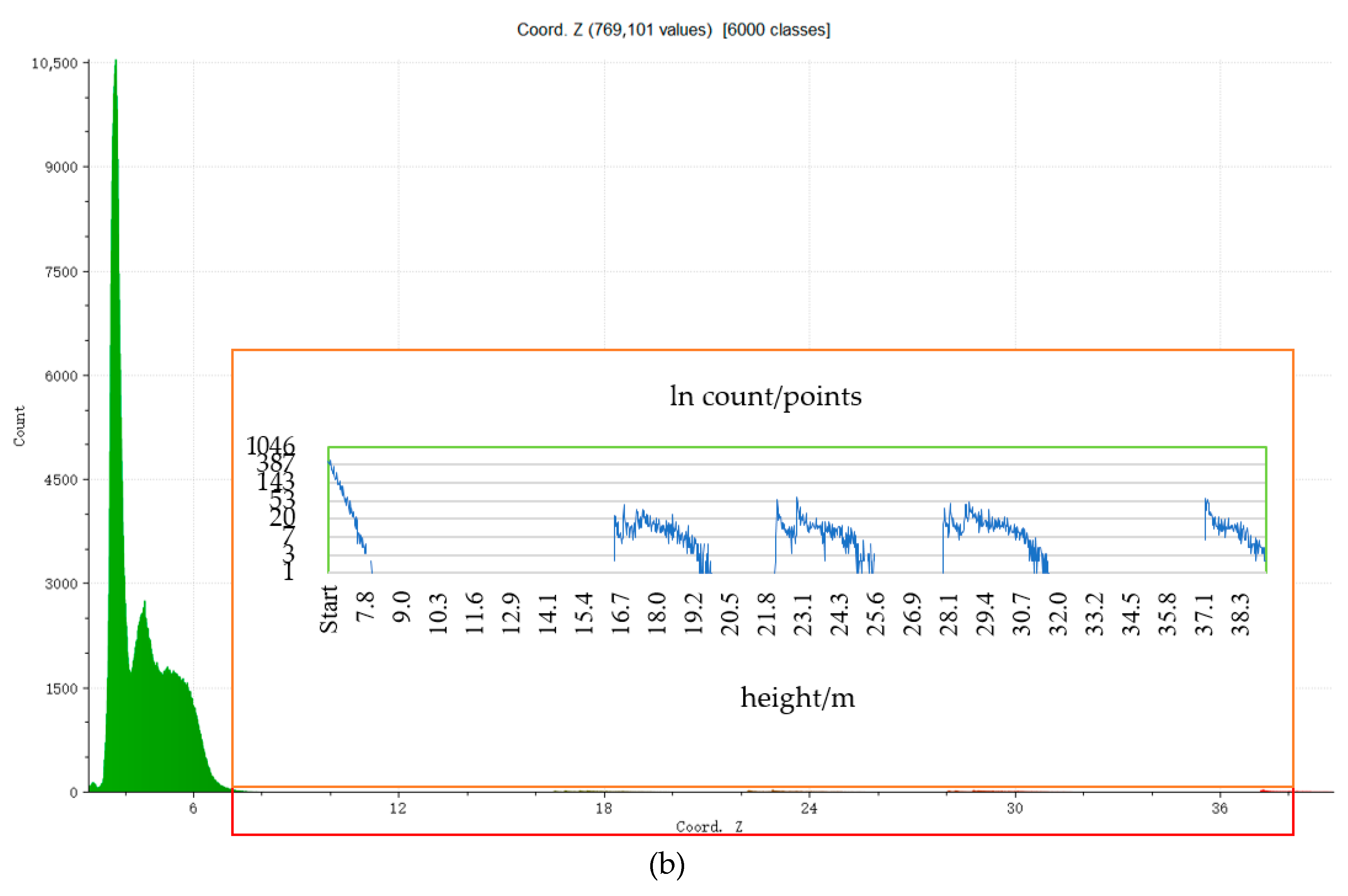
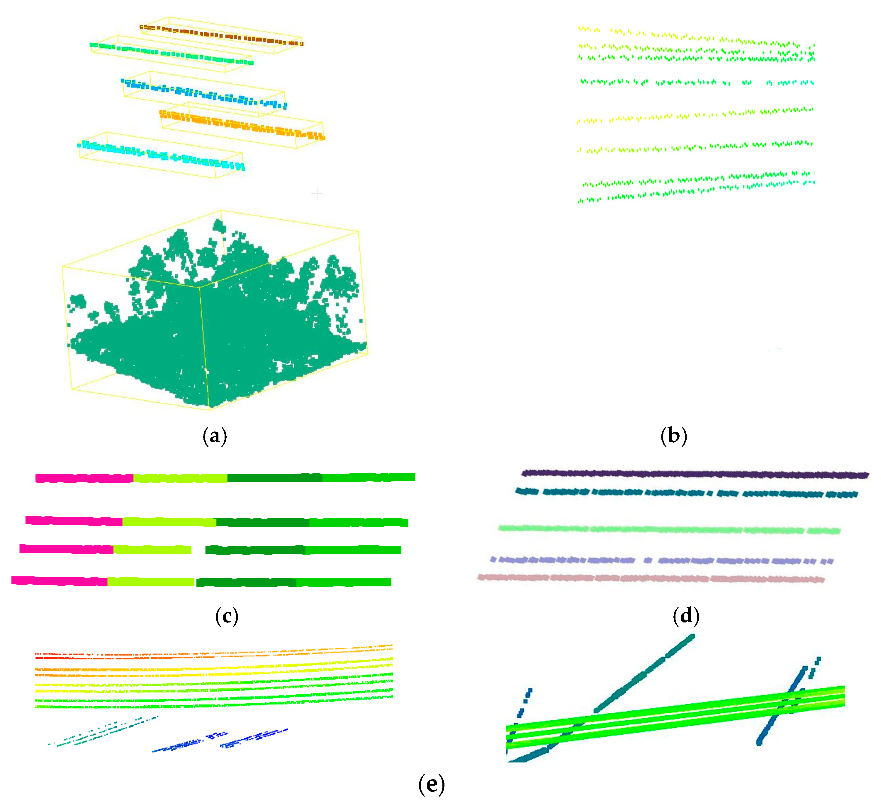
Local segmentation: The local segment extraction was carried out by judging the dimensionality of clustered point set—whether it had a linear feature. The next step was to search for linear structures among neighbors by eigenvalues, i.e., a neighborhood cluster search. The retained results, including linear structure, were seen as candidate PL segments. To visually demonstrate the effectiveness of the algorithm, Figure 5 shows the segmentation result of part of the input data. The resulting linear segments were then pushed to the memory to extract PLs globally.

PL segments detected within a cluster of voxel blocks were recognized as parts of different PLs. As shown in Figure 5, they did not overlap by local linearity analysis. By this property, a randomly selected seed segment was clustered with segments in neighbor blocks. Each segment was independent of the others, and the calculation in each span was independent. To improve the computation efficiency, this part can run in parallel.

Global extraction: After extracting the candidate PL segments, as shown in Figure 5c, the local collinearity of the adjacent PL segments was analyzed to get complete lines. The whole PL extraction based on local collinearity was achieved by point cloud clustering in the horizontal domain, where the cluster unit was the PL segment, and the constraint was spatial continuity and local collinearity. Meanwhile, a CLF (compass line filter) [1,68] was applied to analyze the line direction using PL candidate points.

In the process of clustering, each 2D grid calculated above was set as the center unit, and the PL segments within its eight neighborhoods were searched to merge with seed PL segments located in the center grid. For linear segments aligned with the principle direction of the seed line segment, collinearity with the seed segment was assessed to eliminate those belonging to other, adjacent PLs. Figure 5d shows the extraction results within a span.

Shown in Figure 5e, the detected PLs may include low-voltage transmission wires that cross underneath. Cross-over or short-spanned low-voltage conductors were detectable, but were not the object of interest. Further optimization by combining with HV tower extraction is detailed in Section 3.4.

3.3.2. Regional Segmentation of Candidate High-Voltage Towers Based on 2D Features

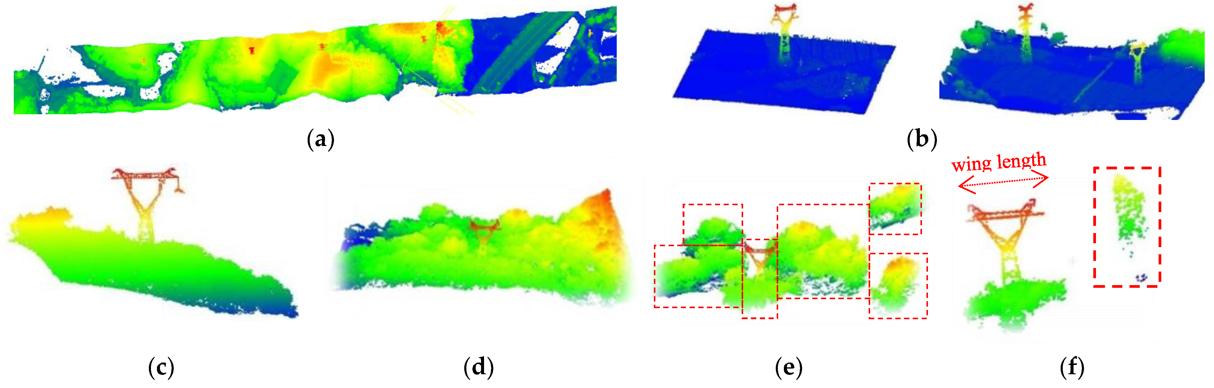
HV pylons, which support the transmission lines, sit on the ground, as shown in the point cloud data. Therefore, they show a continuous distribution in the vertical direction. Furthermore, according to the regulations governing overhead transmission lines, they must maintain a safe clearance to the surroundings or ground objects, so HV pylons are generally built more than 20 meters high. Figure 6 illustrates the characteristic of large local height difference in the areas where the HV towers are located. In the horizontal direction, the wing length of the HV pylons is related to the corresponding voltage level of the PLs. Given the voltage level, the distribution range of pylon points on the horizontal projection plane should be finite, as in Equation (4).

R_{(m, n)} ≤ (r + 5),

(4)

where R_{(m, n)} is the radius of the pylon candidates in the projected ground plane and r is the wing length. These distribution features of HV pylons were utilized to divide the candidate pylon areas.

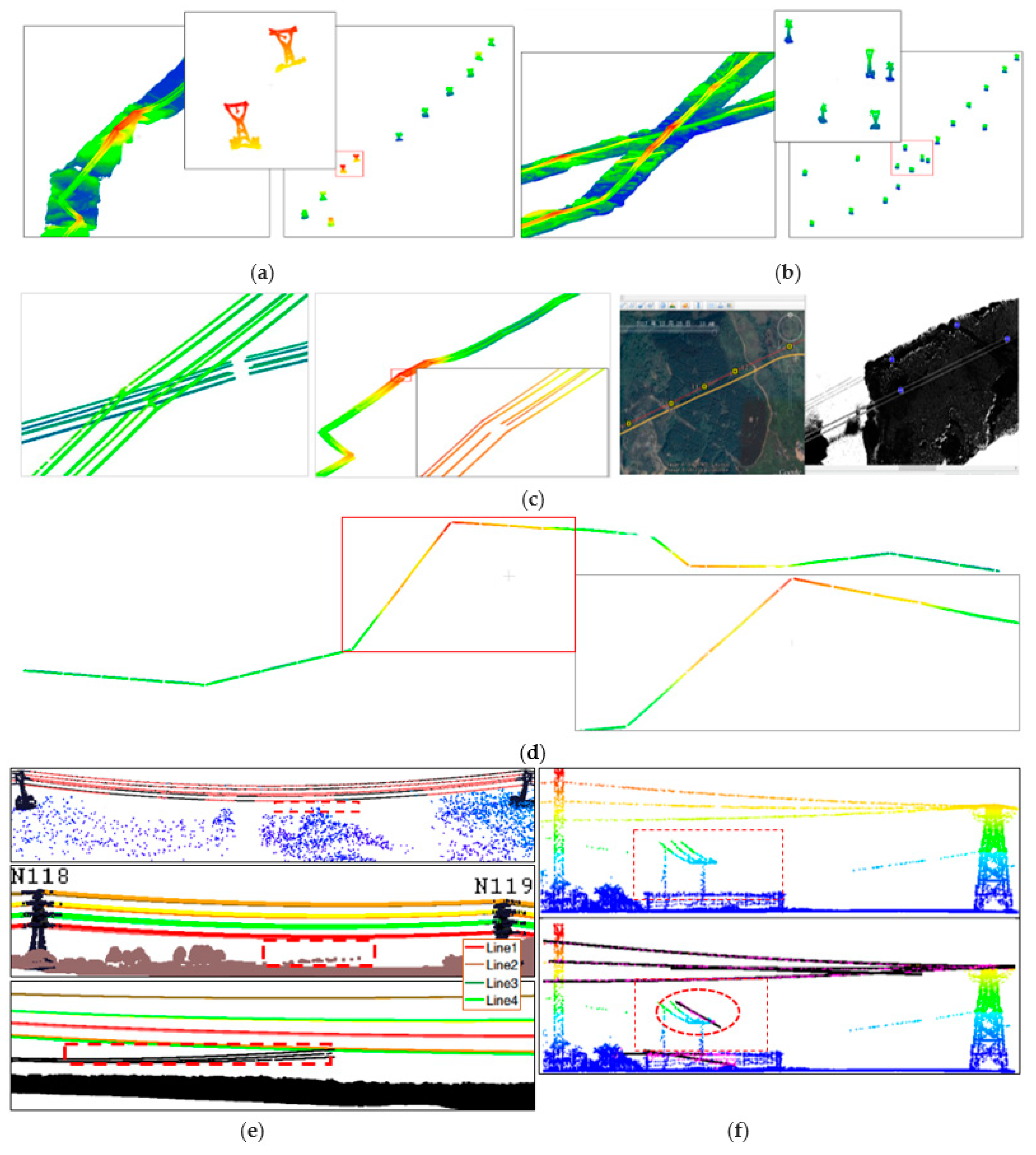
The segmentation was composed of five steps:

• The 2D grids of large height difference in the input data were first identified according to the height difference feature. As seen in the red dashed boxes in Figure 6e, these grids mainly consisted of towers, individual tall trees, or groups of clumped trees.
• A 2 × 2m grid was created as a moving window to detect the finer characteristics of the grids with large height differences. The window was initialized with the same features as the grid. When it moved, its features were updated. The height difference value of the moving window that was greater than the pre-defined threshold (the minimum height difference between PLs and the ground from previous analysis) was retrieved and the corresponding grid was marked.
• The vertical continuity of the points in each marked grid was checked. Given the maximum height gap threshold (usually set as the absolute height of the tower), grids containing a window of a higher gap than the threshold were removed to filter out outliers.
• The remaining grids were clustered to group the grids belonging to the same tower. Neighboring grids were clustered when their height differences were greater than the pre-defined threshold.
• The distribution range of HV pylons in the planar projection was utilized to differentiate them from other clustered objects. The principal direction of each cluster was calculated. The semi-major axis of a tower in the planar projection range in the principle direction was not greater than the length of HV tower’s wing. From the horizontal projection range described by Equation (4), blocks of clumped trees were filtered out because their distribution ranges in the planar projection failed to meet the equation in the horizontal plane. Small clusters (see the dashed box in Figure 6f) were then excluded by judging whether each grid in the clustering blocks had an extremely local high value in the DSM feature map.

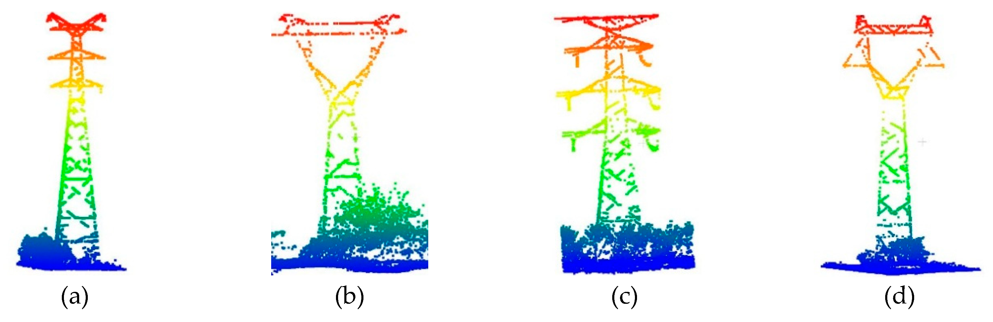
Figure 6a shows one dataset in which PL points were removed, and Figure 6b–d shows the top view and side view of some pylon areas. As a result of the extraction of pylons, points on the majority of non-power transmission components and tall clumped trees and arbors were removed. As can be seen from the result in Figure 6f, by extracting the grids with large height differences, most non-tower points were removed and the target tower was completely retained.

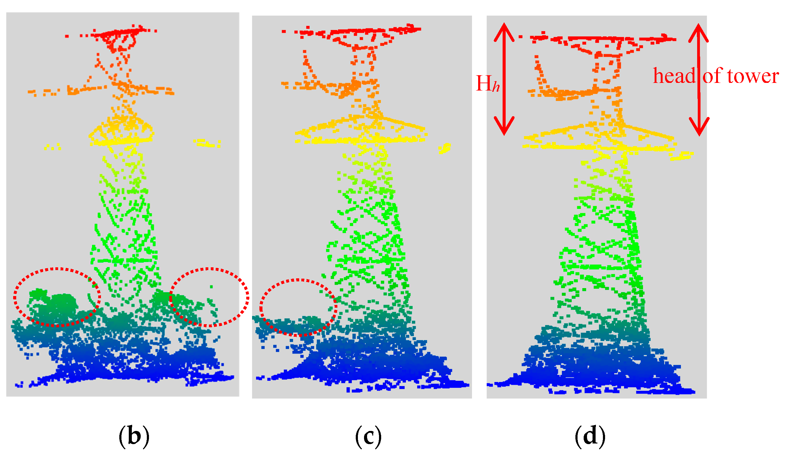
3.4. Optimization of the Extraction of Power Transmission Components

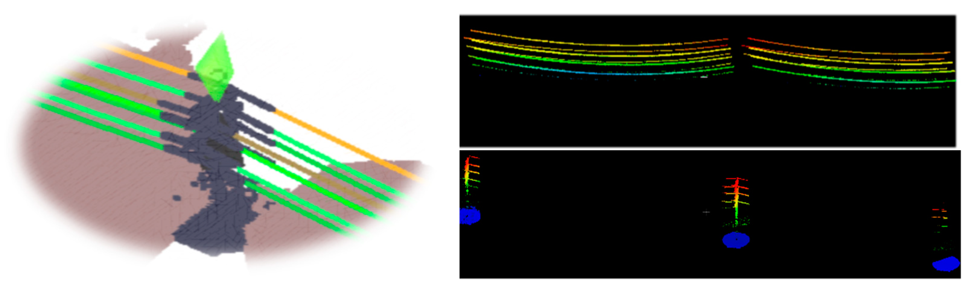
After PL and tower detection, a few single tall trees, signal poles (happened to be in the corridor) and low-voltage PLs were still present in the scene as interference factors. However, in the transmission corridor, any PL was hanging in midair in the 3D space and was connected with HV pylons. This constraint was used to refine the pylon and PL detections. As seen in Figure 7, pylon and PL points were connected to each other, which is a unique feature that can be used to distinguish HV towers from interference elements. Note that HV transmission lines were different from other linear interference factors such as low voltage conductors or supporting wires. Additionally, as a basic criterion, the principal direction of the candidate PL points was approximately parallel to the line connecting their two adjacent towers [69].

Thus, the extractions of those two transmission objects were optimized simultaneously, considering the physical connections between them. This included the following constraints: (a) the transmission tower and the PLs were connected to each other [27], meaning the PLs in neighbor spans were connected through the HV towers; (b) the dominant orientation of the PLs was approximately parallel to the line connecting the towers at both ends; (c) the neighboring grid of the tower must contain PLs, and there should be a tower at the position of the derivative extremum of each adjacent line.

• First, the extracted HV towers were taken as searching objects. For each HV tower, the neighboring grids were searched for PL points.
• Secondly, the PL point set and the tower were confirmed to be connected to each other. If a tower was connected with a PL, it was determined as HV tower area, and the PL connected with it was labeled as transmission wires.
• Lastly, the directions formed by every two adjacent pylons were taken as references to remove the linear segments with large angles from these directions.

The above steps eliminated tall trees, signal poles, and other remaining interferences of low-voltage transmission wires and other linear targets. Illustrated in Figure 8b,c, tree points with a similar distribution of pylons, and most low-voltage transmission lines and cross-over transmission lines (see in Figure 8a), were excluded. As depicted in Figure 8d, the result was the clean and complete detection of PLs and pylons in a span.

3.5. Reconstruction of Power Transmission Components

3D reconstruction of PLs is the basis for the applications of transmission corridor safety inspection, 3D scene visualization, and condition monitoring. Generally, the PLs are divided into individual fixed-length lines according to the POAs, to facilitate the line fitting.

3.5.1. Modeling of Power Lines

Through spatial connectivity analysis of adjacent transmission lines, the integrity of lines was guaranteed and the relationship between lines and towers was determined [51]. The PLs were split into spans formed by adjacent towers. The 3D PLs were reconstructed on the assumption that they were flexible free-hanging wires that could be expressed by a mathematical model [70]. The 3D model was described by a straight line using least squares in the horizontal plane and a catenary in the vertical plane. The PLs in each span were modeled separately. They were then combined with the models of pylons. The mathematical model demonstrated by Jwa and Sohn [30] was separated into a catenary (Equation (5)) and a line (Equation (6)). Equation (5) is solved by minimizing the difference between the observed Z value and the fitted Z value of points in each segment, as in Equation (7).

$$\mathrm{C}\left(\mathrm{a},\mathrm{b},\mathrm{c}\right):\mathrm{Z}=\mathrm{a}\mathrm{c}\mathrm{o}\mathrm{s}\mathrm{h}\left(\frac{\mathrm{x}-\mathrm{b}}{\mathrm{a}}\right)+\mathrm{c},$$

(5)

$$\mathrm{L}\left(\mathsf{\theta },\mathsf{\rho }\right):\mathsf{\rho }=\mathrm{X}\cos \left(\mathsf{\theta }\right)+\mathrm{Y}\sin \mathsf{\theta },$$

(6)

$${\mathrm{C}}^{\prime }=\arg \underset{\mathrm{m}}{\min }{\displaystyle \sum }_{\mathrm{i}=1}^{\mathrm{n}}{\left[\frac{\mathrm{f}\left({\mathrm{x}}_{\mathrm{i}},\mathrm{m}\right)-{\mathrm{y}}_{\mathrm{i}}}{{\mathsf{\sigma }}_{\mathrm{i}}}\right]}^2,$$

(7)

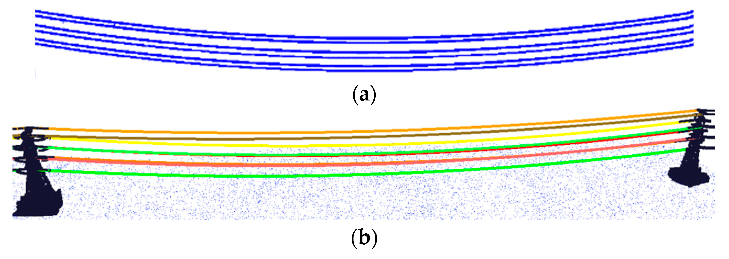
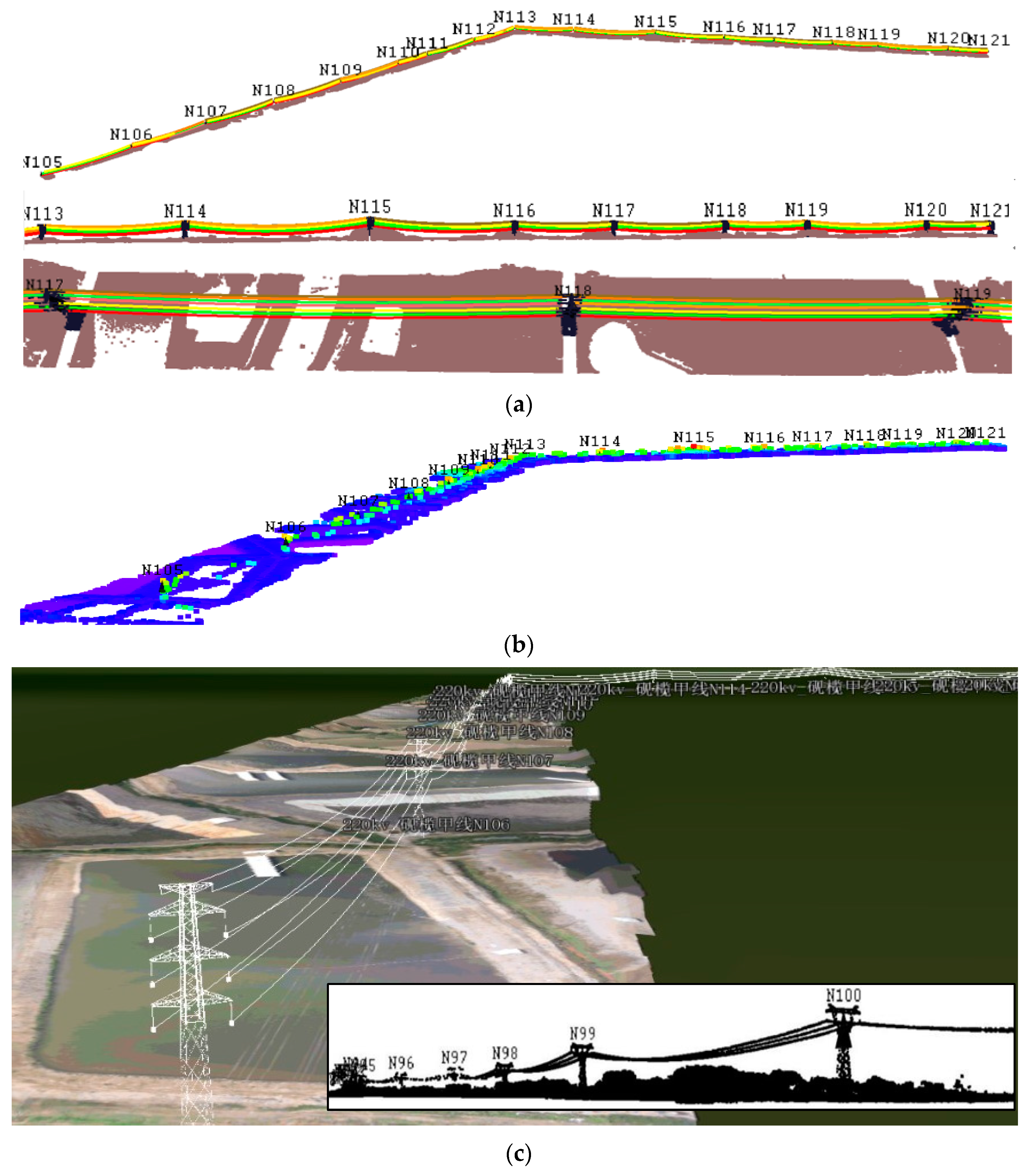
The Random Sample Consensus (RANSAC) algorithm was used to iterate each line point and rectify the fitted model using ever-increasing inner points to reconstruct each single PL. Figure 9a shows some exemplary fitting results of PLs in a span. The PLs in each span were modeled and colored separately by their electrical phase (Figure 9b). They were then combined with the models of pylons.

3.5.2. Modeling of Pylons Based on Tower Center Localization

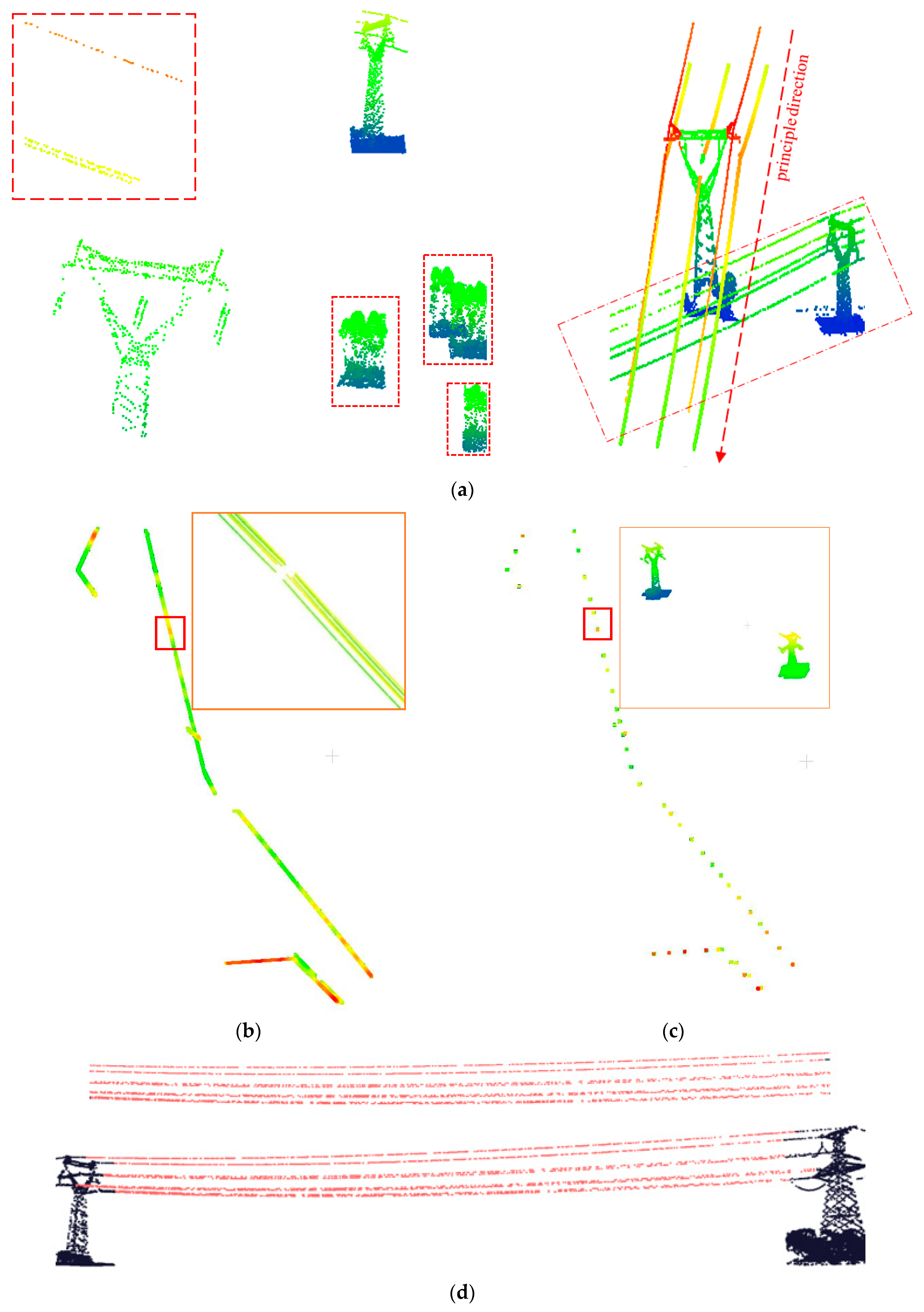
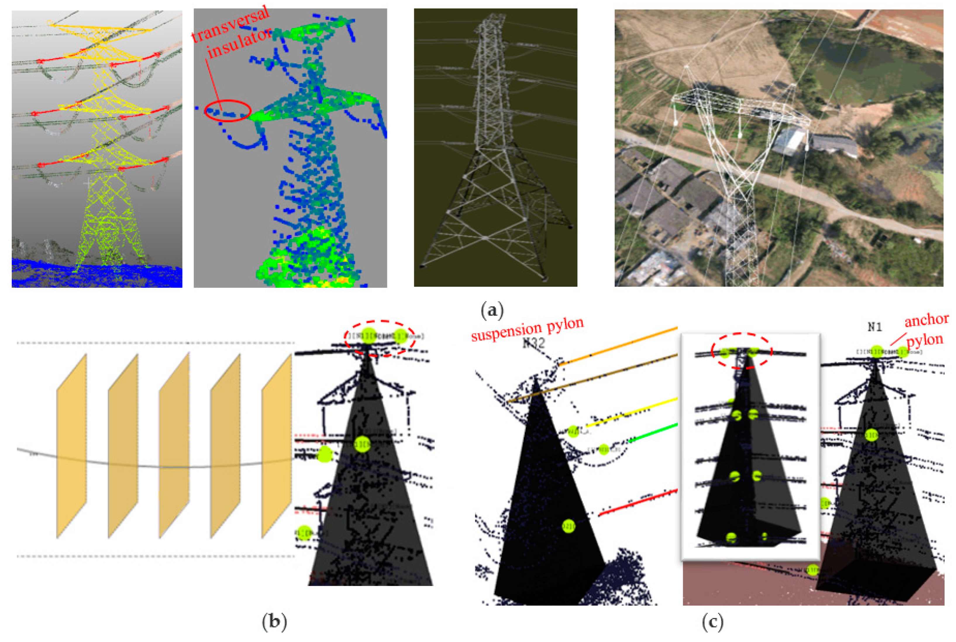
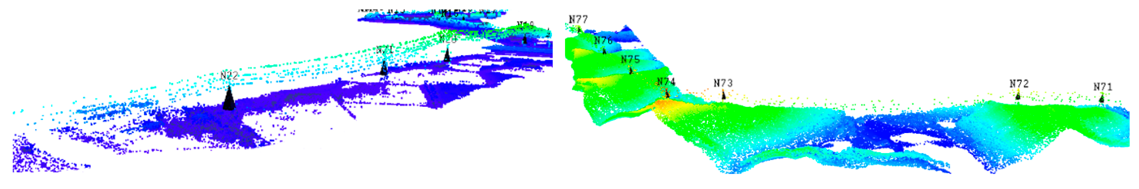
In the maintenance of power transmission, special attention should be paid to the stability of the HV pylons at a large scale and the accessories on them, i.e., the insulators and signs of tower number. Generally, the geographical coordinates of each pylon are required when dealing with the security of the transmission target. The main difference in this reconstruction approach is that we reconstructed not only the pylons, but also the insulators on them. First, the accurate planar coordinates of the pylons were calculated. Next, the library of tower templates was built according to the four basic types. Thus, the position error of the models built of each object in the corridor scene was smaller than others’ work. Moreover, the pylons were reconstructed as a whole model and were detailed by locating and modeling their insulators.

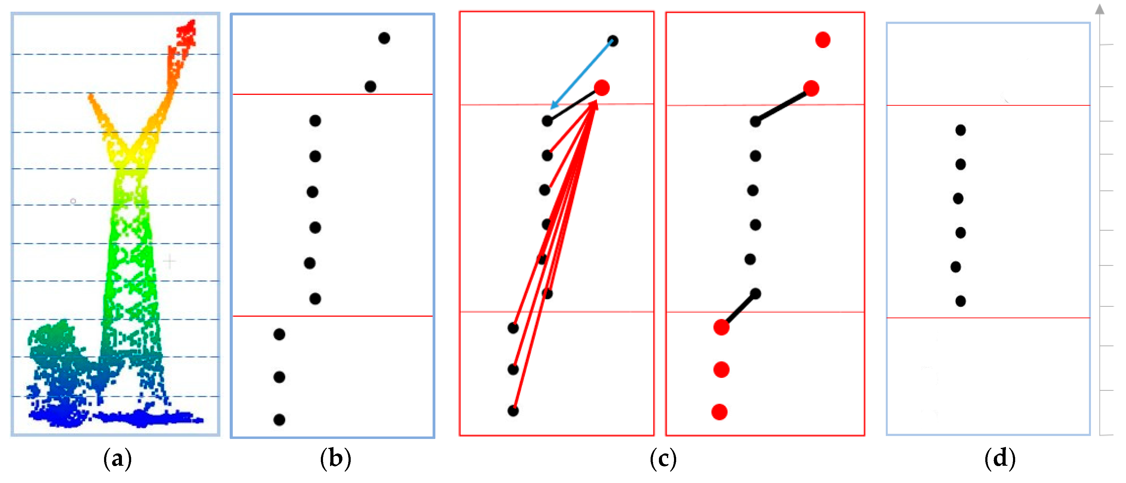
Planar Center Localization: Having identified the grids where the power towers are located, their structure and shape were abstracted to the four categories in Figure 10. Their distribution varied, which had an obvious influence on the plain projection feature of density and feature of height distribution. When calculating their central points, multiple voting mechanisms were used to search for the most reliable point centers of the horizontal section in multiple iterations.

As HV towers are regular to some extent, a horizontally sliced layer at any height of a tower body has an in-plane symmetry, as long as the points on the tower are not largely missing. The centers of those sliced layers based on the stratification in vertical direction can be used to calculate the accurate planar coordinates of the HV tower.

As shown in Figure 11a, there were still some vegetation points attached to the bottom of the tower, and the tower points were incomplete at the top. The central positions of the sliced layers shown in Figure 11b were also affected by the missing points. According to the verticality of the HV tower, there should have been a small angle between the vertical direction and the vectors formed by the centers of the layers (Figure 11c). The six points in the middle of Figure 11d describe the identified candidate central points, analyzed statistically by the algorithm shown in

Table 1. The tower center coordinate calculation algorithm.

$\mathbf{Input}:\mathbf{HV}\mathbf{Towers}\mathbf{in}\mathbf{Grids}{\mathit{M}}^{\mathit{c}}.$
Output: coordinates of HV tower centers
1.	Divide points ${\mathrm{C}}_{\mathrm{i}}$ in ${\mathrm{M}}_{\mathrm{i}}^{\mathrm{c}}$ into layers at a certain height gap (2 m). Calculate center points $\mathrm{P}$ of all layers. Take two adjacent layers ($\mathrm{P}\mathrm{i},\mathrm{P}\mathrm{i}+1$) as a pair, calculate ${\mathrm{d}}_{\mathrm{rc}}{\mathrm{and}\mathsf{\theta }}_{\mathrm{rc}}$.
2.	Query the maximum ${\mathrm{d}}_{\mathrm{M}\mathrm{r}\mathrm{c}}$ from {${\mathrm{d}}_{\mathrm{r}\mathrm{c}}$}; if ${\mathrm{d}}_{\mathrm{M}\mathrm{r}\mathrm{c}}$ > 0.5 m, then compute the $\mathrm{e}$ passing through ${\mathrm{p}}_0$ (another center point) and $\mathrm{e}$ and repeat this process to ${\mathrm{p}}_{\mathrm{c}}$.
3.	Vote for the one, ${\mathrm{p}}_{\mathrm{r}}$ or ${\mathrm{p}}_{\mathrm{c}}$, with larger ${\mathsf{\theta }}_{\mathrm{rc}}$ when each ${\mathsf{\theta }}_{\mathrm{rc}}$ is calculated. Delete the one with more votes from the two center points ${\mathrm{p}}_{\mathrm{r}}$ and ${\mathrm{p}}_{\mathrm{c}}$, and delete all ${\mathrm{d}}_{\mathrm{r}\mathrm{c}}$ and ${\mathsf{\theta }}_{\mathrm{r}\mathrm{c}}$ values relating to it, then go back to step 2.
4.	If ${\mathrm{d}}_{\mathrm{Mrc}}$ > 0.5 m, return the average coordinate values of the remaining center points coordavg.

, in which ${\mathrm{M}}_{\mathrm{i}}^{\mathrm{c}}$ is a collection of tower grid, which is then divided in to several layers ${\mathrm{C}}_{\mathrm{i}}$ 2 meters in height; ${\mathrm{d}}_{\mathrm{r}\mathrm{c}}$ is the horizontal distance of two center points; ${\mathsf{\theta }}_{\mathrm{rc}}$ is the angle between the z-axis and the line through the two central points determined by center point pairs, consecutively; ${\mathrm{d}}_{\mathrm{M}\mathrm{r}\mathrm{c}}$ is the maximum of collection {${\mathrm{d}}_{\mathrm{rc}}$}; and ${\mathrm{p}}_{\mathrm{r}}$ and ${\mathrm{p}}_{\mathrm{c}}$ are center points of the two layers corresponding to ${\mathrm{d}}_{\mathrm{M}\mathrm{r}\mathrm{c}}$.

Pylon modeling: In this paper, the methodology proposed by Li et al. [48] was applied to build the 3D pylon models, based on model fitting using a library of high-precision tower models built manually according to relevant specifications. The 3D model was initiated at the center of the detected tower, defined by the planar location and half of its height. The model size was determined by the voltage level when the power transmission was designed, as shown in Figure 12a. The Gibbs energy model was established to estimate point cloud and model fitness during the reconstruction process. Since the optimization process of the energy model was non-convex, the towers were reconstructed by energy optimization using Markov chain Monte Carlo (MCMC) [49].

Insulator modeling: Insulator reconstruction was achieved by insulator matching based on a region growing method. In most cases, it was fixed to a tower model [71]. Generally, insulator points were determined by contextual search and then clustered [21]. The insulator candidate points were searched within several successive adjacent vertical profiles in the principle direction of the PL (Figure 12b). In fact, insulator model construction was accompanied by the processes of line fitting and region growing along the vertical profile. The midpoint of the insulator point cloud was taken as the modeling center. For transversal insulators (points in the red ellipse in Figure 12a), the points located along the PL from its end until the center of the nearest tower were marked as insulator points. When the growth and fitting of the whole PL was completed, the insulator points on the corresponding line were also searched out. The yellow dots in Figure 12b were the centers of insulators. Note that the two (in the dashed ellipse) on the top were removed, as there was no insulator along the shielded wire. Finally, corresponding types of insulator models were added to the tower model.

4. Experiments and Analysis

4.1. Study Area and Experimental Data

The study area of the HV transmission corridor is located in Guangdong Province, China. It is a mountainous area with a moderate elevation fluctuation. Two corridors were scanned, Qingyuan 220 kV line (Dataset 1) and Zhaoqing 220 kV line (Dataset 2), as shown in Figure 13a,b.

The two datasets were captured by an unmanned helicopter Lidar system [72] from Guangdong Power Research Institute, covering areas of 0.14 × 19.3 ${\mathrm{km}}^2$ and 0.14 × 14.7 ${\mathrm{km}}^2$ at flying heights of about 220 m and 180 m for Dataset 1 and Dataset 2, respectively. The scanning angles were set to 22.5°, covering a 140 meter width. The laser pulse rate of the scanner was set to 300 kHz. The acquisition procedures concerning the autonomous navigations of the UAV, etc., have been elaborated by Xie et al. [73]. Due to topographic fluctuations and changes in flight pitch, the flight speed was not constant, so the gaps between adjacent points in the two datasets were between 0.2 and 3.6 m. Further details of the two datasets are shown in

Table 2. Experimental datasets.

	Dataset 1	Dataset 2
Voltage type (kV)	220	220
Length (km)	19.3	14.7
Point density (pts/${\mathrm{m}}^2$)	30.7	42.2
Number of points (million)	97.11	124.92
Number of conductors	320	200
Number of pylons	41	26
Feature of landform	Hills	Mountains
Laser scanner	RIEGL VUX-1LR scanner

. The unmanned aerial helicopter inspection system is shown in Figure 13c, and was equipped with a laser scanner of RIEGL VUX-1LR from REIGL and a position and orientation system (POS) (Figure 13d). The sensor specifications and accuracy specifications are listed in

Table 3. Equipment specifications and some parameters of the platform.

	Position Accuracy (m)	Velocity (m/s)	Description
Laser scanner	0.015	200 line/s	RIEGL VUX-1LR
POS	0.05 (Horizontal), 0.08 (Vertical)	0.005 m/s	Custom-built model
IMU1	0.1 (Horizontal), 0.2 (Vertical)	100 Hz	Custom-built model
GPS2	0.04 (Horizontal), 0.06 (Vertical)		NovAtel Propak6

¹ Inertial Measurement Unit, ² Global Positioning System.

.

Dataset 1 and Dataset 2 were collected on calm weather days. The datasets expressed no wind-bias phenomenon. Primary objects in both datasets included transmission lines, high forest trees, and a few low-rise buildings. The forest trees were tall, dense, and widely distributed, and were close to power lines, hence causing difficulty for classification and extraction.

4.2. Operation Environment

The proposed method was realized in C++ using Microsoft Visual Studio 2013. The program was operated on a computer with Win 10 ×64 system and equipped with NVIDIA GeForce GTX 1060, 8 gigabits RAM and a 2.2 GHz GPU.

4.3. Results and Analysis

4.3.1. Power Line Segmentation

The PL results in parts of Dataset 1 and Dataset 2 are shown in Figure 14, in which Figure 14a displays the result of grid calculation within a span. Figure 14b shows the result of the line segment detection. After detection based on linear and directional features, most of the non-PL points were effectively removed, and all the PL points and some low-voltage line points were preserved. As seen in Figure 14c (a global view), the main PLs were extracted completely. However, it is obvious, as shown in Figure 14d (a close-up view), that in some areas, a few low-voltage PLs and short line segments (e.g., the edges at the top of buildings) were falsely extracted.

4.3.2. Pylon Segmentation

By referring to the ground truth obtained from authorities, 97% of the pylons were detected for the two datasets, but with 3% false positives in the intermediate results. Figure 15 shows the experimental results throughout the process of pylon segmentation. Vegetation points and building points were effectively removed. The detection of vertical objects, such as pylons or signal poles with large height differences and high point densities, was effective (Figure 15b,e), but a small number of tree points could be seen. Generally, the majority of low-height points, such as the ground and shrubs in non-tower blocks, were filtered out based on their large height difference (Figure 15c). Large areas of tall forest points were then removed based on the DSM feature (Figure 15e). Note that when calculating DSM, the PLs were not included. This prevented the local large height value of the HV pylons from being affected by that of the PLs, which connected to the HV pylons in 3D space and had similar heights.

As expected, very few individual pole-like tall trees were falsely detected in the preliminary results. The initial volume of the experimental data was 2.74 gigabits (in Figure 15a) after filtering the overhead transmission line, but only 70.2 megabytes remained after extracting the regions of large height difference. As shown in Figure 15d, tree areas were filtered out, while the HV tower points were retained. At this point, the data volume was further reduced to 8.15 megabytes.

4.3.3. Optimization

The results of pylon detection according to the optimization algorithm described in Section 3.4 are given in Figure 15d,f, As a matter of fact, individual tall trees and signal poles had the same spatial distribution as the HV tower, in terms not only of the large height difference and continuous elevation distribution, but also the local maximum of point density. In addition, other linear objects, e.g., low-voltage transmission wires and crossover lines, which were not objects of interest, were also detected. Such objects had similar characteristics of distribution and local linearity as the HV transmission lines.

The final pylon results, after the connectivity analysis between the PLs and the adjacent two pylons, are shown in Figure 16a,b. The refined PL results are shown in Figure 16c. Compared with the previous results, several boundary lines of high-rise buildings and low-voltage transmission towers and lines were removed. The result is shown in Figure 16d. After the refinement, according to the spatial relations of the extracted power objects, only the complete HV power elements with spatial connectivity were retained. It can be seen in Figure 16e that the low-voltage PL segments were removed. The result in Figure 16 showed an experimental result by Jwa [69] in a similar scenario, in which low-voltage PLs are also retained.

The accuracy of the extracted power line: The precision and recall of the power line points were used to evaluate the results, as in Equations (8)–(10):

$$\mathrm{Precision}=\frac{\mathrm{TP}}{\mathrm{TP}+\mathrm{FP}},$$

(8)

$$\mathrm{Recall}=\frac{\mathrm{TP}}{\mathrm{TP}+\mathrm{FN}},$$

(9)

$$\mathrm{F}1=2/\left(\frac{1}{\mathrm{Precition}}+\frac{1}{\mathrm{Recall}}\right),$$

(10)

where TP (true positive) is the number of PL points that were correctly labeled, FP (false positive) is the number of non-PL points incorrectly detected as PL points, and FN (false negative) denotes the number of PL points that were falsely labeled as other objects. The performance of the extraction is presented in

Table 4. Assessment of the PL point cloud extraction.

	Dataset 1	Dataset 2	Average
Precision (%)	96.3	96.7	96.5
Recall (%)	95	98	96
F1 (%)	95.6	97.3	96.4

; the precision and recall were greater than 96% on average. The F1 scores were 0.956 and 0.973 for Dataset 1 and Dataset 2, respectively. The mislabeled PL points were mostly from a low-voltage crossing-over line, of which the vertical distance was very close.

To quantitatively validate the performance, we tried to realize the method proposed by Sohn [31] and tested it with our data. The result of Dataset 1 showed a higher precision, but a lower recall rate and a similar F1 score. For Dataset 2, the proposed method had a slightly better result. The comparison is detailed in

Table 5. Comparison of PL point cloud extraction.

	Dataset 1		Dataset 2
	Proposed Method	Sohn’s Method 3	Proposed Method	Sohn’s Method
Precision (%)	96.3	95.4	96.7	95.9
Recall (%)	95	96.6	98	96.5
F1 (%)	95.6	96	97.3	96.2

³ The method proposed by Sohn [31].

.

The accuracy of extracted pylons: The pylon detection of the pylon was also evaluated by precision, recall, and F1, as shown in

Table 6. Extract accuracy. Overall accuracy: 96.9%.

	Dataset 1	Dataset 2	Average
Precision	0.93	1	0.96
Recall	0.95	1	0.97
F1	0.94	1	0.97

. There were 41 and 26 pylons in total in Datasets 1 and 2, respectively. However, there was a low-voltage pylon in Dataset 1. The precision of extracted pylons in the two datasets was 93% and 100% respectively. The number of towers detected in the two datasets was 38 out of 41, and 26 out of 26, respectively. Dataset 2 had a higher density, hence higher accuracy. Dataset 1 had relatively large topographic relief, with a small number of tall forest trees. Because only a single echo return of the Lidar data was used, the ground points in the forest area were sparse, which weakened the local height-difference feature.

4.3.4. Planar Localization of Pylons

Some of the localization results are shown in Figure 17. Compared with the ground truth, all were positioned correctly at the center of the pylon. This proves that the algorithm is robust to regions with few ground points. In fact, the localization error of Dataset 1 was slightly higher than that of Dataset 2 due to its mountainous terrain, where the grass points blended under the tower and affected the center calculation.

Figure 18 shows the deviation of the center coordinates. In comparison to the reference, the coordinate precision was sufficient for the modeling of pylons, as the overall positional accuracy assessed by the root-mean-square error (RMSE) of the horizontal coordinates was less than 0.25 m.

4.3.5. Reconstruction and Modeling

In view of the calculated parameters of PL according to Equation (7), the PL spans were recursively reconstructed, as shown in Figure 19a. Figure 19b illustrates the tower positions using the height information and the calculated planar center coordinates. Eventually, 3D models of the transmission corridor were built, as shown in Figure 19c.

Finally, the overall computing times of the automated extraction and reconstruction are listed in

Table 7. Computing times for extraction and reconstruction of the two datasets.

	Dataset 1	Dataset 2
Extraction	72.3 s	46.6 s
Reconstruction	14 min	11 min

.

5. Discussion

5.1. Spatial Hashing Storage Structure and Its Influence on Power Line Extraction

The gridded massive point cloud was stored in the designed 3D hashing matrix, which subdivided the space more effectively compared to simple hierarchical storing structures, and this structure was able to manage the 3D point cloud data more efficiently and practically. The upper surface of a hashed grid point cloud is roughly sketched in Figure 20. Local point cloud 3D gridding helped to compute the geometric features of PL for local line segmentation by ensuring that other objects were separated from the voxel block containing PLs. Thus, when setting the grid and voxel sizes, the cross section of bundle conductors should be considered as an important reference.

The 2D plane gridding was to facilitate power transmission object extraction. There was a strong correlation between grid size, planar projection size of pylons, and the distribution range of overhead PLs. In order to improve the efficiency and guarantee the accuracy of object extraction, these relevant factors were taken into account in grid size selection. On the premise that the accuracy of HV tower recognition was not affected, grids were set to 5 × 5 m empirically.

The proposed method was proven to be efficient in terms of speed, quality, and scalability, thanks to the mentioned data structure and the unnecessity of accurate ground point filtering. Original data after removing noisy points were directly fed into the processing pipeline. Moreover, for PL extraction, the data processing unit was the 3D grid cluster, which was able to substitute the usage of Kd-tree or Octree to simplify the computation in this scenario. It also improved the clustering efficiency to a certain extent.

The parameter sensitivity of the PL extraction test is listed in

Table 8. Influence of sampling interval on power line extraction results.

Grid Size (m)	Grid Sampling Interval (m)	Total PL Sags	Correct Extraction	Erroneous Extraction	Residual	Accuracy	Time-Consumption (s)
1	0.223	50	32	14	4	64%	14.114
2	0.188	50	38	8	4	76%	9.556
3	0.165	50	44	6	0	88%	7.866
4	0.146	50	47	2	1	94%	7.057
5	0.132	58	58	0	0	100%	7.58
6	0.11	58	53	4	1	83%	8.336
7	0.094	58	38	12	8	66%	11.595
8	0.082	68	42	6	10	62%	12.921

, which shows that the result of line fitting was related to the sampling interval and grid size. When the grid size was 5 × 5 m and the sampling interval was 0.132 m, the PL extraction accuracy reached 100%. However, as the grid size increased, or as the sampling interval decreased, the rate of correct results decreased and the overall accuracy became worse. However, when the sampling interval increased further, the accuracy decreased too. This is because that if the sampling interval was too small, the point density and the number of detected straight lines were large, and the impact of noise was also large, which resulted in a high error rate for the straight-line clustering. However, if the sampling interval is too large, the sampled point density will be too low, and some key points can be mistakenly removed, affecting the subsequent line detection and fitting.

5.2. The Height Divider of PL Obtained from the Height Histogram

To calculate the height divider, 602 grids were selected in a span (in red box, see in Figure 4a) without tower points. Figure 21a shows the height distribution histogram of the points, which conformed to the Gaussian mixture model [29]. The curves drastically fluctuated from 16 to 20 m, 22 to 25 m, 28 to 31 m, and 37 to 39 m, which was the height range of PL points. The first peak, between 16 and 20 m, was considered to be the initial distance between the transmission line and other ground objects.

As depicted in Figure 21b, the strokes in the dotted eclipse indicates the density of points distributed along the vertical direction. The top waved curve refers to the density of PL points, which evidently peaked four times along the vertical axis. Thus, it was rather easy to tell the difference between PL and other ground points using this diagram. In the data, the HV PLs were mostly distributed around a height interval of 30~60 meters, as the adjacent towers were usually built upon hilltops. In fact, they are required to be more than 8 meters above the ground in the power corridor, according to the regulations for the heights of PLs in China’s Operation code for overhead transmission line. The height divider, as shown in Figure 21c, was set as the starting height for PL segmentation. The division can be seen in Figure 21d. If there was a slope in the span, the divider was less obvious and its value needed to be readjusted. Thus, it was necessary to comprehensively consider the influence of topographic relief on the height histogram.

5.3. Pylon Extraction Efficiency

5.3.1. The Effect of Data Volume

In areas of low vegetation and buildings, subareas that did not contain pylon points had low local height differences. The pylon points only accounted for a small proportion of the whole data, whereas non-power transmission objects, such as ground and vegetation points, which occupied most of the data volume, were eliminated at first. This elimination greatly reduced the amount of data to be processed further and decreased computing consumption.

This reduction of data volume benefitted the efficiency of the following steps. As shown in Figure 15 and Figure 22a, after the first step of the selection of grids with large height difference feature, nearly 95% of the non-power-transmission points were discarded. The data volume containing HV towers after the clustering operation was reduced to about one ninth of the input data volume. After these processes, the data volume was significantly reduced, and the remaining data volume (8.15 megabytes) was only 0.25% of that of the original data, which simplified the detection of each tower and its central location.

The distribution feature of pylons in the horizontal plane was used to quickly define the pylon candidates, by which the data volume involved in the calculation was greatly reduced. The efficiency of the proposed method was improved, as fewer data needed to be read and written.

In general, the higher the point density, the more complete the coverage of the pylons in the raw data and the more distinct features can be obtained, which helps object extraction. The advantage of the proposed object detection pipeline is that it can handle a large volume of original data, so the data can be as dense as possible during acquisition.

5.3.2. Effect of the Height Threshold by Clustering Nearby Pylon Grids

As shown in Figure 22b–d, the clustering of the grids with large height difference was processed in order to distinguish the pylons from other nearby targets. A threshold was used to limit the grids to be clustered, i.e., the height difference of adjacent grids was higher than the given threshold. HV pylons were built higher above surrounding objects, so the ideal threshold could be the height of the lowest point on the head of the tower. As this value varied due to the uneven terrain, the relative height of the tower head (H_h) was taken as a reference, and was certainly smaller. When using the threshold H_h, the result in Figure 22c was obtained, whereas better results could be obtained when the threshold was set at H_h+5, as shown in Figure 22d.

6. Conclusions

This paper addressed the issue of automatic object detection and reconstruction from UAV airborne point cloud data in power transmission corridors, including the extraction of HV towers and overhead transmission lines. Additionally, accurate localization and reconstruction of pylons was explored.

An automatic method of power transmission object extraction was proposed, based on grid structures. The local collinearity of PLs in horizontal projection over their adjacent grid cells and parallel configuration among adjacent conductors were analyzed as features for segmentation. To roughly extract overhead PLs based on 2D gridding cells, the local line segments were clustered and merged. In addition, the features of large height difference, local maximum height, and continuous height distribution of HV tower were analyzed in order to detect and localize the pylons. The optimized extraction algorithm was then tested in the experiments. Results indicated that the proposed automatic power transmission object extraction method achieved high efficiency and nearly 97% accuracy in complex environments. The advantages of the proposed method are as follows:

• The method utilizes a high volume of Lidar point cloud data with high density, and the spatial hashing matrix is utilized to store the grid data dynamically, which is beneficial for rapid access to the data.
• The integrated analysis of PLs and pylons to refine the extraction results has been proven to produce a great improvement of accuracy.
• Ground point filtering was not required, so the performance of the method does not depend on any ground point filtering algorithm. Additionally, it has a strong adaptability to ALS data with undulating terrain, and areas with clumped trees, single tall trees, and tall signal poles.
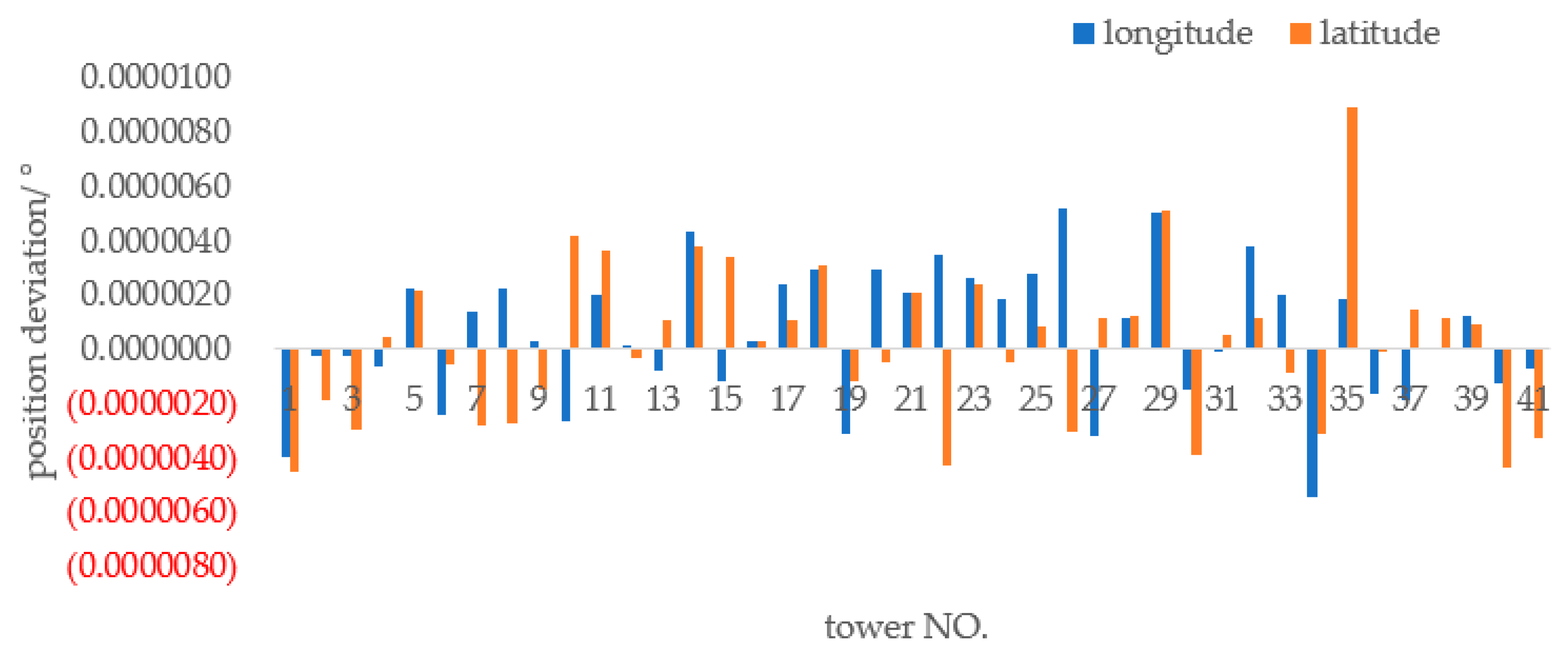
• The coordinates of the HV towers are localized accurately and robustly by extracting reliable center points of the cross-section layers in the height direction.

The proposed method automatically extracted and reconstructed transmission corridor objects (PLs and pylons) in the studied area using UAV Lidar data. It was efficient in terms of speed, quality, and scalability. The algorithm has a few requirements for the data, such as a moderate gap between points. When the data gap in the main direction of the PLs is bigger than 4 m, the results will be affected. The processing efficiency of the algorithm can be further improved, and other surrounding objects (buildings, trees, railways, other poles, etc.) and small components (nests) may be also extracted in the future. In addition, physical analysis for structural health monitoring will be investigated [74], taking the stability of the ground base into consideration, such as to detect the inclination or collapse of towers, etc. This could be further integrated via structure from motion (SfM) [75].

References

1. Ituen, I.; Sohn, G. The way forward: Advances in maintaining right-of-way of transmission lines. Geomatica 2010, 64, 451–462. [Google Scholar]
2. Chen, C.; Yang, B.; Song, S.; Peng, X.; Huang, R. Automatic clearance anomaly detection for transmission line corridors utilizing uav-borne lidar data. Remote Sens. 2018, 10, 613. [Google Scholar] [CrossRef]
3. Matikainen, L.; Lehtomäki, M.; Ahokas, E.; Hyyppä, J.; Karjalainen, M.; Jaakkola, A.; Kukko, A.; Heinonen, T. Remote sensing methods for power line corridor surveys. ISPRS J. Photogramm. Remote Sens. 2016, 119, 10–31. [Google Scholar] [CrossRef] [Green Version]
4. Cai, J.; Walker, R. Height estimation from monocular image sequences using dynamic programming with explicit occlusions. IET Comput. 2010, 4, 149–161. [Google Scholar] [CrossRef]
5. Yu, X.; Hyyppä, J.; Karjalainen, M.; Nurminen, K.; Karila, K.; Vastaranta, M.; Honkavaara, E. Comparison of Laser and Stereo Optical, SAR and InSAR Point Clouds from Air-and Space-Borne Sources in the Retrieval of Forest Inventory Attributes. Remote Sens. 2015, 7, 15933–15954. [Google Scholar] [CrossRef]
6. Vosselman, G.; Gorte, B.G.; Rabbani Shah, T.; Rabbani, T.; Sithole, G. Recognising structure in laser scanner point clouds. Int. Arch. Photogramm. Remote Sens. Spat. Inf. Sci. 2008, 46, 33–38. [Google Scholar]
7. Yang, B.; Dong, Z.; Liang, F.; Liu, Y. Automatic registration of large-scale urban scene point clouds based on semantic feature points. ISPRS J. Photogramm. Remote Sens. 2016, 113, 43–58. [Google Scholar] [CrossRef]
8. Wehr, A.; Lohr, U. Airborne laser scanning—An introduction and overview. ISPRS J. Photogramm. Remote Sens. 1999, 54, 68–82. [Google Scholar] [CrossRef]
9. Liu, H.; Chen, W.; Gao, X.-H. Analysis of vegetation-related failures on transmission lines from the view point of black outs. Power Syst. Technol. 2007, 31, 67–69. [Google Scholar]
10. Böhler, W. Comparison of 3D laser scanning and other 3D measurement techniques. In Recording, Modeling, and Visualization of Cultural Heritage; Taylor & Francis Group: London, UK, 2006; pp. 89–99. [Google Scholar]
11. Zeybek, M.; Şanlıoğlu, İ. Point cloud filtering on UAV based point cloud. Measurement 2019, 133, 99–111. [Google Scholar] [CrossRef]
12. Colomina, I.; Molina, P. Unmanned aerial systems for photogrammetry and remote sensing: A review. ISPRS J. Photogramm. Remote Sens. 2014, 92, 79–97. [Google Scholar] [CrossRef] [Green Version]
13. Pfeifer, N.; Mandlburger, G.; Otepka, J.; Karel, W. OPALS—A framework for Airborne Laser Scanning data analysis. Comput. Environ. Urban Syst. 2014, 45, 125–136. [Google Scholar] [CrossRef]
14. Toth, C.; Jóźków, G. Remote sensing platforms and sensors: A survey. ISPRS J. Photogramm. Remote Sens. 2016, 115, 22–36. [Google Scholar] [CrossRef]
15. Mills, S.J.; Castro, M.P.G.; Li, Z.; Cai, J.; Hayward, R.; Mejias, L.; Walker, R.A. Evaluation of aerial remote sensing techniques for vegetation management in power-line corridors. IEEE Trans. Geosci. Remote Sens. 2010, 48, 3379–3390. [Google Scholar] [CrossRef]
16. Qin, X.; Wu, G.; Lei, J. Detecting Inspection Objects of Power Line from Cable Inspection Robot. Sensor 2018, 18, 1284. [Google Scholar] [CrossRef] [PubMed]
17. Frank, M.; Pan, Z.; Raber, B.; Lenart, C. Vegetation management of utility corridors using high-resolution hyperspectral imaging and LiDAR. In Proceedings of the 2010 2nd Workshop on Hyperspectral Image and Signal Processing: Evolution in Remote Sensing (WHISPERS), Reykjavik, Iceland, 14–16 June 2010; p. 4. [Google Scholar]
18. Li, Z.; Bruggemann, T.S.; Ford, J.J.; Mejias, L.; Liu, Y. Toward automated power line corridor monitoring using advanced aircraft control and multisource feature fusion. J. Field Robot. 2012, 29, 4–24. [Google Scholar] [CrossRef]
19. Ahmad, J.; Malik, A.S.; Xia, L. Vegetation monitoring for high-voltage transmission line corridors using satellite stereo images. In Proceedings of the 2011 National Postgraduate Conference (NPC), Kuala Lumpur, Malaysia, 19–20 September 2011; IEEE: Piscataway, NJ, USA, 2011; pp. 1–5. [Google Scholar]
20. Ahmad, J.; Malik, A.S.; Xia, L.; Ashikin, N. Vegetation encroachment monitoring for transmission lines right-of-ways: A survey. Electr. Power Syst. Res. 2013, 95, 339–352. [Google Scholar] [CrossRef]
21. Ortega, S.; Trujillo, A.; Santana, J.M.; Suárez, J.P.; Santana, J. Characterization and modeling of power line corridor elements from LiDAR point clouds. ISPRS J. Photogramm. Remote Sens. 2019, 152, 24–33. [Google Scholar] [CrossRef]
22. Zhu, L.; Hyyppä, J. Fully-Automated Power Line Extraction from Airborne Laser Scanning Point Clouds in Forest Areas. Remote Sens. 2014, 6, 11267–11282. [Google Scholar] [CrossRef] [Green Version]
23. Grigillo, D.; Ozvaldič, S.; Vrečko, A.; Kosmatin Fras, M. Extraction of Power Lines from Airborne and Terrestrial Laser Scanning Data Using the Hough Transform. Geod. Vestn. 2015, 59, 246–261. [Google Scholar] [CrossRef]
24. Wang, Y.; Chen, Q.; Liu, L.; Li, K. A Hierarchical unsupervised method for power line classification from airborne LiDAR data. Int. J. Digit. Earth 2018, 1–17. [Google Scholar] [CrossRef]
25. Cheng, L.; Tong, L.; Wang, Y.; Li, M. Extraction of Urban Power Lines from Vehicle-Borne LiDAR Data. Remote Sens. 2014, 6, 3302–3320. [Google Scholar] [CrossRef] [Green Version]
26. Husain, A.; Vaishya, R.C. An Automated Method for Power Line Points Detection from Terrestrial LiDAR Data. In Emerging Technologies in Data Mining and Information Security; Springer: Singapore, 2019; pp. 459–472. [Google Scholar]
27. Melzer, T.; Briese, C. Extraction and Modeling of Power Lines from ALS Point Clouds. In Proceedings of the 28th Workshop of the Austrian Association for Pattern Recognition, Hagenberg, Austria, 17–18 June 2004. [Google Scholar]
28. Mclaughlin, R.A. Extracting transmission lines from airborne LIDAR data. IEEE Geosci. Remote Sens. Lett. 2006, 3, 222–226. [Google Scholar] [CrossRef]
29. Ritter, M.; Benger, W. Reconstructing Power Cables from LIDAR Data Using Eigenvector Streamlines of the Point Distribution Tensor Field. In Proceedings of the WSCG2012—20th International Conference in Central Europe on Computer Graphics, Visualization and Computer Vision, Plzen, Czech Republic, 25–28 June 2012. [Google Scholar]
30. Jwa, Y.; Sohn, G. A Piecewise Catenary Curve Model Growing for 3D Power Line Reconstruction. Photogramm. Eng. Remote Sens. 2012, 78, 1227–1240. [Google Scholar] [CrossRef]
31. Sohn, G.; Jwa, Y.; Kim, H.B. Automatic power line scene classification and reconstruction using airborne lidar data. ISPRS Ann. Photogramm. Remote Sens. Spat. Inf. Sci. 2012, 1, 167–172. [Google Scholar] [CrossRef]
32. Liu, Y.; Shi, J.; Liu, Z.; Huang, J.; Zhou, T. Two-Layer Routing for High-Voltage Powerline Inspection by Cooperated Ground Vehicle and Drone. Energies 2019, 12, 1385. [Google Scholar] [CrossRef]
33. Song, B.; Li, X. Power line detection from optical images. Neurocomputing 2014, 129, 350–361. [Google Scholar] [CrossRef]
34. Fryskowska, A. Improvement of 3D Power Line Extraction from Multiple Low-Cost UAV Imagery Using Wavelet Analysis. Sensors 2019, 19, 700. [Google Scholar] [CrossRef]
35. Jaw, Y.; Sohn, G. Wind adaptive modeling of transmission lines using minimum description length. ISPRS J. Photogramm. Remote Sens. 2017, 125, 193–206. [Google Scholar] [CrossRef]
36. Liu, Y.; Mejias, L. Real-time power line extraction from Unmanned Aerial System video images. In Proceedings of the 2012 2nd International Conference on Applied Robotics for the Power Industry, Zurich, Switzerland, 11–13 September 2012; IEEE: Piscataway, NJ, USA, 2013; pp. 52–57. [Google Scholar]
37. Arastounia, M.; Lichti, D.D. Automatic object extraction from electrical substation point clouds. Remote Sens. 2015, 7, 15605–15629. [Google Scholar] [CrossRef]
38. Nasseri, M.H.; Moradi, H.; Nasiri, S.M.; Hosseini, R. Power Line Detection and Tracking Using Hough Transform and Particle Filter. In Proceedings of the 2018 6th RSI International Conference on Robotics and Mechatronics, Tehran, Iran, 23–25 October 2018; pp. 130–134. [Google Scholar]
39. Liu, Z.; Liang, J.; Zhang, J. Power lines extraction from airborne lidar data using spatial domain segmentation. J. Remote Sens. 2014, 18, 61–76. [Google Scholar]
40. Jwa, Y.; Sohn, G. A multi-level span analysis for improving 3D power-line reconstruction performance using airborne laser scanning data. Int. Arch. Photogramm. Remote Sens. Spat. Inf. Sci. 2010, 38, 97–102. [Google Scholar]
41. Kim, H.B.; Sohn, G. Random forests based multiple classifier system for power-line scene classification. Int. Arch. Photogramm. Remote Sens. 2011, 5, 253–258. [Google Scholar] [CrossRef]
42. Guo, B.; Huang, X.; Zhang, F.; Sohn, G. Classification of airborne laser scanning data using JointBoost. ISPRS J. Photogramm. Remote Sens. 2015, 100, 71–83. [Google Scholar] [CrossRef]
43. Zhou, R.; Jiang, W.; Jiang, S. A Novel Method for High-Voltage Bundle Conductor Reconstruction from Airborne LiDAR Data. Remote Sens. 2018, 10, 2051. [Google Scholar] [CrossRef]
44. Araar, O.; Aouf, N.; Dietz, J.L.V. Power pylon detection and monocular depth estimation from inspection uavs. Ind. Robot-Int. J. 2015, 42, 200–213. [Google Scholar] [CrossRef]
45. Tilawat, J.; Theera-Umpon, N.; Auephanwiriyakul, S. Automatic detection of electricity pylons in aerial video sequences. In Proceedings of the 2010 International Conference on Electronics and Information Engineering, Kyoto, Japan, 1–3 August 2010; Volume 1, pp. 342–346. [Google Scholar]
46. Awrangjeb, M.; Islam, M.K. Classifier-free detection of power line pylons from point cloud data. ISPRS Ann. Photogramm. Remote Sens. Spat. Inf. Sci. 2017, 4, 81–87. [Google Scholar] [CrossRef]
47. Ortega, S.; Trujillo, A.; Santana, J.M.; Suárez, J.P. An image-based method to classify power line scenes in LiDAR point clouds. In Proceedings of the 12th International Symposium on Tools and Methods of Competitive Engineering, Las Palmas de Gran Canarias, Spain, 7–11 May 2018; pp. 585–593. [Google Scholar]
48. Li, Q.; Chen, Z.; Hu, Q. A model-driven approach for 3D modeling of pylon from airborne LiDAR data. Remote Sens. 2015, 7, 11501–11524. [Google Scholar] [CrossRef]
49. Guo, B.; Huang, X.; Li, Q.; Zhang, F.; Zhu, J.; Wang, C. A stochastic geometry method for pylon reconstruction from airborne lidar data. Remote Sens. 2016, 8, 243. [Google Scholar] [CrossRef]
50. Zhou, R.; Jiang, W.; Huang, W.; Xu, B.; Jiang, S. A Heuristic Method for Power Pylon Reconstruction from Airborne LiDAR Data. Remote Sens. 2017, 9, 1172. [Google Scholar] [CrossRef]
51. Lin, X.; Zhang, J. 3d power line reconstruction from airborne lidar point cloud of overhead electric power transmission corridors. Acta Geod. Cartogr. Sin. 2016, 45, 347–353. [Google Scholar]
52. Axelsson, P. Processing of laser scanner data—Algorithms and applications. ISPRS J. Photogramm. Remote Sens. 1999, 54, 138–147. [Google Scholar] [CrossRef]
53. Liang, J.; Zhang, J.; Deng, K.; Liu, Z. A New Power-Line Extraction Method Based on Airborne LiDAR Point Cloud Data. In Proceedings of the 2011 International Symposium on Image and Data Fusion, Tengchong, China, 9–11 August 2011; pp. 1–4. [Google Scholar]
54. Yin, H.Z.; Sun, X.; Nie, Z.G. An automated extraction algorithm of power lines based on airborne laser scanning data. Geogr. Geo-Inf. Sci. 2012, 28, 30–31. [Google Scholar]
55. Lefebvre, S.; Hoppe, H. Perfect spatial hashing. ACM Trans. Graph. 2006, 25, 579–588. [Google Scholar] [CrossRef]
56. Bastos, T.; Celes, W. GPU-accelerated Adaptively Sampled Distance Fields. In Proceedings of the 2008 IEEE International Conference on Shape Modeling and Applications, Stony Brook, NY, USA, 4–6 June 2008; pp. 171–178. [Google Scholar]
57. Brain, M.D.; Tharp, A.L. Perfect hashing using sparse matrix packing. Inf. Syst. 1990, 15, 281–290. [Google Scholar] [CrossRef]
58. Eitz, M.; Gu, L. Hierarchical Spatial Hashing for Real-time Collision Detection. In Proceedings of the IEEE International Conference on Shape Modeling and Applications 2007, Lyon, France, 13–15 June 2007; pp. 61–70. [Google Scholar]
59. Alcantara, D.A.; Sharf, A.; Abbasinejad, F.; Sengupta, S.; Mitzenmacher, M.; Owens, J.D.; Amenta, N. Real-time parallel hashing on the GPU. ACM Trans. Graphics (TOG) 2009, 28, 154. [Google Scholar] [CrossRef]
60. Pan, J.; Manocha, D. Fast GPU-based locality sensitive hashing for k-nearest neighbor computation. In Proceedings of the 19th ACM SIGSPATIAL International Conference on Advances in Geographic Information Systems, Chicago, IL, USA, 1–4 November 2011; pp. 211–220. [Google Scholar]
61. García, I.; Lefebvre, S.; Hornus, S.; Lasram, A. Coherent parallel hashing. ACM Trans. Graph. 2011, 30, 161. [Google Scholar] [CrossRef]
62. Koivisto, T.; Roman, T.; Enescu, M. Spatial Hashing for Enhanced Control Channel Search Spaces. U.S. Patent Application 13/224,825, 7 March 2013. [Google Scholar]
63. Duan, W.; Luo, J.; Ni, G.; Tang, B.; Hu, Q.; Gao, Y. Exclusive grouped spatial hashing. Comput. Graph. 2017, 70. [Google Scholar] [CrossRef]
64. Patel, P.; Garg, D. Perfect Hashing Base R-tree for multiple queries. In Proceedings of the 2014 IEEE International Advance Computing Conference (IACC), Gurgaon, India, 21–22 February 2014; pp. 636–640. [Google Scholar]
65. Nießner, M.; Zollhöfer, M.; Izadi, S.; Stamminger, M. Real-time 3D reconstruction at scale using voxel hashing. ACM Trans. Graph. 2013, 32, 169. [Google Scholar] [CrossRef]
66. Weinmann, M.; Urban, S.; Hinz, S.; Jutzi, B.; Mallet, C. Distinctive 2d and 3D features for automated large-scale scene analysis in urban areas. Comput. Graph. 2015, 49, 47–57. [Google Scholar] [CrossRef]
67. Guan, H.; Yu, Y.; Li, J.; Ji, Z.; Zhang, Q. Extraction of power-transmission lines from vehicle-borne lidar data. Int. J. Remote Sens. 2016, 37, 229–247. [Google Scholar] [CrossRef]
68. Kim, H.B.; Sohn, G. 3D classification of power-line scene from airborne laser scanning data using random forests. Int. Arch. Photogramm. Remote Sens. 2010, 38, 126–132. [Google Scholar]
69. Jwa, Y.; Sohn, G.; Kim, H.B. Automatic 3D powerline reconstruction using airborne lidar data. Int. Arch. Photogramm. Remote Sens. 2009, 38, 105–110. [Google Scholar]
70. Lai, X.; Dai, D.; Min, Z.; Yong, D.U. Powerline three-dimensional reconstruction for lidar point cloud data. J. Remote Sens. 2014, 18, 1223–1229. [Google Scholar]
71. Arastounia, M.; Lichti, D.D. Automatic extraction of insulators from 3D LiDAR data of an electrical substation. ISPRS Ann. Photogramm. Remote Sens. Spat. Inf. Sci. 2013, 2, 19–24. [Google Scholar] [CrossRef]
72. Chen, C.; Rao, Z.; Yang, B.; Mai, X.; Wang, K. Safety inspection and intelligent diagnosis of transmission line based on unmanned helicopter of multi sensor data acquisition. High Volt. Eng. 2015, 41, 159–166. [Google Scholar]
73. Xie, X.; Peng, X.; Liu, Z.; Mai, X.; Zuo, Z.; Wang, K. Unmanned helicopter route planning and optimization for power line inspection. Sci. Surv. Mapp. 2015, 40, 87–91. [Google Scholar]
74. Vacca, G.; Mistretta, F.; Stochino, F.; Dessi, A. Terrestrial Laser Scanner for monitoring the deformations and the damages of buildings. Int. Arch. Photogramm. Remote Sens. Spat. Inf. Sci. 2016, XLI-B5, 453–460. [Google Scholar] [CrossRef]
75. Fausto, M.; Giannina, S.; Flavio, S.; Giuseppina, V. Structure from Motion Point Clouds for Structural Monitoring. Remote Sens. 2019, 11, 1940. [Google Scholar] [Green Version]
Figure 1. The workflow of transmission power line and pylon extraction and reconstruction.
Remotesensing 11 02600 g001
Figure 2. Voxels colored by height: (a) voxel blocks including power lines (PLs); (b) voxel blocks including a pylon; (c) voxel blocks including no power transmission objects.
Remotesensing 11 02600 g002aRemotesensing 11 02600 g002b
Figure 3. Parts of the point cloud of transmission line from unmanned aerial vehicle (UAV) data (colored by height): (a) side view; (b) top view.
Remotesensing 11 02600 g003
Figure 4. Height distribution of points in a block of the transmission corridor: (a) height difference between PLs and other objects in the normalized data; (b) height histogram of the point cloud where the vertical axis is the number of points.
Remotesensing 11 02600 g004aRemotesensing 11 02600 g004b
Figure 5. PL extraction: (a) 3D grid clustering results of the data in Figure 3a (colored by individual cluster); (b) PL segments segmented by height distance (colored by height); (c) PL segments extracted by dimensional feature (colored by grids); (d) The clustering result of individual lines within a span (colored by individual line); (e) PL extraction based on local collinearity, and two examples of extracted PLs including both high-voltage (HV) and low-voltage PLs (colored by height).
Remotesensing 11 02600 g005
Figure 6. Illustration of the candidate HV tower extraction process: (a) the overall view of the data without PL points; (b) partial view of the towers in (a); (c) detailed view of a tower in (b); (d) a sub-dataset to be processed with PL points removed; (e) grids with big height differences; (f) results of grid clustering colored by height.
Remotesensing 11 02600 g006
Figure 7. The spatial relationship between PLs and towers.
Remotesensing 11 02600 g007
Figure 8. Refined extraction results of pylons and PLs: (a) preliminary results with cross-over PLs and isolated tall trees; (b) example of extracted PLs; (c) example of detected transmission towers; (d) the refined result within a span.
Remotesensing 11 02600 g008
Figure 9. 3D reconstruction of PLs in a span: (a) fitted PLs within a span; (b) fitted PLs with two adjacent pylons (rendering by electrical phase).
Remotesensing 11 02600 g009
Figure 10. A schematic diagram of HV tower: (a) drum-like tower; (b) goblet-like tower; (c) tower in a zigzag structure; (d) cat-head-like tower.
Remotesensing 11 02600 g010
Figure 11. Illustration of HV tower center localization: (a) The point cloud of an incomplete HV transmission tower; (b) Center points by layers; (c) The procedure of center point selection; (d) Identified center points.
Remotesensing 11 02600 g011
Figure 12. The pylon reconstruction: (a) pylon modeling; (b) the diagram for insulator searching; (c) the reconstruction of the labeled insulators.
Remotesensing 11 02600 g012
Figure 13. The experimental data and the large UAV inspection system: (a,b) Dataset 1 and Dataset 2 from Guangdong Province, respectively; (c) the rotor-wing UAV platform; (d) the laser scanner.
Remotesensing 11 02600 g013
Figure 14. PL extraction: (a) DSM after grid calculation; (b) local extraction of PL segments; (c) global extraction by grouping; (d) detailed result of PLs.
Remotesensing 11 02600 g014
Figure 15. Tower extraction: (a) schematic map of the original data without PLs; (b) the result of the big difference grid in Dataset 1; (c) grid clustering by height of the data in (b); (d) the refined results of the dataset in (b); (e) intermediate result of Dataset 2; (f) the refined results of Dataset 2.
Remotesensing 11 02600 g015aRemotesensing 11 02600 g015b
Figure 16. Refinement of the results: (a) the reduced tower point cloud; (b,c) the refined result of transmission elements in the cross-over area; (d) reconstructed transmission lines from Dataset 2; (e) reconstruction result within a span; (f) reconstruction result in Reference [69] (containing low-voltage PLs).
Remotesensing 11 02600 g016
Figure 17. Visualization of some of the center positions.
Remotesensing 11 02600 g017
Figure 18. The position deviation of the calculated center points of the HV towers in Dataset 1.
Remotesensing 11 02600 g018
Figure 19. Reconstruction of the transmission corridor: (a) reconstruction of PLs; (b) center points of extracted towers; (c) modeling of the 3D scene in view of the modeling center of pylons.
Remotesensing 11 02600 g019
Figure 20. Sketch map of the spatial hashing storage schema.
Remotesensing 11 02600 g020
Figure 21. Subdivision analysis of the power corridor data: (a) height histogram of the point cloud where the vertical axis is the number of points; (b) diagram of PL point distribution and the gap in vertical distribution; (c) a point cloud fragment containing PLs; (d) height histogram of points in the data within two spans.
Remotesensing 11 02600 g021
Figure 22. Height clustering in pylon segmentation: (a) grids of large height difference; (b) a close-up view of a tower; (c,d) removal of points adjacent to a pylon.
Remotesensing 11 02600 g022aRemotesensing 11 02600 g022b