Article

An Accurate Method to Distinguish Between Stationary Human and Dog Targets Under Through-Wall Condition Using UWB Radar

Department of Medical Electronics, School of Biomedical Engineering, Fourth Military Medical University, Xi’an 710032, China
*
Authors to whom correspondence should be addressed.
Remote Sens. 2019, 11(21), 2571; https://doi.org/10.3390/rs11212571
Submission received: 27 September 2019 / Revised: 25 October 2019 / Accepted: 30 October 2019 / Published: 1 November 2019
(This article belongs to the Special Issue Radar Remote Sensing on Life Activities)

Abstract

:
Research work on distinguishing humans from animals can help provide priority orders and optimize the distribution of resources in earthquake- or mining-related rescue missions. However, the existing solutions are few and their stability and accuracy of classification are less. This study proposes an accurate method for distinguishing stationary human targets from dog targets under through-wall condition based on ultra-wideband (UWB) radar. Eight humans and five beagles were used to collect 130 samples of through-wall signals using the UWB radar. Twelve corresponding features belonging to four categories were combined using the support vector machine (SVM) method. A recursive feature elimination (RFE) method determined an optimal feature subset from the twelve features to overcome overfitting and poor generalization. The results after ten-fold cross-validation showed that the area under the receiver operator characteristic (ROC) curve can reach 0.9993, which indicates that the two subjects can be distinguished under through-wall condition. The study also compared the ability of the proposed features of four categories when used independently in a classifier. Comparison results indicated that wavelet entropy-corresponding features among them have the best performance. The method and results are envisioned to be applied in various practical situations, such as post-disaster searching, hostage rescues, and intelligent homecare.

Graphical Abstract

1. Introduction

The rapid developments in ultra-wideband (UWB) radar technology [1,2,3,4,5,6,7] have attracted increasing interest in civilian and military applications, such as earthquake and hostage rescue operations and gesture recognitions. The technologies of radar imaging, localization, and action recognition have been significantly improved over the past decade, and several research groups are focusing on the distinction between humans and animals based on the advancements in radar technologies. The work in [8] developed a feature-based classification method for walking movements in animals versus humans for border security applications. The research in [9] proposed a classification algorithm using micro-Doppler signals obtained from humans and dogs moving in four different directions, and [10] combined the Gaussian mixture model and the hidden Markov model to distinguish between slow moving animal and human targets to detect potential livestock thieves and poachers within reserves and farmland.
However, these research works between humans and animals have concentrated on the moving states of humans and animals, and there have been no reports focusing on the distinction in stationary state and through-wall condition. There is an urgent need to distinguish between stationary humans and animals under through-wall conditions for post-disaster rescuing applications when trapped targets are buried and unable to move. This work will help optimize the distribution of rescue resources and boost the confidence of rescuers in earthquake search, thereby ensuring the safety of hostages by eliminating the impact of pet signals in anti-terrorist rescue operation in the presence of barriers such as walls. Therefore, distinction between stationary humans and other species under through-wall condition is a significant and to be further resolved research work.
UWB radar can detect the vital signs of human and animal targets based on their quasi-periodic respiration or non-periodic body movements. Considering that humans have more powerful psychological and mental control, the signs caused by the micro motions in humans are more regular than those in animals. The work in Otero, M. [11] found that the spectrum of radar echo signals is different between human targets and other detected slow-moving targets; however, it is mainly based on their different walking speed, implying that this method is not applicable in earthquake search and hostage rescue operations because the targets are generally stationary.
Dogs are most likely to appear where it is necessary to distinguish between humans and animals considering the actual situations. In Wang, Y. et al. [12], Wang extracted wavelet entropy and its standard deviation using signals of target position based on 400 MHz UWB radar. The results show that the two features have evident differences for human and dog targets. In [13], the classification accuracy of human target recognition can achieve 86% and the accuracy of dog target recognition can achieve 84% using wavelet entropy alone in through-wall conditions. When only standard deviation of wavelet entropy is utilized, the classification accuracy can achieve 86% for both human and dog targets. In her experiments, a total of ten humans and five dogs were used with five and ten times signal acquisitions per human and dog, respectively.
Meanwhile, Yu, X. et al. [14] and Yin, Y. et al. [15] proposed some other features, whose classification ability performs well when used independently in distinguishing humans from dogs, such as optimal correlation coefficient of micro vibration (OCCMV), standard deviation change rate of micro vibration (StdCRMV), energy ratio of the reference frequency band (ERRFB), etc. However, only one or two of the features above, at most, are combined together to achieve the classification objectives of human targets and dog targets each time in previous studies. Consequently, the robustness and classification accuracy are unguaranteed because of the individual differences, no matter whether for human targets or dog targets. For example, for some individual dogs, the values and ranges of OCCMV or StdCRMV can resemble those of human beings, so much so that it is almost impossible to distinguish between them when only one or two features are combined.
In this study, twelve feature species belonging to four categories are first extracted, including two energy-corresponding features, two correlation coefficient-corresponding features, four wavelet entropy-corresponding features, and four frequency-corresponding features. Then, a support vector machine (SVM)-based feature selection and classification strategy are utilized to choose an optimal feature subset. Finally, after 100 rounds of ten-fold cross-validation, a classifier with reliable generalization and stability is successfully modeled. Meanwhile, the value of the area under the curve (AUC) of the classifier also reaches the highest level, which is adopted to evaluate the overall performance of the classifier. Higher values of AUC indicate better classifier performance. Thus, the combination of these features improves the classification accuracy and enhances the stability of the proposed system in distinguishing between human and dog targets.
The paper is organized as follows. Section 2 introduces the working principles of the UWB radar and signal preprocessing. Section 3 describes the extraction of the abovementioned twelve features belonging to four categories. In Section 4, the classification procedure and feature selection strategy based on SVM are introduced. Experimental results are presented in Section 5. Section 6 discusses the significance and future research considerations. The work is concluded in Section 7.

2. UWB Radar System and Signal Preprocessing

2.1. UWB Radar System

The block diagram of the utilized UWB radar system is illustrated in Figure 1. Firstly, the pulse generator generated trigger pulses with a center frequency and pulse repetition frequency of 500 MHz and 128 KHz, respectively. Then, the pulses were sent to the transmitter to excite the transmitter antenna (TA), where they were shaped into bipolar pulse. Next, the bow-tie dipole antenna transmitted the vertically polarized pulses with peak power of approximately 5 W. Meanwhile, the trigger pulses were sent to the delay unit to produce a series of software-controlled range gates of 300 ps in width to turn on the receiver, which was identical with the transmitting one. Finally, through the receiving antenna (RA), return pulse only within the range gates were sampled, integrated, amplified, and then transferred to the computer for further analysis [16]. The detailed parameters of the UWB radar system are listed in Table 1.
After signal acquisition, the raw echo data D ( m , n ) are stored in the form of waveforms, where m = 1, 2, , M denotes the sampling point in propagation time, and n =1, 2, , N denotes the sampling point in observation time. The two-dimensional (2-D) pseudo-color image of raw echo data is illustrated in Figure 2, when the human target is 2.5 m behind the wall. The time-axis associated with range along each received waveform is termed as the “fast-time” and denoted by τ that is in the order of nanoseconds. The time-axis corresponding to the acquisition time of waveforms along the measurement duration is termed as “slow-time” and denoted by t that is in the order of seconds. Each waveform contains M = 2048 sample points and the recorded profile is τ m a x = 20 ns long, corresponding to a detection range of 3 m. The amplitudes along slow-time at each sample point, which stands for a specific range, are defined as point signal. The scanning speed is 64 waveforms per second which is higher than the Nyquist sampling rate for the respiration; thus, the number of recorded waveforms in slow-time can be written as N = 64 t .

2.2. Signal Preprocessing

Signal preprocessing steps, including distance accumulation, normalization along the fast-time dimension, direct current (DC) removal, 2 Hz low-pass (LP) filtering, and adaptive filtering based on least mean square (LMS) are first performed, as illustrated in Figure 3. It should be noted that all subsequent feature extractions are based on the preprocessed signals using the steps shown in Figure 3.
Distance accumulation will help reduce the computational complexity effectively on the premise of guaranteeing detailed information. It can be determined by:
D a t a A ( x , n ) = 1 Q m = Q ( x 1 ) + 1 Q x D ( m , n )
where D a t a A ( x , n ) is the echo matrix data after distance accumulation and Q is the distance window width along the fast-time dimension. The value of x is x = 1, 2, , X, and X denotes the distance point number on the fast-time dimension after accumulation.
Next, normalization along the fast-time dimension is accomplished to guarantee that the waveforms have the comparable amplitudes, and its processing is as follows:
D a t a N ( m , x ) = 2 × D a t a A ( m , x ) min 1 m M [ D a t a A ( m , x ) ] max 1 m M [ D a t a A ( m , x ) ] min 1 m M [ D a t a A ( m , x ) ] 1
DC removal will remove the DC component and baseline drift. The step of DC removal is given by:
D a t a D C ( x , n ) = D a t a N ( x , n ) 1 100 n = x x + 99 D a t a N ( x , n )
The cut-off frequency of the low-pass filter is chosen to be 2 Hz to filter out the high-frequency noise and retain respiratory signals. It can be determined by:
D a t a L P ( x , n ) = D a t a D C ( x , n ) × H ( t )
where H(t) is the impulse response function of the finite impulse response (FIR) filter [13].
Adaptive filtering by means of the least mean square (LMS) algorithm is used to suppress the strong clutters. It is illustrated and verified in [17].
Matrix data D a t a A F ( x , n ) is obtained after the execution of all preprocessing steps. The 2-D pseudo-color image of the preprocessed signal is shown in Figure 4, when the human target is 2.5 m behind the wall. The subsequent feature calculation will proceed with D a t a A F ( x , n ) .

3. Feature Extraction

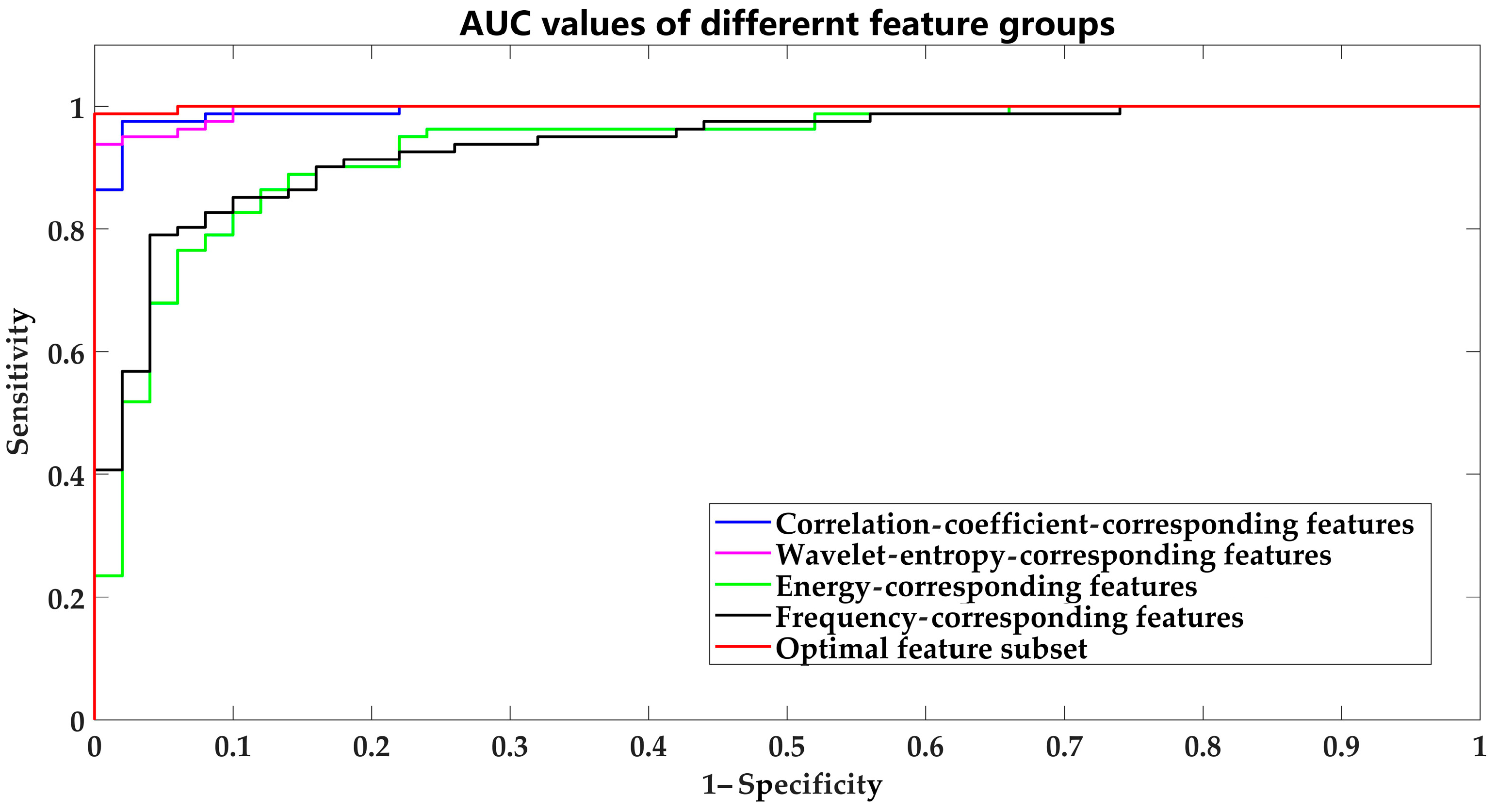
According to the accumulation of research results in recent years, 12 capable features belonging to four categories, consisting of two energy-corresponding features, two correlation coefficient-corresponding features, four wavelet entropy-corresponding features, and four frequency-corresponding features were utilized after signal preprocessing. The detailed feature descriptions are described below.

3.1. Energy-Corresponding Features

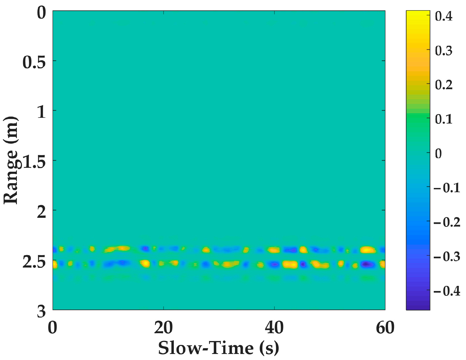
• Standard deviation change rate of micro vibration ( S t d C R M V )
When calculating S t d C R M V , Q = 1 . Preliminary researches have shown that the deviations in the amplitude values in target position are the greatest in D a t a A F ( x , n ) , indicating that the standard deviation ( S t d ) of the target signal is the greatest. Target signal is defined as the specific point signal which is right at the target position. The calculation of S t d is expressed as:
S t d = i = 1 n ( y i y ¯ ) 2 n 2
where y is a scalar denoting amplitudes of the point signals. Then, an optimal window (OW), where the target signal is in the middle position, is chosen along the fast-time dimension with fixed width, and the S t d of every point signal in the OW is calculated. Accordingly, the S t d C R M V is expressed as:
S t d C R M V = S t d m a x S t d m i n S t d m a x × 100 %
where S t d m a x is the max S t d value and S t d m i n is the min S t d value within the OW. According to the work in [
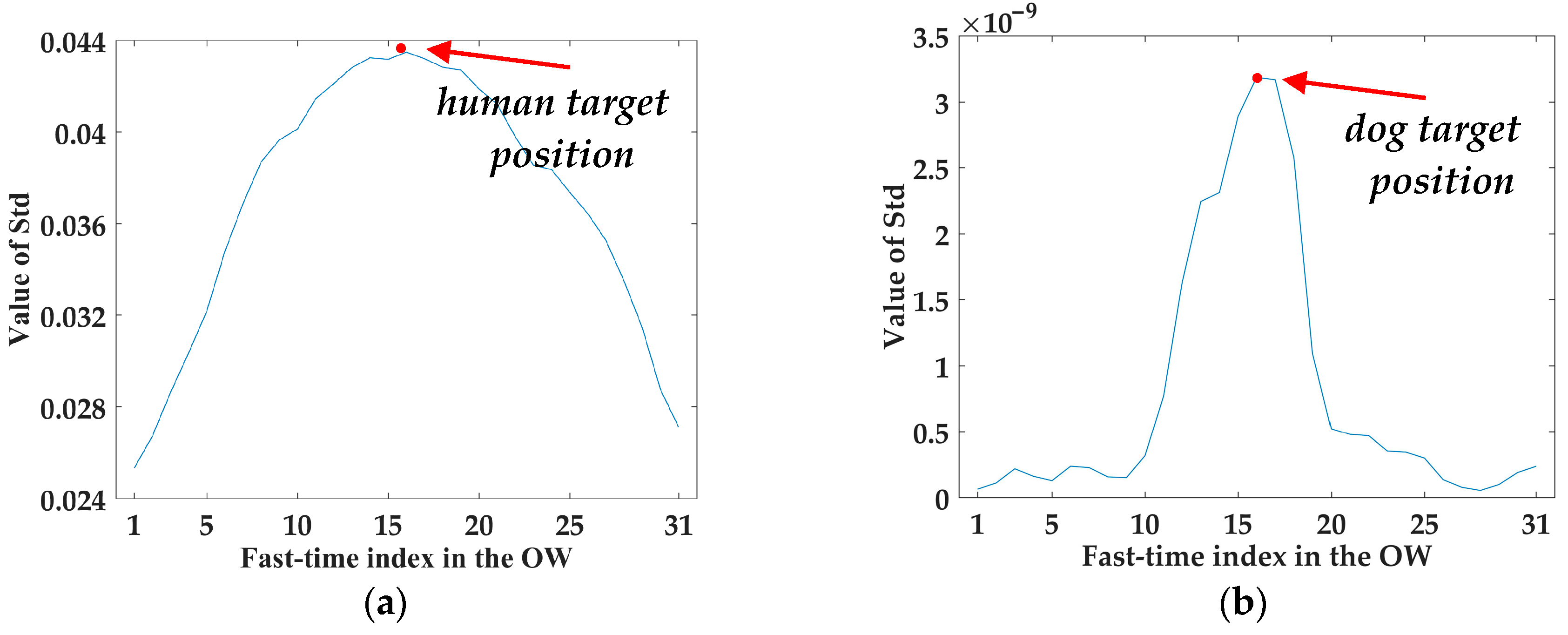
18], it is better to choose the width of the OW as o w S t d = 15 , so that the difference between human targets and dog targets will be largest. Figure 5 illustrates the value of S t d closer and further than the target’s position for 15 points of human and dog targets, respectively. Generally, the changing trend of S t d in the OW of human targets is much gentler than that of dog targets. Therefore, the S t d C R M V of human targets is much lower than that of dog targets.
• Energy ratio of the reference frequency band ( E R R F B )
In the calculation of E R R F B , the preprocessing steps are similar to that of S t d C R M V . The difference is that Q = 10 and the normalization is along the slow-time dimension, as illustrated in Equation (7). Thus, the 2048 points along the fast-time index associated to the range are compressed into 200 points [18].
D a t a N ( x , n ) = 2 × D a t a A ( x , n ) min 1 n N [ D a t a A ( x , n ) ] max 1 n N [ D a t a A ( x , n ) ] min 1 n N [ D a t a A ( x , n ) ] 1
Then, ensemble empirical mode decomposition (EEMD) is performed on the target signal. EEMD is a noise-eliminating algorithm, and it can decompose the original target signal into a series of intrinsic mode function (IMF) components with different characteristic scales by adding multiple sets of different white noises [19,20,21]. Its procedures are as follows:
  • Add a random white noise signal w n j ( t ) to the original target signal S i g n a l o (t):
    S i g n a l j ( t ) = S i g n a l o ( t ) + w n j ( t )
    where S i g n a l j ( t ) is the noise-added signal, j = 1, 2, …, TN and TN is the number of trails, which is chosen to be 50 here.
  • Decompose S i g n a l j ( t ) into a series of IMF components I M F i , j as follows:
    S i g n a l j ( t ) = i = 1 V j I M F i , j + R e s i d u e j
    where I M F i , j is the i-order IMF component of the j-th trail, V j is the number of IMF components of the j-th trail, and R e s i d u e j is the residue of the j-th trail.
  • If j < TN, then steps 1 and 2 are repeated, and different random white noise signals are added each time.
  • Obtain V = min ( V 1 , V 2 , ,   V T N ) and calculate the ensemble average of corresponding IMF components of the decompositions as the EEMD result:
    I M F i = 1 T N j = 1 T N I M F i , j
    where i = 1, 2, …, V . I M F i is the ensemble average of corresponding IMF components of the decompositions.
After dividing the original target signal into V-order IMF components by EEMD, noise will be eliminated using the discriminant method as expressed in Equations (11) and (12):
β ( i ) = { 0          i = 1 1 i 1 j = 1 i 1 η ( j ) η ( i ) η ( i )          i = 2 , 3 , , V
η ( i ) = n 1 n 2 R I M F i 2 ( n ) R I M F i 2 ( n )         i = 2 , 3 , , V
where β is the energy concentration ratio and R I M F i is the discrete autocorrelation sequence of the i-order (i = 2,3, …,V) IMF components of the target signal, which is defined in Equation (10). [ n 1 , n 2 ] denotes the interval with length of three points wherein the symmetric point of R I M F i is in the middle and η denotes energy concentration ratio in the interval. When the decline rate of energy concentration ratio β ( v ) satisfies the condition β ( v ) > 2 , the v -order IMF component is considered as denoised signal. The reconstructed signal s r e is expressed in Equation (13).
s r e = i = v V I M F i
E R R F B is the energy proportion of the reconstructed signal in human respiratory frequency band (0.2–0.4 Hz), expressed in Equation (14).
E R R F B = E r e _ h b E r e × 100 %
where E r e is the total energy of the reconstructed signal in frequency domain, and E r e _ h b is the energy of reconstructed signal in the reference frequency band, i.e., the human respiratory frequency band. Generally, E R R F B of humans is approximately 40% and that of dogs is approximately 18% [15,19].

3.2. Correlation Coefficient-Corresponding Features

• Optimal Correlation Coefficient of Micro vibration ( O C C M V )
Because the details are particularly important in calculation with O C C M V , the distance window width here is Q = 1 , and the width of OW here is o w O C C M V = 15. In this way, O C C M V is expressed as Equations (15) and (16):
C C M V ( y ) = i = 1 N ( T S i T S ¯ ) ( Y i Y ¯ ) i = 1 N ( T S i T S ¯ ) 2 i = 1 N ( Y i Y ¯ ) 2
O C C M V = y = 1 2 × o w O C C M V + 1 C C M V ( y ) 2 × o w O C C M V + 1
where TS represents the amplitudes of target signal, and Y the amplitudes of other point signals within the OW. The horizontal bar above the TS and Y denotes the calculation of the average value. C C M V ( y ) 
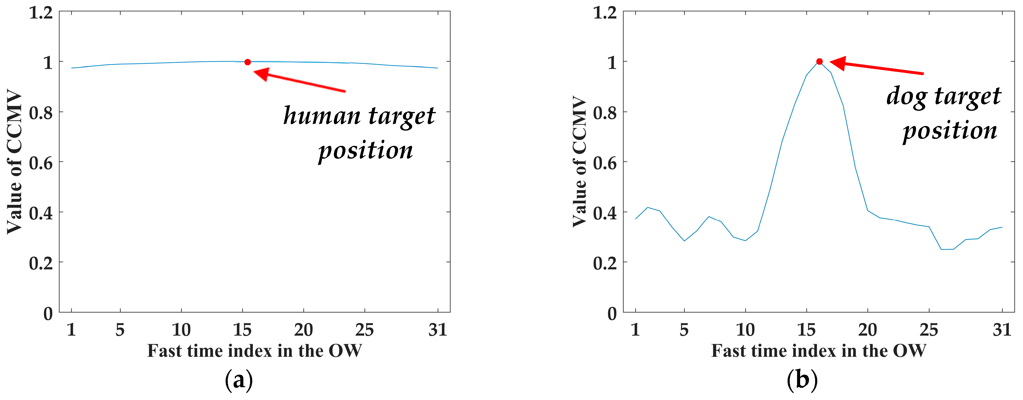
is the correlation coefficient between target signal and another point signal in the OW. O C C M V is the mean value of the C C M V of each point signal in the OW. Generally, the C C M V of human targets is very stable in the OW, close to one. Whereas the change of C C M V of dog targets is greater. So the O C C M V of human targets is larger than that of dog targets. The comparison result of C C M V of human targets and dog targets is expressed as in Figure 6.
• Change rate of correlation coefficient of micro vibration ( C R C C M V )
As illustrated in Figure 6, the trend of change of human target is stable, whereas the trend of change of dog target is more intense. Therefore, the C R C C M V of human targets is much smaller than that of dog targets. Equation (17) defines the calculation of C R C C M V .
C R C C M V = C C M V m a x C C M V m i n C C M V m a x × 100 %

3.3. Wavelet Entropy-Corresponding Features

In the calculation of wavelet entropy-corresponding features, the parameter of Q in the preprocessing steps is chosen to be Q = 10 and the normalization is along slow-time dimension. Thus, the raw echo data are compressed into 200 points along the fast-time index, similar to the preprocessing of E R R F B .
• Mean of wavelet entropy of target signal ( M W E )
Wavelet analysis can provide optimal time-frequency resolution of the signal and entropy can quantify the signal’s frequency patterns as a relevant measure of order or disorder in a dynamic system. Wavelet entropy (WE) combines the advantages of both. It can accurately characterize the dynamic change information of time-frequency variation of non-stationary signal complexity in time domain. More signal components indicate a more complex and irregular signal, and a larger value of wavelet entropy. Generally, dog signals are more complex than human signals [12,22]. Therefore, the M W E of human targets is much smaller than that of dog targets.
In the calculation of M W E , wavelet transform is first performed, followed by the calculation of relative wavelet energy. In Matsui, T. et al. [23], Morlet first considered wavelets as a family of functions generated by translations and dilations of a unique function called the “mother wavelet” ψ ( t ) . The family wavelet is expressed as:
ψ a , b ( t ) = | a | 1 2 ψ ( t b a )                 a ,   b   R ,    a 0
where a is the scaling parameter which measures the degree of compression, b is the translation parameter which determines the time location of the wavelet, and t represents time. Let L 2 ( ) be the real square integrable function space, the discrete wavelet transform of a signal S ( t )   L 2 ( ) is defined as [12,13]:
C j ( k ) = + S ( t ) ψ j , k ( t ) d t
where C j ( k ) is wavelet coefficient of wavelet sequence. For practical signal processing, the signal is assumed to be given by the sampled values S = { s 0 ( n ) ,   n = 1 , , N } . Then, the signal reconstructed by wavelet transform is expressed as:
S ( t ) = j = J 1 k C j ( k ) ψ j , k ( t ) = j = J 1 r j ( t )
where ψ j , k ( t ) = 2 j 2   ψ ( 2 j t k ) with j, k ∈ Z, and ψ ( t ) is the mother wavelet. j = 1 , 2 ,   ,   J is the number of resolution levels and its maximum value is J = log 2 N if the decomposition is performed over all resolution levels. k is the time index and r j ( t ) is the residual at scale j.
In radar signal processing, the signal is divided among non-overlapping temporal windows of length L , and the length is chosen to be L = 128 empirically. Then, appropriate signal values are assigned to the central point of the time window for each interval i = 1 ,   2 ,   ,   N T ,      N T , = N / L . Next, by considering the mean wavelet energy instead of the total wavelet energy, the mean energy at each resolution level j for the time window i using the wavelet coefficient is:
E j ( i ) = 1 N j k = ( i 1 ) L + 1 i · L | C j ( k ) | 2
where N j is the number of wavelet coefficients at resolution j involved in the time widow i . Then, the total energy of wavelet coefficient at interval i is expressed as:
E t o t a l ( i ) = j < 0 E j ( i )
Next, the relative wavelet energy that represents the energy’s probability distribution in scales is obtained by:
p j ( i ) = E j ( i ) / E t o t a l ( i )
Finally, the average wavelet entropy of the whole time period is given by:
M W E = 1 N T i = 1 N T ( j < 0 p j ( i ) · ln [ p j ( i ) ] )
• Standard deviation of wavelet entropy of target signal ( S t d W E )
S t d W E is a feature to quantitatively describe the fluctuation degree of wavelet entropy. S t d W E of human targets is much smaller than that of dog targets, since human target signals are more regular [12,13], generally speaking. It is given by:
S t d W E = { 1 N T i = 1 N T ( j < 0 p j ( i ) · ln [ p j ( i ) ] M W E ) 2 } 1 2
• Mean of MWE in the OW window ( M M W E O W )
In the calculation of M M W E O W , an OW, where the target point signal is right in the middle, is also needed and the width is chosen to be o w M M W E = 20 . M M W E O W is the mean value of MWE of each point signal closer and further the target position for o w M M W E point, i.e., the mean value of MWE in the OW. It is given by:
M M W E O W = 1 2 o w M M W E + 1 i = P o w M M W E P + o w M M W E M W E ( i )
where P is the position of target point signal.
• Ratio of wavelet entropy ( R W E )
R W E is the ratio of the mean value of M W E inside and outside the OW. It is expressed as:
M M W E o o w = 1 N 2 o w M M W E 1 i = 1 , i ( P o w M M W E ) : ( P + o w M M W E ) N M W E ( i )
R W E = M M W E O W M M W E o o w

3.4. Frequency-Corresponding Features

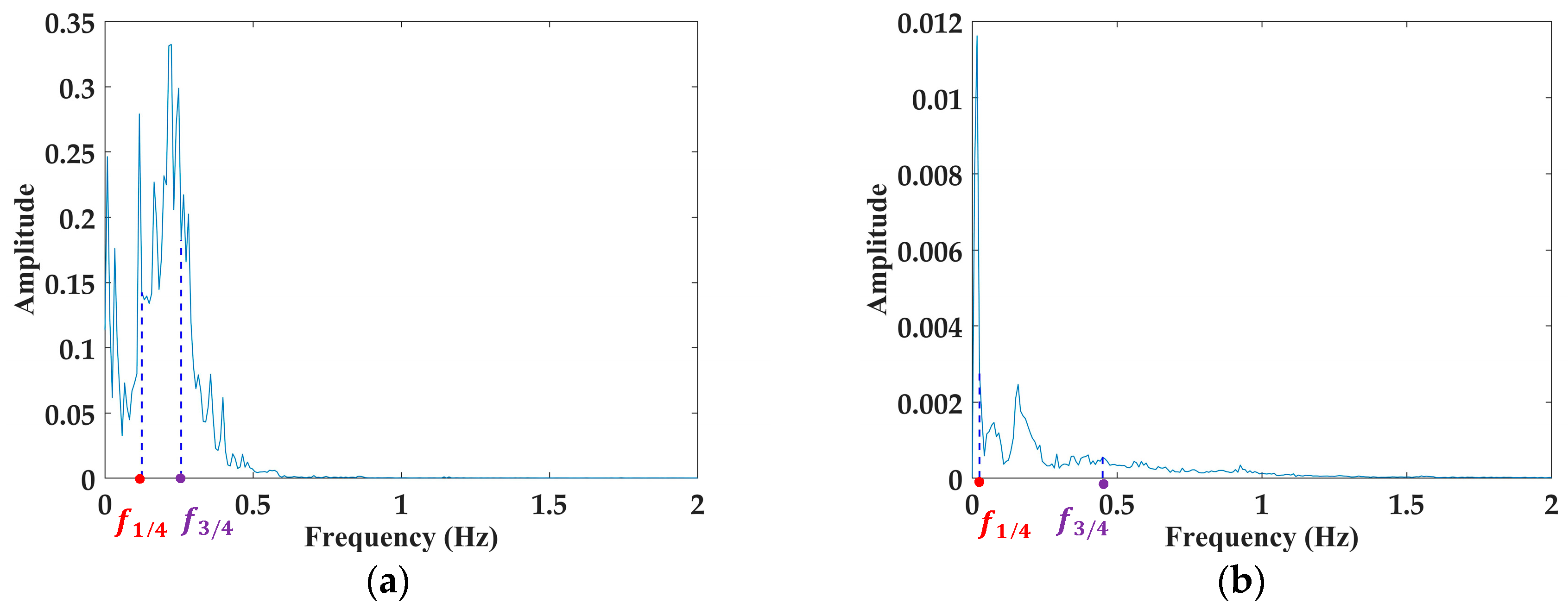
In this section, according to the research and accumulation of our group, it was found that the spectrum distribution of human targets in Hilbert marginal spectrum is different from that of dog targets. The curve of Hilbert marginal spectrum of human targets steeps slightly and the shape of the area under the curve is narrow and high. In contrast, the curve of dog targets is slightly gentle and the shape of the area under the curve is wide and low. Therefore, the frequency value corresponding to 1/4 total frequency band area, 3/4 total frequency band area under the Hilbert marginal spectrum curve, and the width between the above two are extracted.
•  f 1 / 4 ,   f 3 / 4 and width between   f 1 / 4 and f 3 / 4 ( W O H M S )
In this step, EEMD is performed first to process the target signal as Equations (8)–(13) illustrate. Then, Hilbert transformation is implemented in each IMF component of the reconstructed signal s r e .
I M F ^ i ( t ) = 1 π I M F i ( τ ) t τ d τ
Next, the analytical signals are constructed by:
z i ( t ) = I M F i ( t ) + j   I M F ^ i ( t ) = α i ( t ) e j φ i ( t )
The amplitude of the analytical signals is expressed by α i ( t ) = I M F i ( t ) 2 + I M F ^ i ( t ) 2 and the instantaneous phase is expressed as φ i ( t ) = arctan [ I M F ^ i ( t ) I M F i ( t ) ] . Then, the Hilbert marginal spectrum can be given by:
h ( ω ) = 0 T ( R e i = 1 V u s e f u l α i ( t ) e j ( d t d φ i ( t ) ) d t ) d t
where T is the total signal duration and V u s e f u l is the total IMF component number of the reconstructed signals. ω is the instantaneous frequency which is defined as ω = 2 π d φ i ( t ) d t [24]. The comparison results of Hilbert marginal spectrum of human targets and dog targets are demonstrated in Figure 7.
The f 1 / 4 and f 3 / 4 are the frequency values of the points corresponding to 1/4 total frequency band area and 3/4 total frequency band area, respectively, in Figure 7. Accordingly, W O H M S is given by:
W O H M S = f 3 / 4 f 1 / 4
• Respiratory Frequency ( R F )
After performing Fourier transform of the target signal, the R F of human targets and dog targets can be obtained.

4. SVM-Based Classification Procedure and Feature Selection Strategy

A support vector machine (SVM) is a type of generalized linear classifier which classifies data by supervised learning. Its decision boundary is the maximum margin hyperplane for learning samples. SVM classifier is chosen here because it has good performance for small samples when dividing data into two categories, which fits well with our purpose of distinguishing human beings from dogs.
Although the 12 features are calculated for each sample, these features may not contribute equally to improving the ability of distinguishing human targets from dog targets. There may be overfitting and poor generalization when too many features less capable of distinguishing or highly correlated to each other are adopted in the classifier. To find an optimal feature subset with optimal distinguishing power, recursive feature elimination method on SVM (SVM-RFE) is performed for the overall feature subset. In the selection process of the SVM-RFE, all features are sorted by backward elimination, wherein for each iteration, the feature that has the least contribution in the distinction is removed, i.e., the lowest weight [25,26]. The weights are calculated by the widely used LIBSVM package [27,28]. The higher the weight is, the stronger the distinguishing capability of the feature is. Then, after sorting, different feature subsets would be obtained by choosing the Top-f (1 f F) features from the ranked features, where F is the total numbers of features (F = 12). Accordingly, there would be F classifiers. Next, the different classifiers involving different feature subsets are evaluated by calculating the receiver operating characteristic (ROC) curve and the area under the curve (AUC). Finally, to validate the stability and generalization of the optimal classifier, 100 rounds of the ten-fold cross-validation method are performed to calculate the average parameters of the classifier. The procedure of the classification and selection are expressed as follows.
1.
Sorting the overall feature set.
  • while (the number of features is not zero){
  • calculating the weights of each feature using the LIBSVM package;
  • removing the feature with the lowest weight;
  • }
2.
Modeling classifiers with the Top-f (1 f F) features from the sorted sequence.
3.
Choose the optimal feature subset with the highest AUC from the classifier in step 2.
4.
Calculating the key parameters of the classifier in step 3 after 100 round ten-fold cross-validation.
In the procedure of ten-fold cross-validation, the sample data are firstly divided randomly into ten copies with equal numbers. Then, nine of them are used as training samples and the remaining copy is used as the test data per time, until each data copy is used as test data.
The ordinate of the ROC curve is the true positive rate which is defined as “Sensitivity” and the abscissas is the false positive rate which is defined as “1 − Specificity”. The calculations of Sensitivity and Specificity are illustrated in Equations (33) and (34), respectively. One of the advantages of the ROC curve is that when the distribution of positive and negative samples changes, the shape of the ROC curve can be basically unchanged. Therefore, the interference caused by different test sets can be reduced and the evaluation of the performance of the model is more objective. The key parameter extracted from the ROC curve is the value of AUC; a larger value denotes a classifier with a better performance.
It is specified that in the calculation of the AUC of each classifier, the Grid-Search method in the LIBSVM package is applied to determine the optimal parameter combinations of (c, g) which are closely related to the distinguishing performance of the classifier. The c is the penalty coefficient corresponding to the generalization ability of the model. g, one of the parameters of the kernel function in the classifier, is related to the number of support vectors and further affects the speed of model training and prediction. Finally, an optimal feature subset for distinguishing task is selected by choosing the subsets with the highest AUC values. The overall steps in the selection of the optimal classifier and the detailed processes of the SVM-RFE are illustrated in Figure 8 and Figure 9, respectively.
In ten-fold cross-validation, sample data are divided into ten copies and implemented ten times for the training test procedure, until each copy is used as test data once. The results of the ten times are accumulated and performance of the classifiers are evaluated using AUC value, Sensitivity, Specificity, and Accuracy (ACC). The human target labels in the classifiers are “+1” as the positive samples, and the dog target labels are “−1” as the negative samples. Sensitivity is the accuracy of judging actual human targets as human targets. Specificity is the accuracy of judging actual dog targets as dog targets. ACC is the overall accuracy of judging the targets correctly, whether human or dog targets. AUC, the area under the ROC curve, is a parameter for evaluating the overall performance of the classifier. The calculations of Sensitivity, Specificity, and Accuracy are expressed as:
S e n s i t i v i t y = t h e   n u m b e r   o f   + 1   both   i n   p r e d i c t i v e   a n d   t e s t   l a b e l s   s i m u l t a n e o u s l y t o t a l   n u m b e r   o f   + 1   i n   t h e   t e s t   l a b e l s
S p e c i f i c i t y = t h e   n u m b e r   o f   1   both   i n   p r e d i c t i v e   a n d   t e s t   l a b e l s   s i m u l t a n e o u s l y t o t a l   n u m b e r   o f   1   i n   t h e   t e s t   l a b e l s
A c c u r a c y = t h e   n u m b e r   o f   + 1   both   i n   p r e d i c t i v e   a n d   t e s t   l a b e l s   s i m u l t a n e o u s l y + t o t a l   n u m b e r   o f   t h e   t e s t   l a b e l s t h e   n u m b e r   o f   1   both   i n   p r e d i c t i v e   a n d   t e s t   l a b e l s   s i m u l t a n e o u s l y + t o t a l   n u m b e r   o f   t h e   t e s t   l a b e l s
The test labels are the labels (“+1” or “−1”) of the target samples when the samples are treated as test data. The predictive labels are the corresponding predictive classification results of the test data used in the optimal classifier.
In addition, the method is also tested to distinguish human targets versus no targets and dog targets versus no targets. Let us assume that the accuracies of both classifications are highly validated, then it prompts that any two types of targets within human, dog, and no target can be effectively classified using the method. Simultaneously, it can further prove that the vital information of human or dog is effectively captured. Fifty sets of environmental interference signals without any targets are collected and utilized for classification with signals of human targets and dog targets, respectively. The classification method used here is SVM-RFE, which is identical to that of the method in the classification between human and dog targets. No targets samples are labeled as “−1” in both classifications. The key result parameters of optimal classifiers with optimal subsets are described in Section 5.4.

5. Experimental Results

5.1. Experimental Setup and Data acquisition

A total of eight healthy human targets aged between 23 and 42 and five grown-up beagle dog targets aged approximately 1 year were involved. All dogs were provided by the Experimental Animal Center of Fourth Military Medical University. A 28-cm-thick brick wall was present between the targets and the antennas. The photographs and geometries of the experiments are shown in Figure 10. Each target was detected ten times at about 2.5 m away from the wall. Because the time interval of every two acquisitions, distance away from the wall, posture facing radar, and environmental interference are not identical each time, the raw radar signals can be treated from different samples when the acquisition times are small (10 times per target). Each dog target laid prone quietly on the experimental table, whose middle line was 2.5 m away from the wall. Owing to the width of the table being 0.8 m, dog targets could choose a comfortable posture on the table following their wishes, until they remained still for a long time. Thus, dogs could lay facing different directions with random postures in each sample collection. Similarly, different directions of standing facing are set in the human signal collection scenario. What is more, for each individual human target, measuring intervals ranged from 1 minute to 20 minutes between two acquisition signals, and the measuring intervals of each individual dog target ranged from 1 minute to 12 hours. Therefore, the states of targets and the environmental interference were not identical each time. So, there may be large differences in the signal features for each acquisition, even if it is the same target. The detailed information for the experimental subjects is presented in Table 2.
Table 3 summarizes the feature information to show the extracted features more clearly. The total feature sets includes 12 species in four categories, and the detailed computation and acquisition methods are described in Section 3.

5.2. Classification Between Human Targets and Dog Targets

The results of the feature sorting and the optimal feature subset are illustrated in Table 4. The order of the features in the list of sorting results represents their distinguishing performance. The smaller the sequence number, the higher the feature weights. Among the features, the CRCCMV has the highest weight and contributes the most to the distinguishing task.
The classification performance using different subsets of ranked features is illustrated in Figure 11. The optimal feature subset is the Top-11 ranked features. The feature that contributes the least is the respiratory frequency ( R F ), which was expected since the R F of human and dog targets are about the same, which is approximately 0.2–0.4 Hz. Therefore, the difference in the R F feature between human and dog targets is the smallest. The feature that contributes the most is C R C C M V . As shown in Figure 6, the C C M V curve of human targets is much smoother than that of dog targets. In this way, the difference of C R C C M V between human targets and dog targets will be much bigger.
The key parameters of the classifier with the optimal feature subset after 100 rounds of ten-fold cross-validation is presented in Table 5.

5.3. Analysis of Contribution of Different Categories

To compare the ability of different category features in distinguishing human targets from dog targets, the overall features are divided into five groups of features and their performance is evaluated using the ROC curve and key parameters of classifier: (1) Correlation coefficient-corresponding features; (2) wavelet entropy-corresponding features; (3) energy-corresponding features; (4) frequency-corresponding features; and (5) optimal feature subset. The comparison results are expressed in Figure 12 and Table 6. Correlation coefficient-corresponding features independently and wavelet entropy-corresponding features independently have similar performances, viewed from the comparison results of ROC curve, obviously superior to the other two groups when used along. The optimal feature subset has the best performance in any way viewed from the parameters in Table 6. From the perspective of the ability in identifying human targets, correlation coefficient-corresponding features utilized independently have the same performance as the optimal feature subset, but the ability of identifying dog targets has a much poorer comparison.

5.4. Classification Between No Target Signals and Target Signals

The photograph and geometry of no target signals acquisition are demonstrated in Figure 13. The deployments are the same as those of dogs, except that there are no targets.
The collected 50 samples of no targets were used for classification with human target samples and dog target samples, respectively. The key parameter of the corresponding optimal classifiers after SVM-RFE and 100 rounds of ten-fold cross-validation are listed in Table 7.
The AUC of classifier between no targets and human targets can reach 1.0. Considered in conjunction with the classification between human and dog targets, the AUC value substantiates that the collected signals of human targets are veritable and useful, i.e., the 80 samples of humans truly contain the information of human targets. Similarly, the best AUC value between no targets and dog targets is 0.9976, which implies that the dog signals are also true target signals. Meanwhile, the results in Table 7 verify the validity of the method for the classification between target situations and no target situations.

6. Discussion

The proposed method provided an outstanding performance in distinguishing stationary human and dog targets under through-wall condition. Twelve features belonging to four categories were combined based on the SVM-RFE method, and the distinguishing accuracy was able to reach 0.9924. The method was significant for some actual applied post-disaster rescuing situations. Especially, it could help optimizing distribution of rescue resources and enhance the rescuing confidence in post-earthquake searching and miner accident rescuing, where the trapped subjects are buried under obstacles and unable to move. Furthermore, there are basically no other research groups that have reported on the classification of stationary humans and animals, since the existing method concentrates mostly on the distinguishing of moving targets. However, there are a few issues to further consider for practical application. Besides dogs, cats, rabbits, and some other common family pets that are likely to cause false alarm in post-disaster rescue applications could be included in further research.

7. Conclusions

An accurate algorithm to distinguish stationary humans from dogs under through-wall conditions is proposed, based on a 500 MHz center-frequency UWB radar. The algorithm combines four categories involving 11 feature species to form an optimal feature subset based on the SVM-RFE method. The classifier using the optimal feature subset was found to have excellent performance in the distinguishing task. The AUC average value and ACC value are 0.9993 and 0.9924, respectively, after 100 rounds of ten-fold cross validation, which confirms that the algorithm is efficient and suitable for the classification of stationary human and dog targets under through-wall conditions. In addition, the correlation coefficient-corresponding features have the most capable contribution compared to the other three groups, which are wavelet entropy-corresponding features, energy-corresponding features, and frequency-corresponding features. To be more rigorous, the classification between no target situations and target situations were performed. The results confirm that the collected human and dog target signals truly contain the information of the respective targets. Meanwhile, the AUC values also verify that the method proposed in this paper is valid in classification between no targets situations and targets situations. We envision that this algorithm can be applied to various practical situations such as earthquake and hostage rescue missions and intelligent homes.

Author Contributions

Conceptualization, Y.M. and Y.Z.; methodology, Y.M., X.Y., and Y.Z.; validation, Y.M., P.W., and Y.Z.; investigation, Y.M. and P.W.; data curation, Y.M., P.W., and Y.Z.; writing—original draft preparation, Y.M.; writing—review and editing, F.L., Y.Z., and H.L.; funding acquisition, F.L., Y.Z., and J.W.

Funding

This research was funded by the National Key R&D Program of China (No. 2018YFC0810201) and the National Natural Science Foundation of China (No. 31800822).

Acknowledgments

The authors thank anonymous reviewers and academic editors for their valuable comments and helpful suggestions. The authors would also be grateful to assistant editor for her meticulous work.

Conflicts of Interest

The authors declare no conflicts of interest.

Abbreviations

The following abbreviations are used in this manuscript:
UWBUltra-wideband
SVMSupport vector machine
RFERecursive feature elimination
StdCRMVStandard deviation change rate of micro vibration
OWOptimal Window
ERRFBEnergy ratio of the reference frequency band
OCCMVOptimal correlation coefficient of micro vibration
CRCCMVChange rate of correlation coefficient of micro vibration
MWEMean of wavelet entropy of target signal
StdWEStandard deviation of wavelet entropy of target signal
MMWEOWMean of MWE in the OW window
RWERatio of wavelet entropy
f 1 / 4 The frequency values of the points corresponding to 1/4 total frequency band area in Hilbert marginal spectrum
f 3 / 4 The frequency values of the points corresponding to 3/4 total frequency band area in Hilbert marginal spectrum
WOHMSWidth between f 1 / 4 and f 3 / 4
RFRespiratory frequency
AUCArea under the ROC curve
ACCAccuracy

References

  1. Li, C.; Lin, J. Microwave Noncontact Motion Sensing and Analysis; John Wiley & Sons, Inc.: Hoboken, NJ, USA, 2014. [Google Scholar]
  2. Zhang, Y.; Qi, F.; Lv, H.; Liang, F.; Wang, J. Bioradar Technology: Recent Research and advancements. IEEE Microw. Mag. 2019, 20, 58–73. [Google Scholar] [CrossRef]
  3. Tang, Y.; Wang, J.; Li, C. Short-Range Indoor Localization Using a Hybrid Doppler-UWB System. In Proceedings of the IEEE MTT-S International Microwave Symposium (IMS), Honololu, HI, USA, 4–9 June 2017; pp. 1007–1010. [Google Scholar]
  4. GarciaFernandez, M.; AlvarezLopez, Y.; LasHeras, F. Autonomous Airborne 3D SAR Imaging System for Subsurface Sensing: UWB-GPR on Board a UAV for Landmine and IED Detection. Remote Sens. 2019, 11, 2357. [Google Scholar] [CrossRef]
  5. Ryu, S.J.; Suh, J.S.; Baek, S.H.; Hong, S.; Kim, J.H. Feature-Based Hand Gesture Recognition Using an FMCW Radar and its Temporal Feature Analysis. IEEE Sens. J. 2018, 18, 7593–7602. [Google Scholar] [CrossRef]
  6. Wang, Y.; Yu, X.; Zhang, Y.; Lv, H.; Jiao, T.; Lu, G.; Li, Z.; Li, S.; Jing, X.; Wang, J. Detecting and monitoring the micro-motions of trapped people hidden by obstacles based on wavelet entropy with low center-frequency UWB radar. Int. J. Remote Sens. 2015, 36, 1349–1366. [Google Scholar] [CrossRef]
  7. Peng, Z.; Li, C. Portable Microwave Radar Systems for Short-Range Localization and Life Tracking: A Review. Sensors 2019, 19, 1136. [Google Scholar] [CrossRef] [PubMed]
  8. Tahmoush, D.; Silvious, J. Remote detection of humans and animals. In Proceedings of the IEEE Applied Imagery Pattern Recognition Workshop, Washington, DC, USA, 14–16 October 2009. [Google Scholar]
  9. Lee, J.; Kwon, J.; Bae, J.H.; Lee, C.H. Classification Algorithms for Human and Dog Movement Based on Micro-Doppler Signals. IEIE Trans. Smart Process. Comput. 2017, 6, 10–17. [Google Scholar] [CrossRef]
  10. Van Eeden, W.D.; De Villiers, J.P.; Berndt, R.J.; Nel, W.A.; Blasch, E. Micro-Doppler radar classification of humans and animals in an operational environment. Expert Syst. Appl. 2018, 102, 1–11. [Google Scholar] [CrossRef] [Green Version]
  11. Otero, M. Application of a continuous wave radar for human gait recognition. SPIE 2005, 5809, 538–548. [Google Scholar]
  12. Wang, Y.; Yu, X.; Zhang, Y.; Lv, H.; Jiao, T.; Lu, G.; Li, W.Z.; Li, Z.; Jing, X.; Wang, J. Using Wavelet Entropy to Distinguish Between Humans And Dogs Detection by UWB Radar. Prog. Electromagn. Res. PIER 2013, 139, 335–352. [Google Scholar] [CrossRef]
  13. Wang, Y. Study on the Technology of Distinguishing between Humans and Animals via UWB Bio-Radar. Ph.D. Thesis, the Fourth Military Medical University, Xi’an, Shaanxi, China, 2014. [Google Scholar]
  14. Yu, X.; Jiao, T.J.; Lv, H.; Zhang, Y.; Li, Z.; Wang, J.Q. A New Use of UWB Radar to Detecting Victims and Discriminating Humans from Animals. In Proceedings of the 16th International Conference on Ground Penetrating Radar (GPR), Hong Kong, China, 13–16 June 2016. [Google Scholar]
  15. Yin, Y.; Yu, X.; Lv, H.; Liu, M.; Qi, F.; Wang, J. Micro-vibration Distinguishment Between Humans and Animals Based on EEMD Using UWB Radar. In Proceedings of the IET International Radar Conference, Nanjing, China, 17–19 October 2018. [Google Scholar]
  16. Lv, H.; Lu, G.H.; Jing, X.J.; Wang, J.Q. A new ultra-wideband radar for detecting survivors buried under earthquake rubbles. Microw. Opt. Technol. Lett. 2010, 52, 2621–2642. [Google Scholar] [CrossRef]
  17. Li, Z.; Li, W.; Lv, H.; Zhang, Y.; Jing, X.; Wang, J. A Novel Method for Respiration-Like Clutter Cancellation in Life Detection by Dual-Frequency IR-UWB Radar. IEEE Trans. Microw. Theory Tech. 2013, 61, 2086–2092. [Google Scholar] [CrossRef]
  18. Yu, X. Study on the Technology of Distinguishing Between Human Beings and Animals by Vital Signs Based on Bio-Radar Detection. Ph.D. Thesis, the Fourth Military Medical University, Xi’an, Shaanxi, China, 2012. [Google Scholar]
  19. Yin, Y.; Yu, X.; Lv, H.; Liu, M.; Qi, F.; Wang, J. Micro-Vibration Distinguishment of Radar Between Humans and Animals Based on EEMD and Energy Ratio Characteristics. China Med. Devices 2018, 33, 27–31. [Google Scholar]
  20. Huang, N.E.; Shen, Z.; Long, S.R.; Wu, M.C.; Shih, H.H.; Zheng, Q.; Yen, N.; Tung, C.C.; Liu, H.H. The Empirical Mode Decomposition and the Hilbert Spectrum for Nonlinear and Non-Stationary Time Series Analysis. Proc. R. Soc. Lond. Ser. A Math. Phys. Eng. Sci. 1998, 454, 903–995. [Google Scholar] [CrossRef]
  21. Wu, Z.; Huang, N.E. Ensemble Empirical Mode Decomposition: A Noise Assisted Data Analysis Method. Adv. Adapt. Data Anal. 2009, 1, 1–41. [Google Scholar] [CrossRef]
  22. Shannon, C.E. A mathematical theory of communication. Bell Syst. Tech. J. 1948, 27, 379–423. [Google Scholar] [CrossRef]
  23. Matsui, T.; Ishizuka, T.; Ishihara, M.; Ishihara, M.; Matsumura, K.; Kikuchi, M.; Kurita, A. The non-contact monitoring of heart and respiratory rates using laser irradiation: An experimental simultaneous monitoring with and without clothes during biochemical hazards. J. Med Eng. Technol. 2003, 27, 133–136. [Google Scholar] [CrossRef] [PubMed]
  24. Hu, B.; Zhang, X.; Mu, J.; Wu, M.; Wang, Y. Spasticity assessment based on the Hilbert–Huang transform marginal spectrum entropy and the root mean square of surface electromyography signals: A preliminary study. BioMed. Eng. OnLine 2018, 17, 27. [Google Scholar] [CrossRef]
  25. Zhang, X.; Xu, X.; Tian, Q.; Li, B.; Wu, Y.; Yang, Z.; Liang, Z.; Liu, Y.; Cui, G.; Lu, H. Radiomics assessment of bladder cancer grade using texture features from diffusion-weighted imaging. J. Magn. Reson. Imaging 2017, 46, 1281–1288. [Google Scholar] [CrossRef]
  26. Xu, X.; Liu, Y.; Zhang, X.; Tian, Q.; Wu, Y.; Zhang, G.; Meng, J.; Yang, Z.; Lu, H. Preoperative prediction of muscular invasiveness of bladder cancer with radiomic features on conventional MRI and its high-order derivative maps. Abdom. Radiol. 2017, 42, 1896–1905. [Google Scholar] [CrossRef]
  27. Andrew, A.M. An Introduction to Support Vector Machines and Other Kernel-Based Learning Methods; Cambridge University Press: Cambridge, UK, 2000; Volume 18, pp. 687–689. [Google Scholar]
  28. Chang, C.C.; Lin, C.J. LIBSVM: A library for support vector machines. ACM Trans. Intell. Syst. Technol. 2011, 2, 27. [Google Scholar] [CrossRef]
Figure 1. Block diagram of ultra-wideband (UWB) radar. Abbreviations: ADC, Analog-to-Digital Converter; TA, transmitter antenna; RA, receiving antenna.
Remotesensing 11 02571 g001
Figure 2. Raw echo data D ( m , n ) when the human target is 2.5 m behind the wall.
Remotesensing 11 02571 g002
Figure 3. Flow chart of the preprocessing steps. Abbreviations: DC, direct current; LP, low-pass.
Remotesensing 11 02571 g003
Figure 4. Data after preprocessing D a t a A F ( x , n ) when the human target is 2.5 m behind the wall. The scope of the target’s movements is not just fixed in one point along the range dimension, because the obtained reflected signals are due to the target’s skin and internal organ movements or movements in other parts of the body.
Remotesensing 11 02571 g004
Figure 5. Comparison results of S t d C R M V . (a) S t d of human target; (b) S t d of dog target. Abbreviations: OW, optimal window; StdCRMV, standard deviation change rate of micro vibration; Std, standard deviation.
Remotesensing 11 02571 g005
Figure 6. Comparison results of the correlation coefficient of micro vibration ( C C M V ) of human targets and dog targets: (a) C C M V of human targets; (b) C C M V of dog targets.
Remotesensing 11 02571 g006
Figure 7. Comparison results of the Hilbert marginal spectrum of human and dog targets: (a) Hilbert marginal spectrum of human targets; (b) Hilbert marginal spectrum of dog targets.
Remotesensing 11 02571 g007
Figure 8. Overall steps of the selection of the optimal classifier. In “Step 1: Radar data acquisition”, the raw echo data are collected. In “Step 2: Feature extraction”, twelve feature species belonging to four categories are extracted. In “Step 3: Optimal classifier selection by SVM-RFE”, an optimal classifier with the highest AUC value is selected.
Remotesensing 11 02571 g008
Figure 9. Detailed processes of the SVM-RFE. In “Step 1: Feature sorting”, the color of a feature represents its contribution in the distinguishing task. A warmer color denotes more contributions. Abbreviations: AUC, area under the curve; In “Step 2: AUC values calculation”, the optimal parameter combinations of (c, g) are determined and AUC values with Top-f (1 f F) features from the sorted sequence are calculated. Finally, an optimal classifier with optimal Top-f features will be obtained.
Remotesensing 11 02571 g009
Figure 10. Photographs and geometries of experiments: (a) Sketch map of human target measuring; (b) actual measuring photographs of human target; (c) sketch map of dog target measuring; (d) actual measuring photographs of dog target.
Remotesensing 11 02571 g010
Figure 11. AUC values using different feature subset. The optimal feature subset is the Top-11 ranked features.
Remotesensing 11 02571 g011
Figure 12. Comparison results of different category features in distinguishing human targets from dog targets.
Remotesensing 11 02571 g012
Figure 13. Photograph and geometry of no target signals acquisition experiment: (a) Sketch map of no target measuring; (b) actual measuring photographs of no target.
Remotesensing 11 02571 g013
Table 1. Key parameters of the UWB radar.
ParametersValue
Center frequency500 MHz
Bandwidth500 MHz
Pulse repetition frequency128 kHz
Sampling points2048
Scanning speed64 Hz
Sensitivity of receiver−78 dBm
Dynamic range of receiver60 dB
Sampling bit number of ADC16 bits
Table 2. Detailed information of experimental subjects.
Human TargetDog TargetTotal
Target number8513
Data samples8 × 105 × 1013 × 10
Male numbers8210
Female numbers033
Table 3. Summary of extracted features.
Detailed SpeciesKey Preprocessing Parameters
Energy-corresponding featuresStdCRMV; ERRFBQ = 1, OWw = 15 for StdCRMV;
Q = 10 for ERRFB;
Correlation coefficient-corresponding featuresOCCMV; CRCCMVQ = 1, OWw = 15
Wavelet entropy-corresponding featuresMWE; StdMWE; MMWEOW; RWEQ = 10, OWw = 20
Frequency-corresponding features f 1 / 4 ; f 3 / 4 ; WOHMS; RFQ = 10
Total number12
Note: “OWw” represents the width of the OW.
Table 4. The illustration of the feature sorting result in SVM-RFE.
Sorting ResultsFeature Species
CRCCMV
MWE
MMWEOW
StdCRMV
WOHMS
RWE
StdWE
OCCMV
f 3 / 4
ERRFB
f 1 / 4
RF
Table 5. Key parameters of the classifier with the optimal feature subset after 100 rounds of ten-fold cross-validation.
ParametersValues
Sensitivity0.9877
Specificity0.9994
Accuracy0.9924
AUC0.9993
Table 6. Comparison results of different category features in distinguishing human targets from dog targets cross-validation.
SensitivitySpecificityAccuracyAUC
Correlation coefficient-corresponding features alone0.98770.920.96180.9941
Wavelet entropy-corresponding features alone0.95060.960.95420.9956
Energy-corresponding features alone0.92590.780.87020.9323
Frequency-corresponding features0.91360.820.87790.9363
Optimal feature subset0.98770.99940.99240.9993
Table 7. Key parameters of the corresponding optimal classifiers of no target classification with human targets and dog targets, respectively.
SensitivitySpecificityAccuracyAUC
No target with human target classification1.00000.98900.99581.0000
No target with dog target classification0.95300.99360.97330.9976

